
Abstract
Tool wear monitoring is critical for ensuring product quality and productivity. This article presents a novel tool wear prediction model based on improved least squares support vector machine method, combined with leave-one-out technique and Nelder–Mead technique. Leave-one-out is applied to tune the regularization factor and radial basis function kernel parameter of least squares support vector machine for enhancing the global search ability. Nelder–Mead is applied to raise the local search ability. The optimized least squares support vector machine based tool wear prediction model is constructed by learning the highly nonlinear correlationships between tool cutting conditions and actual tool wear. The effectiveness of the proposed prediction model is validated by experiments. Compared with particle swarm optimization algorithm-based least squares support vector machine and basic least squares support vector machine, Nelder–Mead-leave-one-out-based least squares support vector machine demonstrates a better performance in prediction accuracy, generalization, robustness, and convergence. The average accuracy obtained in tests for tool wear prediction is above 97%. This model provides theoretical basis for the machining condition configuration in the actual processing.
Introduction
Metal cutting processing plays a core role in manufacturing. Cutting tool wear is inevitable during metal cutting, which reduces workpiece quality and damages the cutting tool. Performance, quality, and management of tools directly affect the stability of machining process, product reliability, processing time, production efficiency, and so on. In the actual processing, the cutting tool and the workpiece undergo intense friction under high temperature and high pressure of working conditions. The contact area around the flank wear takes a variety of complex forms, including front and rear flank wear, abrasion border, type of fatigue wear, and breakage. Tool wear affects the machining quality directly, even the normal operation of the whole processing system. Research shows that tool condition monitoring not only can improve the utilization rate, but also avoid artifacts caused by damage of tool scrap and equipment failures. 1 Both tool wear condition monitoring and the timely replacement of failure cutting tool have vital significance on the machining system safety, cutting performance, production costs and labor productivity. Therefore, tool wear conditions should be monitored, with useful information being extracted and tool wear status being analyzed, to reduce production cost, production failures and improve production efficiency. Based on the tool wear condition monitoring, tool wear degree can be predicted from the tool’s historical wear conditions, whereby timely measures could be taken before tool blunt. And an accurate tool wear prediction is capable of optimizing machining system and improving production efficiency by preventing damages to machine tools and workpieces.
In recent years, perspective monitoring technologies and industrial high-speed camera-based systems have been proposed for direct online tool condition monitoring.2–4 This approach has the advantage in visually identifying appearance changes by the cutting tool geometry. However, implementations of these direct measurement systems in harsh industrial environments are restricted by machining cost and additional sensors. Indirect measurement systems monitor tool condition by modeling relationships between tool wear and sensory signals in machining processes (e.g. force, vibration, and acoustic emission).5–7 Compared to the direct monitoring method, the biggest advantage of the indirect method is that machining is monitored in real time. In order to recognize tool wear occurrence in turning operations, Rangwala and Dornfeld 8 adopted neural networks to integrate information of multiple cutting parameters. The superior learning and noise suppression abilities of these networks are effective in recognizing tool wear under a range of machining conditions. Sick 9 evaluated 138 publications dealing with online and indirect tool wear monitoring in turning by means of artificial neural networks and compared the methods applied in these publications as well as methodologies to select methods. Boutros and Liang 10 established a discrete hidden Markov model (HMM) to detect and diagnose mechanical faults. The success rate obtained in tests for fault severity classification was above 95%. In addition to the fault severity, a location index was developed to determine the fault location. Aliustaoglu et al. 11 studied development of a tool wear condition-monitoring technique based on a two-stage fuzzy logic scheme, whereby signals acquired from various sensors are processed to make a decision about tool status.
Nonetheless, most previous studies predict tool wear based on cutting force and cutting vibration signals, which are difficult for the monitoring threshold’s determination and the feature information’s adaption to cutting parameter changes. Consequently, prediction effect of tool condition is not ideal. Although these techniques achieve excellent results with limited conditions, it is probable that cutting parameters that lead to successful predictions of tool wear under certain conditions change under different conditions. 12 Tool wear is very closely related to cutting parameters. Different cutting parameters reflect different machining conditions and also different tool wear conditions. The model can be trained with facility by experimental data, while it becomes very strict in the actual production, which results in large time consumption. Therefore, a quantitative mathematical model that relates tool wear condition with cutting parameters is required. It implies that the system must have knowledge of where it can monitor all life cycle of tool wear condition effectively and improve the flexibility, robustness, and generality.
Statistical learning theory–based support vector machines (SVM) is a new achievement in the data-driven modeling field, which has been implemented successfully in areas such as classification, regression, and function estimation.13–15 Theoretically, SVM ensures the maximum generalization ability of the model, especially in dealing with small sample, nonlinear and high dimensional pattern recognition problems. To a large degree, SVM can overcome the “dimension disaster” and over fitting problem by minimizing structural risk, which has been widely used in pattern recognition, function fitting, time series modeling, and so on. Experiments show that convergence speeds of particle swarm optimization (PSO) algorithm and genetic algorithm (GA) are slow when optimizing the SVM parameters, albeit they can reach high prediction accuracy. Least squares support vector machines (LSSVM), as a kind of extension of SVM, operates rapidly and takes up less computing resources.
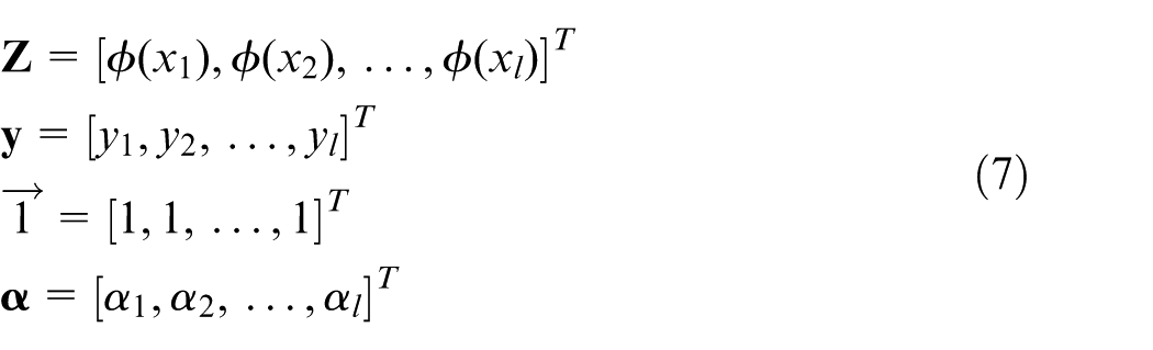
The objective of this article is to develop a tool wear condition-monitoring model for tool wear prediction. Based on the cutting condition parameters during turning operations, LSSVM is used to evaluate the tool wear condition. The rest of this article is organized as follows. LSSVM is adopted to model relationships between tool wear and cutting condition parameters in section “LSSVM-based tool wear prediction model.” In section “Leave-one-out-based LSSVM optimization,” leave-one-out (LOO) technique is used to optimize parameters c and
LSSVM-based tool wear prediction model
SVM is a novel machine-learning tool which is especially useful for classifications and predictions with small sample cases.
16
It is inspired by statistical learning theory leading to a class of algorithms characterized using nonlinear kernels, high generalization ability, and the sparseness of the solution. Unlike the classical neural networks approach, the learning problem formulation of SVM leads to quadratic programming (QP) with linear constraints. However, the size of matrix involved in the QP problem is proportional to the number of training points. Hence, to reduce the complexity of optimization processes, a modified version called LSSVM is proposed by taking equality instead of inequality constraints to obtain a linear set of equations instead of a QP problem in the dual space.17,18 Instead of solving a QP problem as in SVM, LSSVM can obtain the solutions of a set of linear equations. The formulation of LSSVM is introduced as follows. Consider a given training set

where w is the weight vector and b is the bias term. By mapping original input data into a high-dimensional space, the nonlinear separable problem becomes linearly separable in space. Afterward, the following cost function is formulated in the framework of empirical risk minimization as equation (2)
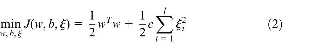
which is subjected to equality constraints

where
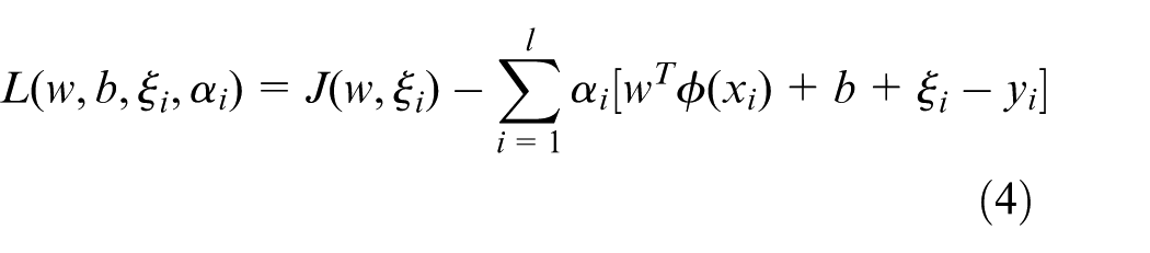
where
According to Karush–Kuhn–Tucker (KKT) rule, the solution of equation (4) can be obtained by partially differentiating with respect to w, b,
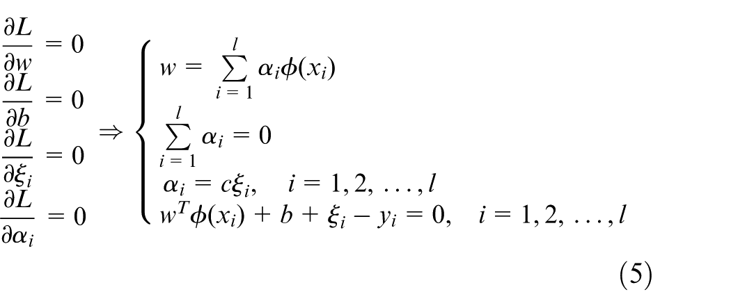
After eliminating w and
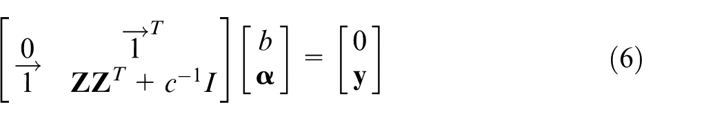
where
The inner-product operation

Optimal
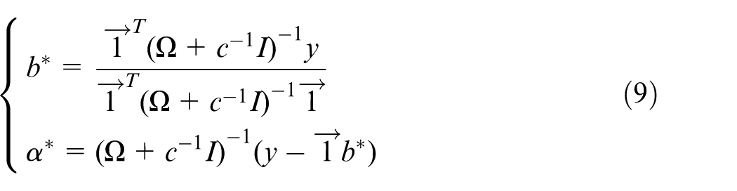
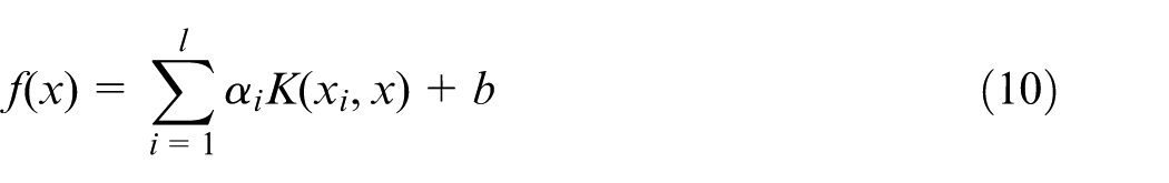
and the result of LSSVM model can be expressed as follows
In comparison with some other feasible kernel functions, the radial basis function (RBF) is a more compact supported kernel, and thus, it is able to reduce computational complexity of the training process and improve generalization performance of LSSVM. As a result, RBF kernel was selected as kernel function as follows
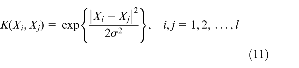
where
Finally, the structure of regression function is shown in Figure 1, the output is a linear combination of intermediate nodes, and each intermediate node corresponds to a support vector. In this article, the input support vectors are tool machining conditions, and the output is tool wear.
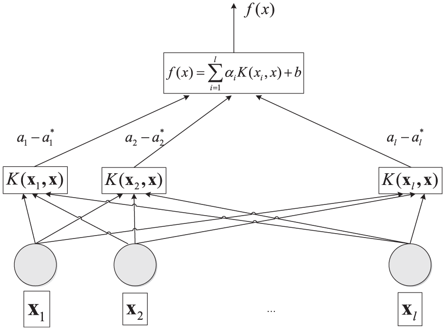
Structure of regression function.
LOO-based LSSVM optimization
In the LSSVM, regularization parameter c and RBF kernel parameter
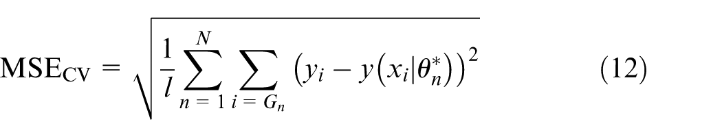
Tuning of regularization parameter c and RBF kernel parameter
where
When N = l,
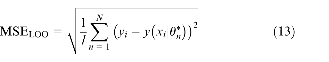
regression function of LSSVM (10) can be rewritten as follows
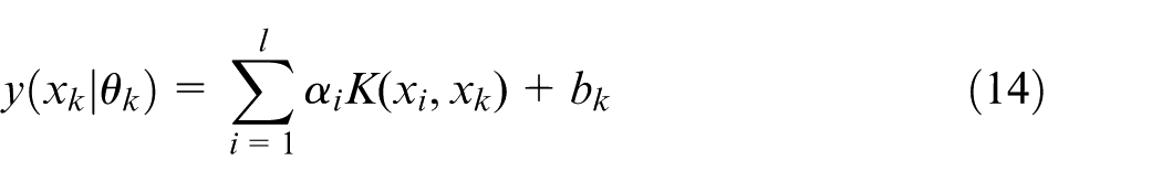
then c can be optimized by calculating the following function
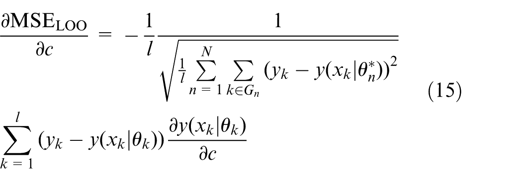
Finally, minimizing equation (15) obtains the optimal c and
Steps to optimize parameters c and
Step 1: Set training points
Step 2: Divide training data set into N segments, where the N − 1 pieces of data are used for training, and the remaining piece of data is used for testing. Get a decision function and the corresponding
Step 3: Use the LOO-LSSVM technique for training and prediction.
NM simplex search method
Although LOO-LSSVM could search the optimum c and
Initialization. For minimization of the n variables unconstrained function, let
Reflection. Determine

where
3. Expansion. If the reflection operation produces a lower vertex, namely

where
If
Exit the algorithm if the stopping criteria are satisfied; if
4. Contraction. It is described as follows: (1) If

where
(2) Exit the algorithm if the stopping criteria are satisfied; if
5. Shrinkage. Following step 4 in which

where
The NM simplex algorithm is simple and demands low analytic properties of the objective function. However, there are two main shortcomings: one is that the choice of initial vertex is very sensitive and the other one is that simplex cannot guarantee the global convergence optimum. 28
NM LOO-based LSSVM-based tool wear prediction model
In order to improve the local search ability of LOO-LSSVM algorithm, NM LOO-based least squares support vector machines (NM-LOO-LSSVM) is proposed. The goal of integrating NM simplex search method and LOO-LSSVM is to combine their advantages and avoid disadvantages. The NM simplex method is a very efficient local search procedure, but the choice of initial points is very sensitive and it is incapable of guaranteeing global optimum. LOO-LSSVM belongs to the class of global search procedure; nonetheless, it lacks local optimum.
NM-LOO-LSSVM algorithm has two stages in each cycle: the first stage is the global search. Based on LOO-LSSVM, global optimum solutions are searched in the solution space of the optimized objective functions, which are as the initial points nearby global optimal solution for the NM simplex method. The second stage is the local search, and further optimization is carried out based on the NM simplex algorithm to find the optimum solution. The whole algorithm process is shown in Figure 2.
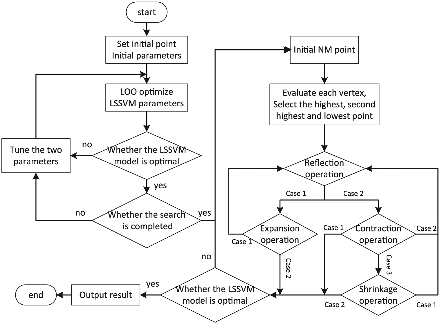
Procedures of NM-LOO-LSSVM model.
Experiments and discussions
Tool wear prediction model
According to prior knowledge of tool wear principles in machining, tool wear changes over machining time, with wear speed is different under different cutting conditions. Under the same cutting condition, rate of wear change is approximately a constant value K
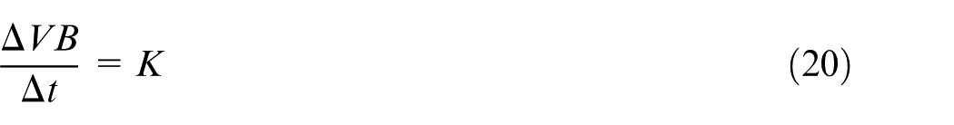
where
Due to the different interactions between the tool and the workpiece, the generating mechanisms of tool wear that include abrasive wear, adhesive wear, and diffusion wear are different. Abrasive wear occurs when the workpiece material is removed from one surface by tool, leaving built-up edge or hard particles of debris between the two surfaces. 29 Abrasive wear is presented under various cutting speeds, but it is the main wear mechanism at low cutting speed. Adhesive wear occurs when minute peaks of the two rough surfaces contact each other and weld or stick together, removing a wear particle. Adhesive wear is more serious under the moderate cutting speed. When cutting temperature is higher than the brittle temperature, tool produces diffusion wear. Experiment showed that with the increase in the cutting speed, carbide cobalt element will decompose into tungsten and carbon diffusing to the steel when cutting temperature is over 800 °C, which makes the tool wear exacerbation. 30
The cutting tools, processing methods, and the macro- and micro-geometry parameters of the tool need to be changed to meet the different processing objects and different precision required constantly in machining, which makes the testing process very complicated. And in one processing step, except changing of the cutting conditions, other factors do not change generally. Therefore, geometric parameters of the tool are fixed in the tool wear condition-monitoring experiment. Different cutting time corresponds to different tool wear conditions. Consequently, cutting time that reflects the entire life cycle of tool is taken into account in this model. Due to complexity of the actual process, the linear relationship does not truly reflect the relationship between tool wear degree and the cutting time interval. Taking different cutting conditions into account, the relationship between tool wear and cutting parameters is constantly changing. Equation (20) generates a highly nonlinear relationship as equation (21)

where a is the cutting depth, f is the feed rate, and v is the spindle speed.
Sample data collection
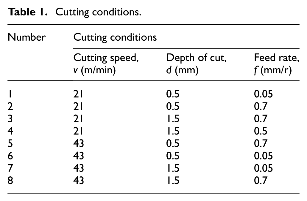
Experiments are performed on CK6143/100 computerized numerical control (CNC) machine with M10 carbide alloy tool and ZMn13 high manganese cast steel, and rake angle γ = 2°, relief angle α = 8°, cutting edge angle kr = 35°. It is desirable that tool wear monitoring model reflects the conditional changes in cutting tools under diverse cutting conditions such as different levels of cutting speed, feed rate, and depth of cut. In experiments, four factors used for the design of experiment were cutting speed, feed rate, depth of cut, and cutting time, which are shown in Table 1.
Cutting conditions.
Tool wear limit is called tool life criterion. In the cutting process, the friction between the tool rake face, flank, and the workpiece will cause high voltage and high temperature on the contact area, where wear occurs. Crater wear occurs on the rake face; flank wear occurs on the tool flank. In many cases, the two occur simultaneously and influence each other. Flank wear has impact on the processing quality, cutting force, and cutting temperature, while the amount of flank wear can be readily observed, measured, and controlled when compared with crater wear. Therefore, the maximum tool flank wear VB is used as tool wear standard in the model of this article.
Experimental methods can be described as follows: the tool is removed from the lathe to observe the flank wear under the microscope after a slot turning. Tool wear is detected every 3 min under each condition to obtain a total of 10 samples. When one slot turning is completed, another slot is ready. Each experiment repeats three times. Every time the tool follows the same cutting path and then detects the amount of wear to avoid the randomness of detection. It should be pointed out that a new cutting tool has been used for each of the eight cutting conditions in each experiment. Experimental conditions, such as cutting fluid performance, the fluid volume, and tool corrected situation, should be strictly controlled for the repeatability of test results in cutting experiments.
In order to avoid differences between each node of sample data, normalization processing was applied to all train and test data as a preprocessing step according to the following function
where x is the uncompressed value,
The whole data set can be further divided into two sub-sets, that is, training data and random test data. Then, the NM-LOO-LSSVM-based tool wear model was trained by training data and two turning parameters c and
Evaluation criteria
To evaluate the performance of NM-LOO-LSSVM model, the following measures are taken:
1. Root MSE
In regression analysis, the term MSE is sometimes used to refer to the unbiased estimate of error variance. 31
2. Coefficient of determination
3. Mean absolute percent error (MAPE)
MAPE measures the method’s accuracy for constructing fitted time series values in statistics, specifically in trend estimation. It usually expresses accuracy as a percentage.
4. Accuracy
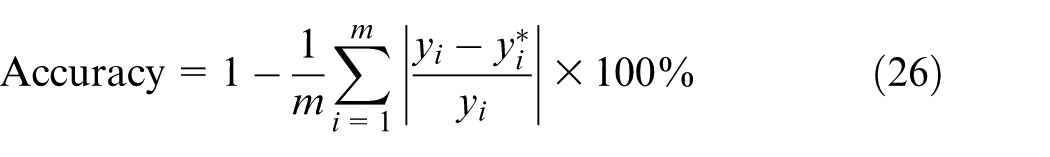
where m is the number of test data,
Sensitivity analysis of NM simplex search parameters
In this section, parameter sensitivity of NM simplex search method will be investigated. The rate of successful minimization is used as the criterion for tuning NM parameters. For the sensitivity investigation, the study is conducted using the original coefficients for NM simplex search method, as shown in Table 2, which also includes ranges of parameters.28,33
Parameter sensitivity ranges.
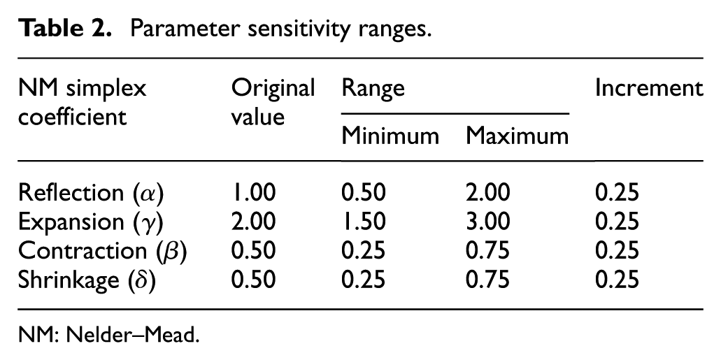
NM: Nelder–Mead.
Each time one of the four parameters is altered according to the ranges given in Table 2, while other three parameters are fixed. For example, in the sensitivity study for reflection coefficient
Figure 3 shows the sensitivity results for the reflection coefficient. As illustrated in the figure, the optimum solutions converge quickly to the minimum value when the reflection coefficient is greater than 0.75, and increment of reflection coefficient does not result in lager oscillation. Additionally, the reflection coefficient setting at 1.5 reaches the best rate of successful minimization. According to equation (16), larger value for the generation of the new vertex
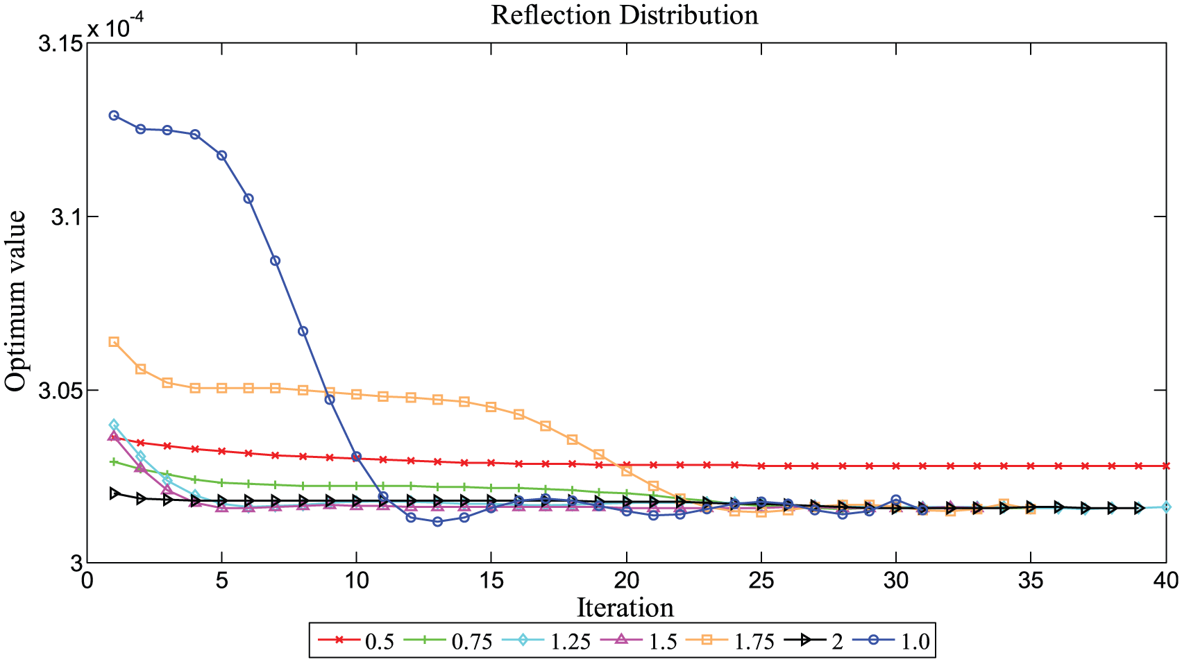
Reflection sensitivity.
Figure 4 shows the sensitivity results for the expansion coefficient. It can be seen that the optimum solutions converge quickly to the minimum value when the expansion coefficient is greater than 1.5, and increment of reflection coefficient does not result in lager oscillation. Also, the expansion coefficient setting at 2.5 achieves the best rate of successful minimization. Equation (17) suggests that the larger value for the generation of the new vertex
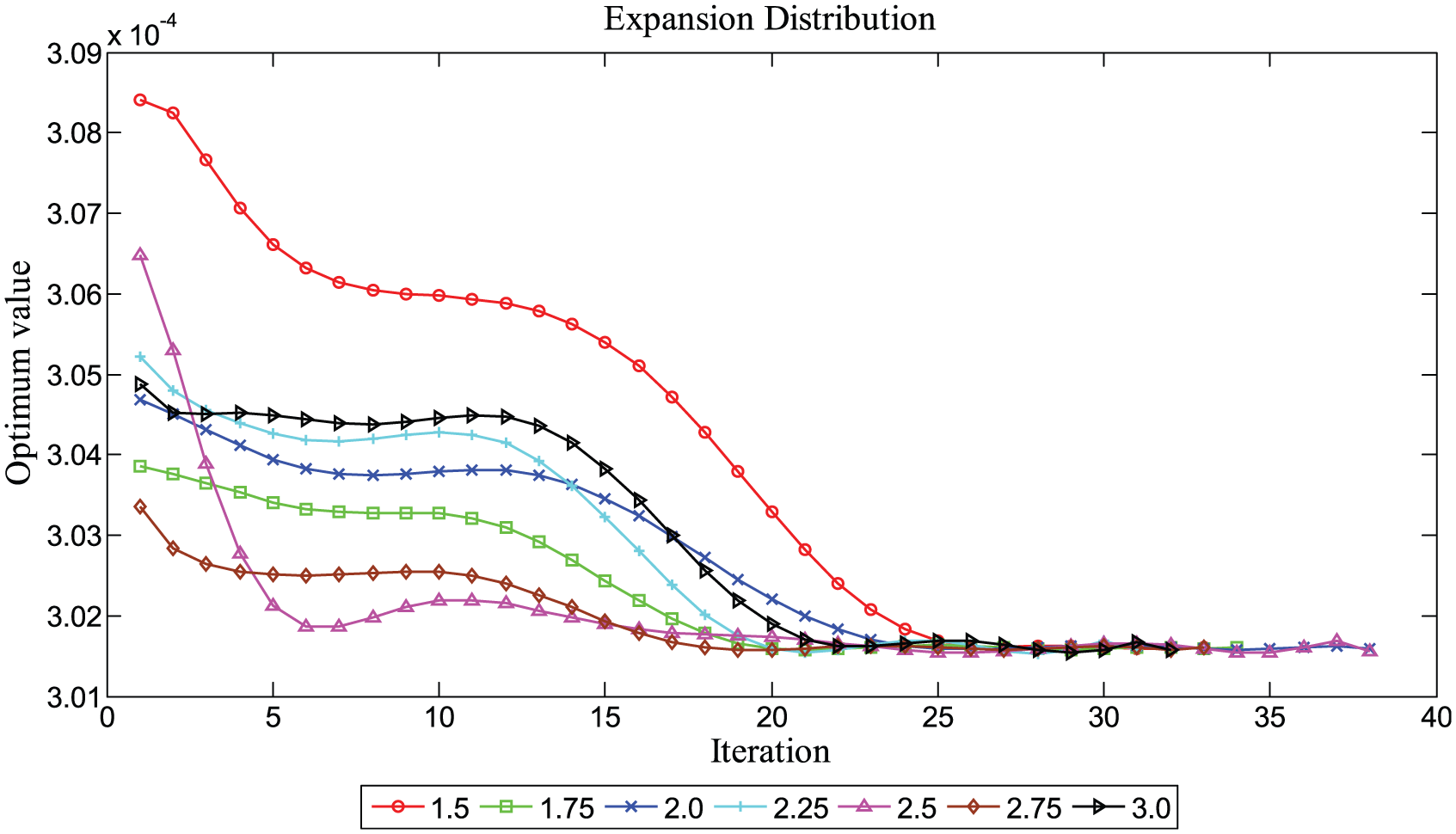
Expansion sensitivity.
Figure 5 shows the sensitivity results for the contraction coefficient. It is observed from Figure 3 that the reflection coefficient setting at 0.75 returns the best rate of successful minimization. Equation (18) suggests that the larger value for the generation of the new vertex
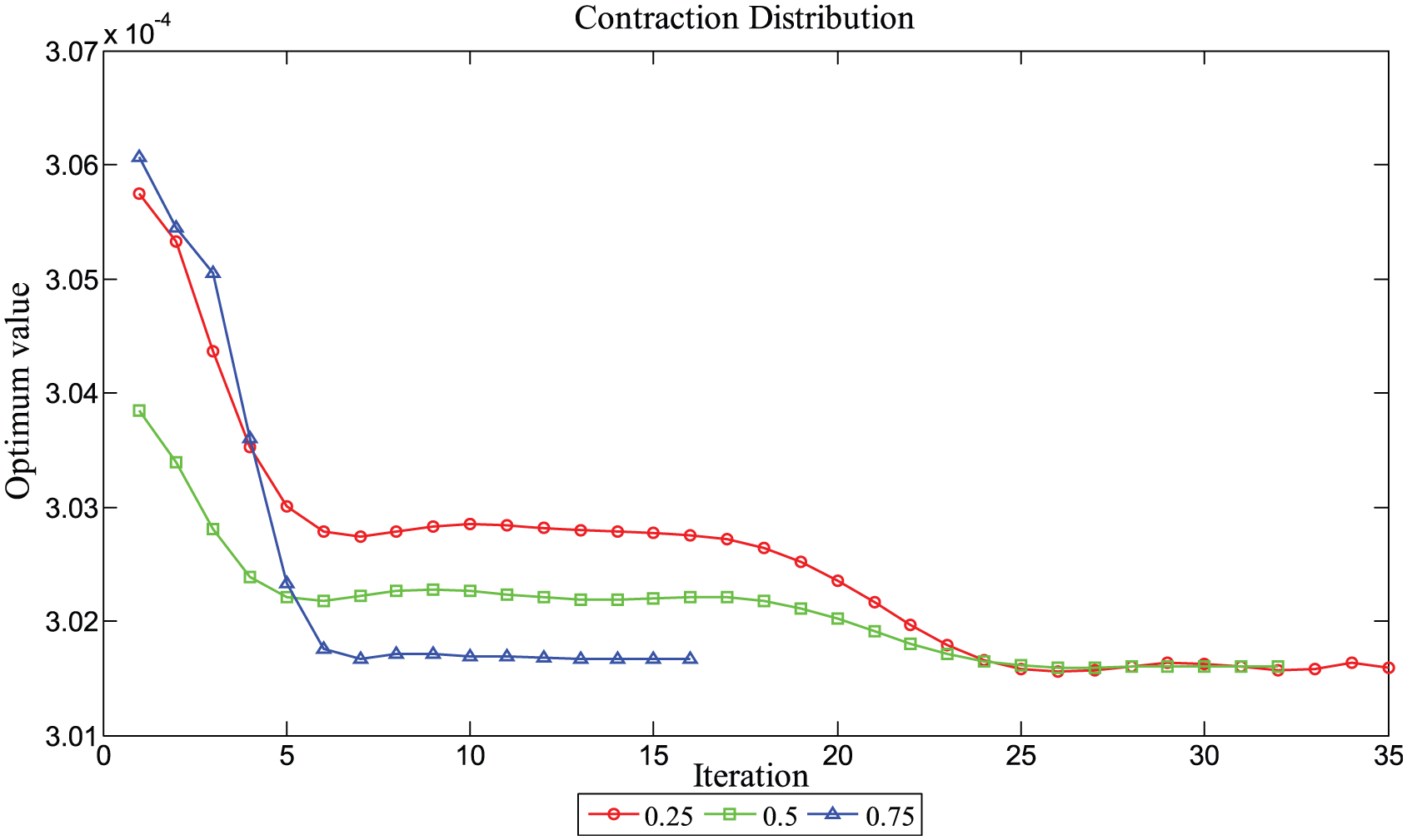
Contraction sensitivity.
Figure 6 shows the sensitivity results for the shrinkage coefficient. It shows that the optimum solutions quickly converge to the minimum value when the shrinkage coefficient is greater than 0.25 for test cases. It is observed from Figure 3 that the shrinkage coefficient setting at 0.5 returns the best rate of successful minimization. Equation (19) suggests that the larger value for the generation of the new vertex
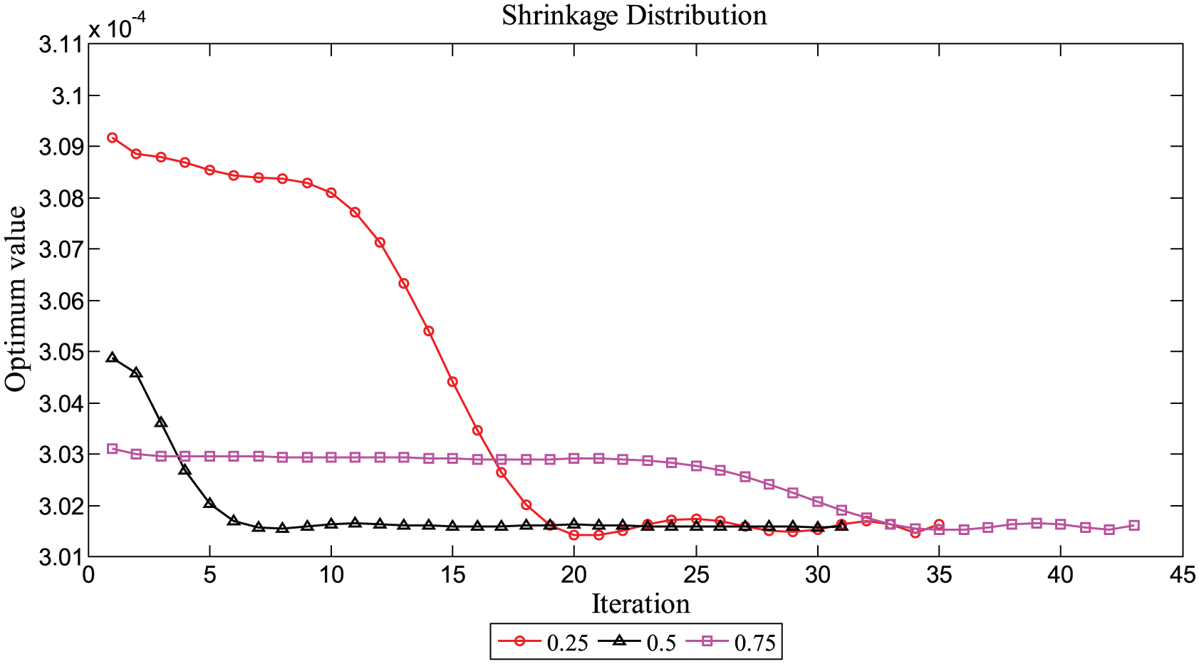
Shrinkage sensitivity.
Reflection coefficient
Best suggested for NM-LOO-LSSVM parameters after sensitivity analysis.
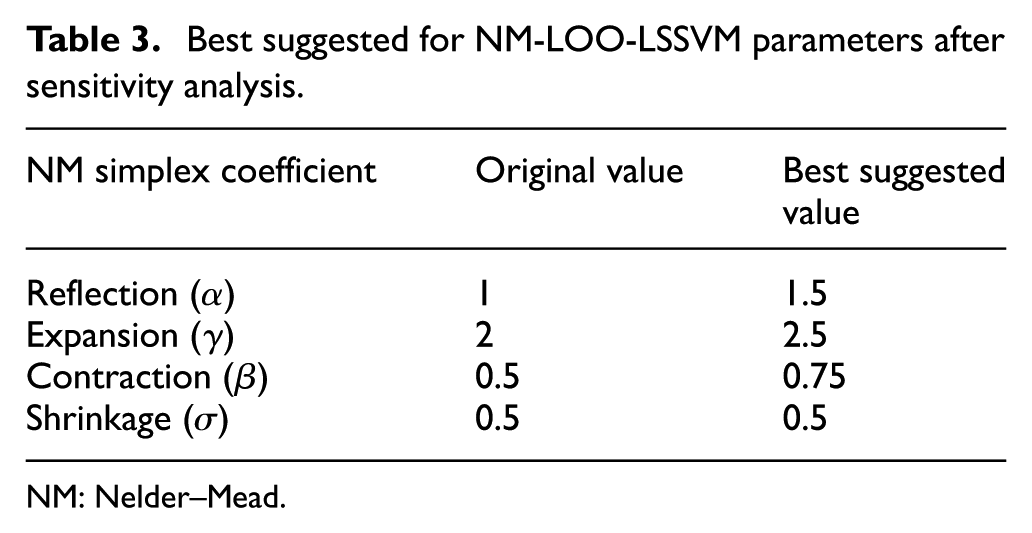
NM: Nelder–Mead.
Experimental results
To validate the effectiveness of the designed algorithm, LSSVM and PSO-LSSVM are used for comparison. The experiments include 10 tests and each has different initial parameters for consideration of data randomness.
The average results of processing are shown in Table 4. It is observed that NM-LOO-LSSVM has the smallest MSE value, largest
Performance of LSSVM, PSO-LSSVM, NM-LOO-LSSVM.
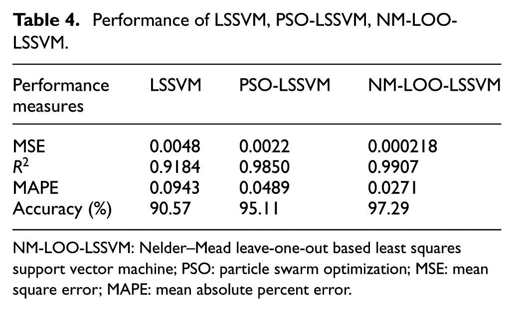
NM-LOO-LSSVM: Nelder–Mead leave-one-out based least squares support vector machine; PSO: particle swarm optimization; MSE: mean square error; MAPE: mean absolute percent error.
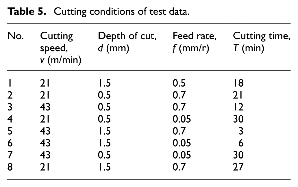
One prediction using LSSVM, PSO-LSSVM, and NM-LOO-LSSVM model, and actual tool wears measured by optical scan microscope are compared as shown in Figure 7. Table 5 lists the cutting conditions of test data. The estimated tool wear, actual tool wear, and fractional error between estimated tool wear and actual tool wear are shown in Table 6. Both the figures and tables demonstrate that NM-LOO-LSSVM and PSO-LSSVM predictions are in accordance with actual tool wears whatever the tool wear level.
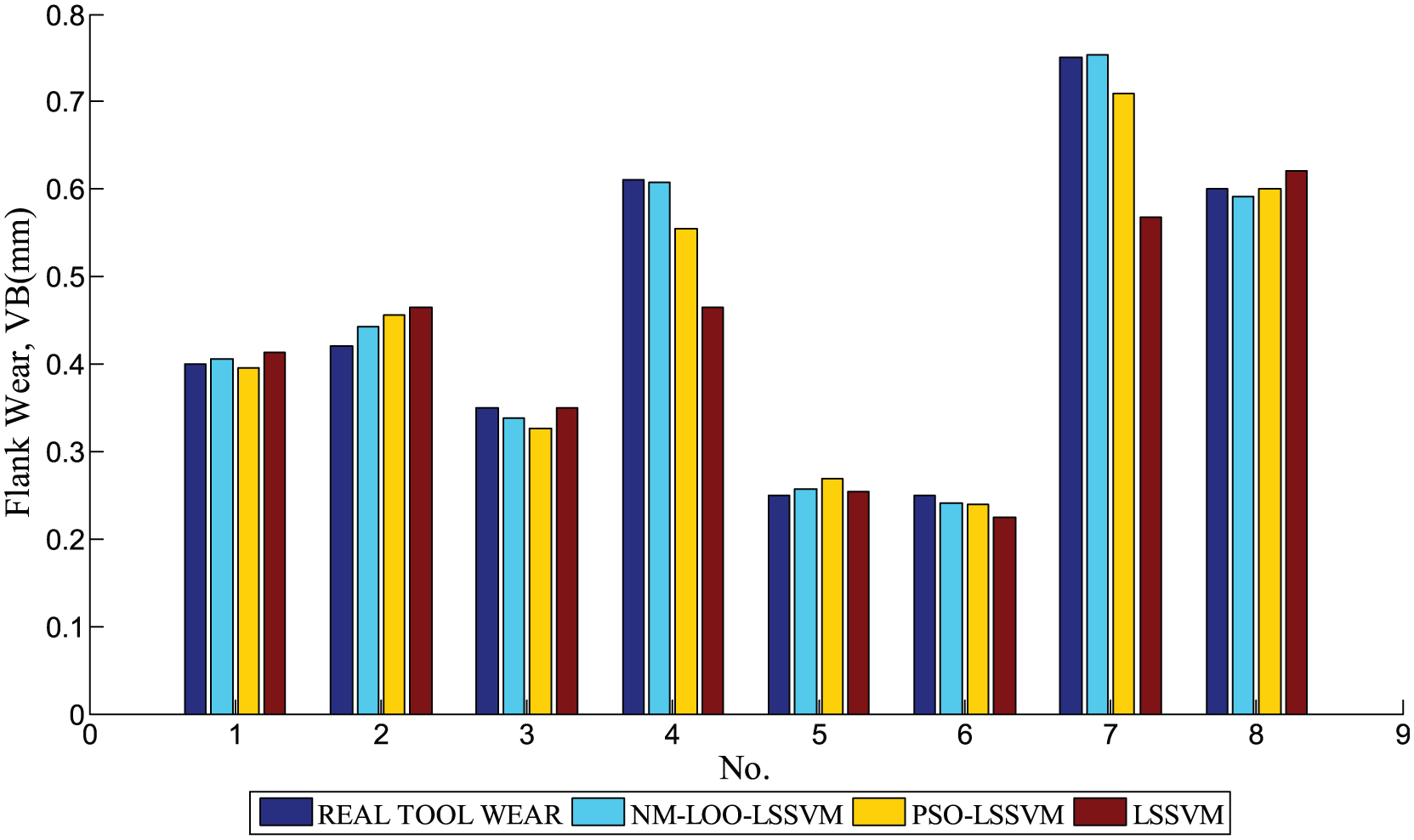
Comparisons between estimated tool wear and actual tool wear.
Cutting conditions of test data.
Fractional error between estimated tool wear and actual tool wear.
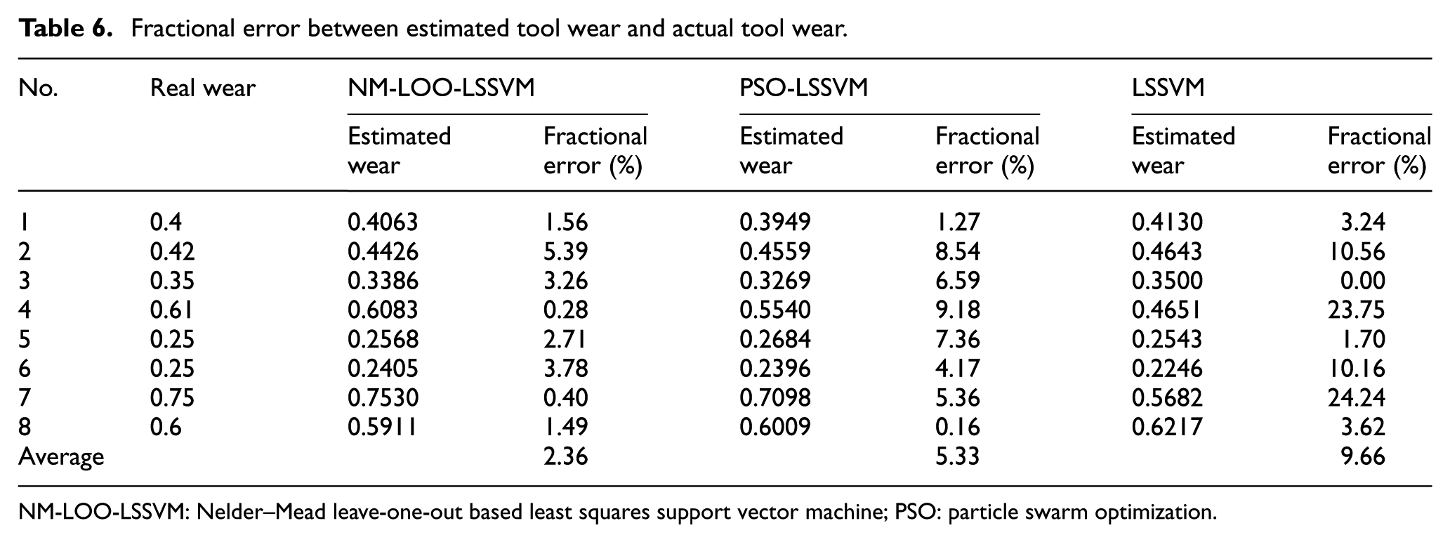
NM-LOO-LSSVM: Nelder–Mead leave-one-out based least squares support vector machine; PSO: particle swarm optimization.
Time consumptions of LSSVM, PSO-LSSVM, and NM-LOO-LSSVM model are compared as shown in Figure 8. As illustrated, NM-LOO-LSSVM model has a running time that is less than 1 s, while PSO-LSSVM exceeds 10 s.
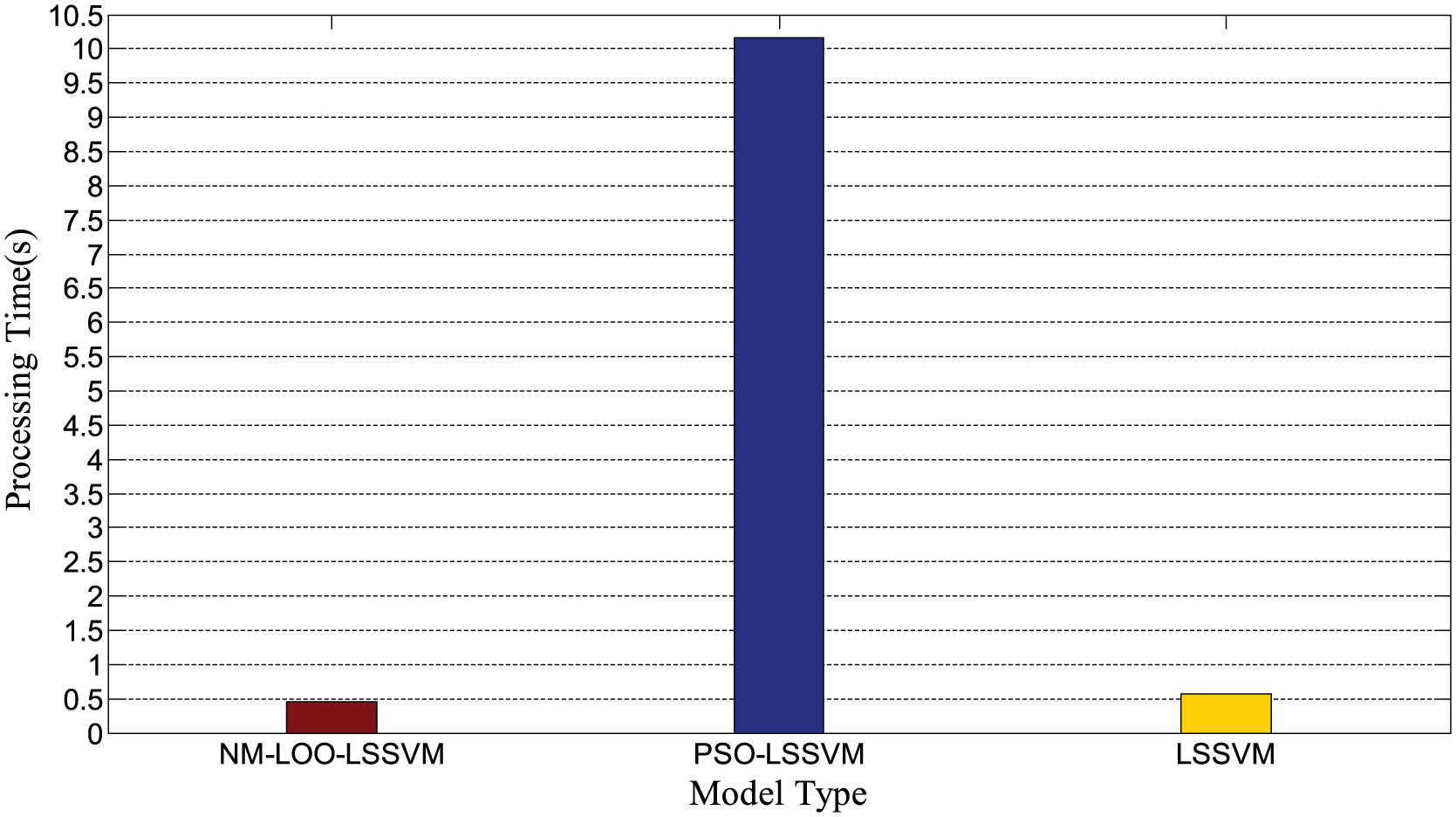
Processing time of LSSVM, PSO-LSSVM, and NM-LOO-LSSVM model.
Results discussion
Table 4 summarizes performances of LSSVM, PSO-LSSVM, and NM-LOO-LSSVM model for tool wear prediction. It is observed from the table that NM-LOO-LSSVM shows the best performance. The MSE value of NM-LOO-LSSVM prediction is smaller than those of the former two, which shows high generalization abilities. The
It is observed from Figure 7 that NM-LOO-LSSVM prediction is most close to the real tool wear on each level intuitively, while prediction of LSSVM is not so good. Table 5 shows the
In Figure 7, the condition #5 (v = 43 m/min; d = 1.5 mm; f = 0.7 mm/r; T = 3 min) results in lower wear as compared with #1 (v = 21 m/min; d = 1.5 mm; f = 0.5 mm/r; T = 18 min). It can be seen that the cutting speed of condition #5 is higher than that of condition #1, while the cutting time of condition #5 is three times less than that of condition #1. As a result, tool wear and cutting time are closely related.
Based on aforementioned elaboration, it can be concluded that accuracies of NM-LOO-LSSVM and PSO-LSSVM are both higher than 95%. However, the PSO-LSSVM model is high in time consumption compared to the NM-LOO-LSSVM model. Figure 8 shows that the convergence rate is also largely improved by the NM-LOO-LSSVM model. Therefore, the established model in this article is the best and fastest method.
The satisfied results of NM-LOO-LSSVM model demonstrate this model’s feasibility for tool wear prediction.
Conclusion
This article establishes a reliable LSSVM model based on NM and LOO techniques focused on the accuracy, generalization, robustness, and convergence rate to predict tool wear. To verify effectiveness of the proposed NM-LOO-LSSVM model, experiments have been conducted. Major contributions of this work are summarized as follows:
A high nonlinear relationship between tool wear and cutting condition parameters is established.
LSSVM techniques have been implemented to predict tool wear based on cutting parameters. LSSVM has good generalization, although sample amount is limited. Furthermore, it also shows excellent global convergence ability due to the use of statistical learning theory.
Parameters sensitivity study is conducted on the NM simplex search method, and relationships between them and their impacts on the optimum solution are investigated. The results show that sensitivity study could reduce NM’s computational cost, thus reaches a faster convergence rate. This study also provides essential insights for designs of other intelligent algorithms.
LOO and NM algorithms are used to tune the LSSVM model to improve the global and local search ability. Analysis results from experiment have shown that NM-LOO-LSSVM can improve the accuracy, generalization, robustness, and convergence of the regression. This is critical since NM-LOO-LSSVM can reduce LSSVM’s failure risks of falling into a global minimum value.
This article not only has studied the tool wear prediction, but also has established a fast and accurate predictive model. This study has done a lot of cutting experiments under certain cutting conditions. Therefore, conclusions of the experiment analysis have some inevitable limitations. Due to the limited actual conditions, the tool wear condition-monitoring model of this article has not yet been used for online real-time monitoring in practical applications. Future research in the real production environment is needed to further validate the study. Meanwhile, the predictive ability of the model depends on the existing knowledge base. When a new processing environment appears, the prediction does not match the actual situation well, which leads to misjudgments. Therefore, this article offers guidance to online real-time tool wear monitoring and product applications.
In the conclusion, this article studies tool wear prediction under different cutting conditions and aims at dealing with the disadvantage of single cutting condition. And mapping relationships between tool wear and four cutting conditions are explored, which indicates that more tool cutting conditions can be explored. Experimental results validate the effectiveness of NM-LOO-LSSVM model since the estimation error is acceptable. This model provides an effective, reliable solution for optimization of tool machining condition, which can be used for real industrial applications with its high accuracy and rapid convergence. According to the desired tool life, tool cutting parameters can be adjusted to make estimated tool life by selecting tool and materials. Therefore, the production efficiency could be efficiently improved.
Footnotes
Acknowledgements
The authors would like to express their thanks to related financial supports. The authors express their gratitude to Yang Cao for the language help.
Declaration of Conflicting Interests
The author(s) declared no potential conflicts of interest with respect to the research, authorship, and/or publication of this article.
Funding
The author(s) disclosed receipt of the following financial support for the research, authorship, and/or publication of this article: This study was supported by the National Science and Technology Support Plan Subsidization Project (Grant No. 2014BAF08B02), the National Science and Technology Major Project (Grant No. 2012ZX04011-031), National Outstanding Youth Science Foundation (Grant No. 50925518), and the Youth Science Foundation of National Natural Science Foundation (Grant No. 51005260).