Sage Journals: Discover world-class research

Abstract

The specific energy consumption of machine tools and surface roughness are important indicators for evaluating energy consumption and surface quality in processing. Accurate prediction of them is the basis for realizing processing optimization. Although tool wear is inevitable, the effect of tool wear was seldom considered in the previous prediction models for specific energy consumption of machine tools and surface roughness. In this paper, the prediction models for specific energy consumption of machine tools and surface roughness considering tool wear evolution were developed. The cutting depth, feed rate, spindle speed, and tool flank wear were featured as input variables, and the orthogonal experimental results were used as training points to establish the prediction models based on support vector regression (SVR) algorithm. The proposed models were verified with wet turning AISI 1045 steel experiments. The experimental results indicated that the improved models based on cutting parameters and tool wear have higher prediction accuracy than the prediction models only considering cutting parameters. As such, the proposed models can be significant supplements to the existing specific energy consumption of machine tools and surface roughness modeling, and may provide useful guides on the formulation of cutting parameters.

Keywords

Prediction model specific energy consumption of machine tools surface roughness cutting parameters tool wear support vector regression

Introduction

As the basic devices in machining system, machine tools have large quantity with high energy consumption. However, their energy efficiency is very low, with an average of less than 30%.¹ In addition, the greenhouse gas emissions caused by the use of machine tools cannot be ignored.² Gutowski³ pointed out that the CO₂ emissions of a computer numerical control (CNC) machine tool with spindle power in 22 kW operating 1 year is equivalent to the emissions of 61 sport utility vehicles (SUVs). Consequently, the urgent task of manufacturing industry is how to reduce energy consumption and carbon emission to achieve sustainable development on the premise of ensuring the processing quality.^4,5

Reducing the energy consumption in machining can significantly improve the environmental performance of manufacturing industry.⁶ In this regard, Rao⁷ presented some schemes for reducing the energy consumed in grinding, which paves the way for improved energy-efficient manufacturing processes. The basic energy-saving approach is to monitor and evaluate energy consumption of machine tools.⁸ Therefore, many scholars have investigated energy consumption characteristics of machine tools and made valuable contributions toward reliable and accurate energy consumption and power demand modeling. For example, Draganescu et al.⁹ and Zhang et al.¹⁰ presented energy consumption models of machine tools from the viewpoint of cutting force, respectively. Gutowski et al.¹¹ proposed a total power model of machine tools as a linear function of the material removal rate (MRR). Based on the relationship between energy consumption of machine tools and MRR, Kara and Li obtained an energy consumption prediction model suitable for turning and milling.^12,13 It is worth noticing that MRR is the only independent variable in aforementioned models. However, the cutting experiments indicate that the energy consumption of machine tools under the same MRR and different cutting parameters is not always equal. In this regard, Zhou et al.¹⁴ compared the prediction accuracy between the model based on MRR and the model based on cutting parameters. Their conclusion is that the latter model with cutting parameters as independent variables obtains higher prediction accuracy. Li et al.¹⁵ developed a model as a function of MRR and spindle speed, which can realize the prediction of energy consumption in face milling. Besides, He et al.¹⁶ presented a method to estimate the energy consumption of machine tools, which can be used to optimize the numerical control (NC) codes to improve energy efficiency. Most of the preceding studies characterize the relationship between the energy consumption of machine tools and cutting parameters based on empirical modeling. However, these traditional energy consumption models fail to take the effect of tool wear into consideration.

Actually, the cutting experiments with the same workpiece material and cutting parameters show that the cutting power is different as the tool wears gradually. Axinte and Gindy assessed the sensitivity of spindle power for tool wear in turning, milling, and drilling.¹⁷ For the purpose of tool condition monitoring, Cuppini et al.¹⁸ analyzed the relationship between cutting power of machine tools and tool wear. In addition, Li et al.¹⁹ established a regression model of cutting power based on cutting parameters and tool wear using the response surface method (RSM) for tool change decision. Although these studies are not intended to estimate the energy consumption of machine tools, they indicate that tool wear can affect the energy consumption of machine tools in machining.

Recently, several scholars have taken tool wear into consideration and made further research on the energy consumption of machine tools. For instance, Yoon et al.²⁰ investigated the energy consumption of machine tools under slight, medium, and severe tool wear conditions. Their experimental results showed that the increase of tool wear leads to more energy consumption in machining. Additionally, Liu et al.²¹ explored the effect of MRR and tool wear on energy consumption at the machine tool, spindle, and process levels in hard milling AISI H13. Their conclusion is that the tool wear has the significant influence on the specific energy consumption of the process level. However, these models were established with few conditions of tool wear, which cannot fully reflect the effect of tool wear evolution on energy consumption of machine tools. In this regard, Zhao et al.²² developed an empirical model to predict tool tip cutting specific energy consumption based on cutting parameters and tool flank wear in milling. In fact, the condition of tool wear changes constantly because of the friction between the tool and the workpiece in cutting stage.

Although sustainable manufacturing requires manufacturers to save energy and reduce emissions as much as possible, the premise is to guarantee the processing quality. The workpiece surface quality usually has a great influence on mechanical performance of machined parts. In general, the improvement of energy efficiency in machining will lead to the deterioration of surface roughness. In order to solve this problem, techniques such as hybrid decision analysis, Taguchi method, and gray correlation analysis are used for multi-objective optimization of cutting parameters.^23–25 However, accurate prediction of surface roughness is the basis for processing optimization. Thus, as an important indicator for evaluating the processing quality, surface roughness also needs to be accurately predicted. In theory, surface roughness is closely related to cutting conditions (e.g. cutting parameters, cutting fluid, tool geometric parameters, and tool-workpieces properties). Various studies have made important contributions to the prediction and control of surface roughness. For instance, Arapoğlu et al.²⁶ and Imani et al.²⁷ established surface roughness prediction models based on artificial neural networks (ANN) in turning and milling, respectively. Debnath et al.²⁸ studied the influence of various cutting fluid levels and cutting parameters on surface roughness in turning. Patel and Gandhi built a mathematical model for surface roughness in turning AISI D2, which is exponentially related to feed rate, cutting speed, and tool nose radius.²⁹ In addition, RSM is often used as a powerful design-of-experiment (DoE) technique when dealing with surface roughness. Using RSM, Kosaraju and Anne³⁰ proposed a model for surface roughness based on cutting speed, feed rate, cutting depth, and back rake angle to select optimal cutting parameters in turning Ti-6Al-4V. Similarly, Parida and Maity³¹ developed a model for surface roughness in hot turning Monel 400, which is based on cutting speed, feed rate, cutting depth, and workpiece temperature. However, these models were based on a common assumption that the condition of tool wear remains unchanged in machining, without considering the effect of tool wear evolution on surface roughness. In truth, worn tools harmfully affect surface roughness and the performance of machined parts.

In sum, the energy consumption of machine tools and surface roughness modeling with tool wear evolution have not been solved to a satisfactory degree, and further effort is needed for a more comprehensive solution. The support vector regression (SVR) is one of machine learning (ML) algorithms,³² which can effectively solve the problem of nonlinear regression. Compared with ANN and random forest (RF), SVR has better prediction accuracy and shorter running time when the amount of training set is small.³³ Accordingly, it has been widely used in the field of machining, such as predicting surface roughness and tool wear.^34,35

The objectives of this paper are to: (1) consider the effect of tool wear evolution on energy consumption of machine tools and surface roughness; (2) introduce SVR algorithm to develop the prediction models for specific energy consumption of machine tools and surface roughness based on cutting parameters and tool wear; and (3) verify the proposed models with wet turning experiments of AISI 1045 steel.

Experimental and SVR modeling details

Experimental design

CNC turning operations

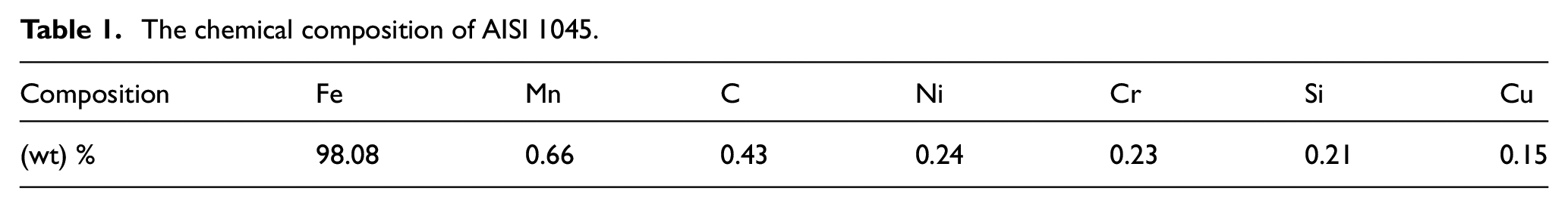
As a kind of high-quality carbon structural steel, AISI 1045 steel is widely used in the production of bolts, shafts, and guide pins. It was selected as the workpiece material, and the chemical composition of AISI 1045 is shown in Table 1. The diameter of workpieces was 55 mm, with processing length 120 mm. Wet turning of AISI 1045 steel was performed at a CNC lathe (Yishui CKJ6163, Figure 1) with carbide cutting inserts (SKYWALKER CNMG120408-PG SC4025). The workpiece surface was turned prior to any experiments in order to remove surface defects.

Table 1.

The chemical composition of AISI 1045.

Composition	Fe	Mn	C	Ni	Cr	Si	Cu
(wt) %	98.08	0.66	0.43	0.24	0.23	0.21	0.15

Figure 1.

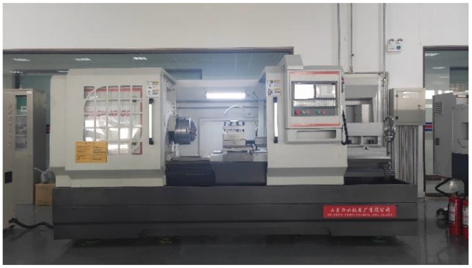
Yishui CKJ6163 lathe.

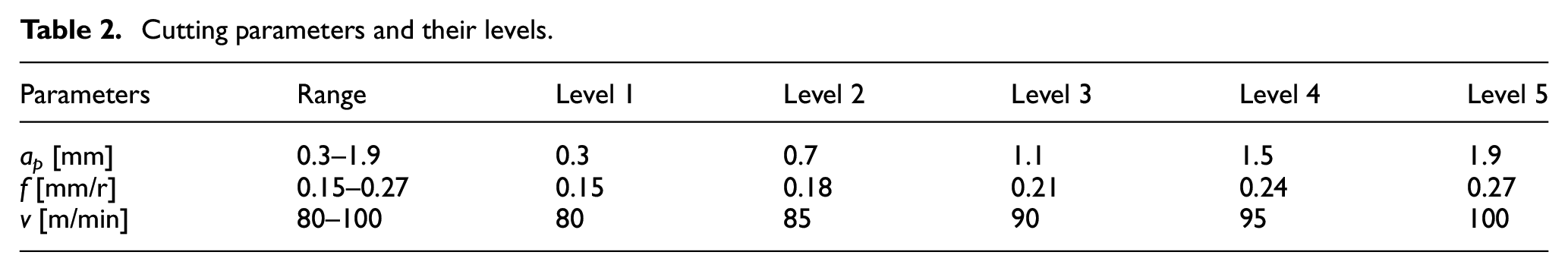
The ranges of cutting parameters (cutting depth a_p, feed rate f, and cutting speed v) were customized within the ranges recommended by the cutting insert manufacturer. In order to reduce the cost of tests and improve the efficiency, the L₂₅ (5³) orthogonal experiments with 25 sets of three factors and five levels were designed with Taguchi method. Table 2 shows cutting parameters and their levels. The spindle speed n was used in CNC programming, it can be calculated by equation (1).

n = \frac{1000 v}{π d}

(1)

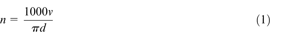
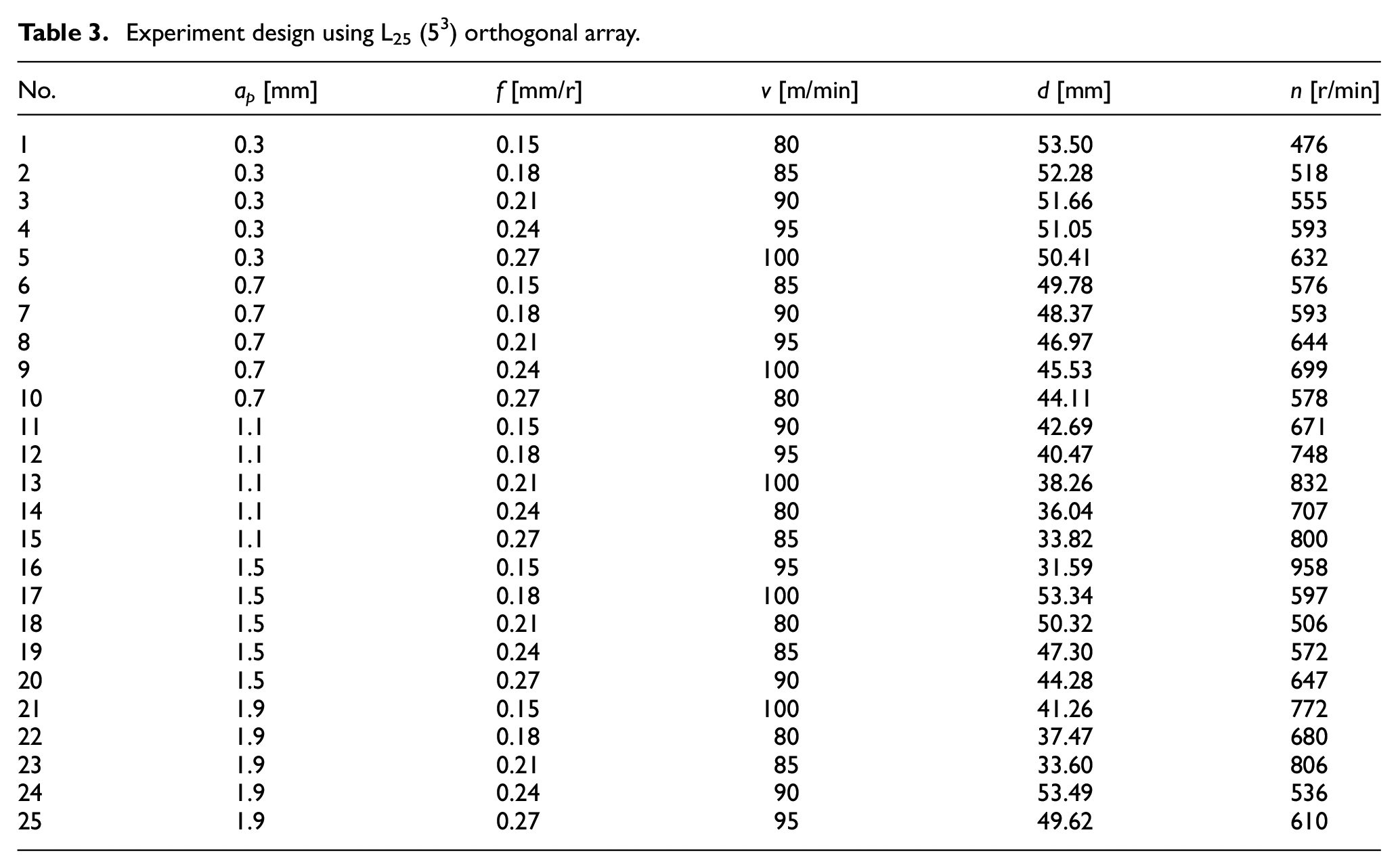
where n is spindle speed in r/min; v is cutting speed in m/min; and d is workpiece diameter in mm. Experimental combinations of the cutting parameters are presented in Table 3.

Table 2.

Cutting parameters and their levels.

Parameters	Range	Level 1	Level 2	Level 3	Level 4	Level 5
a_p [mm]	0.3–1.9	0.3	0.7	1.1	1.5	1.9
f [mm/r]	0.15–0.27	0.15	0.18	0.21	0.24	0.27
v [m/min]	80–100	80	85	90	95	100

Table 3.

Experiment design using L₂₅ (5³) orthogonal array.

No.	a_p [mm]	f [mm/r]	v [m/min]	d [mm]	n [r/min]
1	0.3	0.15	80	53.50	476
2	0.3	0.18	85	52.28	518
3	0.3	0.21	90	51.66	555
4	0.3	0.24	95	51.05	593
5	0.3	0.27	100	50.41	632
6	0.7	0.15	85	49.78	576
7	0.7	0.18	90	48.37	593
8	0.7	0.21	95	46.97	644
9	0.7	0.24	100	45.53	699
10	0.7	0.27	80	44.11	578
11	1.1	0.15	90	42.69	671
12	1.1	0.18	95	40.47	748
13	1.1	0.21	100	38.26	832
14	1.1	0.24	80	36.04	707
15	1.1	0.27	85	33.82	800
16	1.5	0.15	95	31.59	958
17	1.5	0.18	100	53.34	597
18	1.5	0.21	80	50.32	506
19	1.5	0.24	85	47.30	572
20	1.5	0.27	90	44.28	647
21	1.9	0.15	100	41.26	772
22	1.9	0.18	80	37.47	680
23	1.9	0.21	85	33.60	806
24	1.9	0.24	90	53.49	536
25	1.9	0.27	95	49.62	610

Tool wear and surface roughness measurement

Tool flank wear is always considered to be the main subject of tool wear and the standard of tool bluntness.³⁶ Therefore, the flank wear of the cutting inserts was measured in this research. The tool wear measurement system (as shown in Figure 2) consisted of a microscope (ZEISS Axio Lab.A1 Mat) and its image analysis software. The flank wear of cutting inserts was measured twice before and after each turning, and the average value was taken as the tool wear VB. In addition, the maximum allowable tool flank wear has been set to be VB_max = 0.27 mm, which means that the cutting inserts will be replaced if the wear length reaches 0.27 mm. Since tool wear measurement required cutting inserts to be removed from the tool holder, the tool placement error was eliminated by re-setting the tool before the next experiment.

Figure 2.

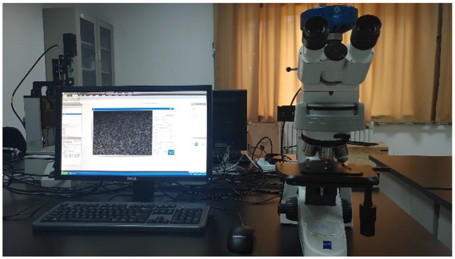
Tool wear measurement system.

The workpiece surface roughness was measured (as shown in Figure 3) with the surface roughness tester RTP120. The surface roughness tester was placed on the sliding table after each turning. Measurements from three different locations were carried out, and the average value was taken as the surface roughness Ra in each experiment.

Figure 3.

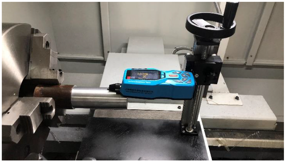
Surface roughness measurements.

Machine tool power measurement and specific energy consumption calculation

The complete CNC lathe working process includes start-up, standby, spindle start, no-load operation, cutting stage, no-load operation, spindle stop, standby, and shutdown. In general, cutting stage is the most energy-consuming working process. In this stage, the energy-consuming components of machine tools include machine control unit (MCU), spindle motor, feed-axis motors, cooling pump motor, and lighting device. Therefore, the energy consumption of machine tools in cutting stage is the focus of this study.

The cutting power of machine tools was measured with a power analyzer (Yokogawa WT500) and shunts. The voltage signals and current signals of lathe were connected to the power analyzer, and a personal computer (PC) was connected to the power analyzer for recording and processing power signals. Figure 4 shows the hardware configuration used for the power measurement system.

Figure 4.

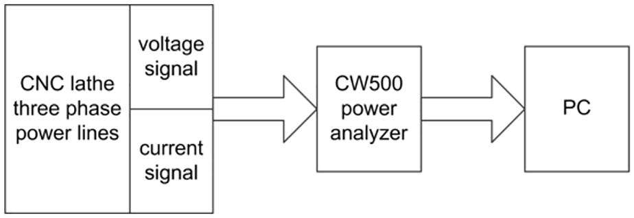
Hardware configuration for the power measurement system.

The specific energy consumption was employed to evaluate the energy efficiency of machine tools, which is defined as the energy consumption to remove a unit volume of material.¹³ Once the specific energy of machine tools is known, the total energy consumption of machine tools can be accurately predicted. The specific energy consumption of machine tools can be calculated by equation (2).

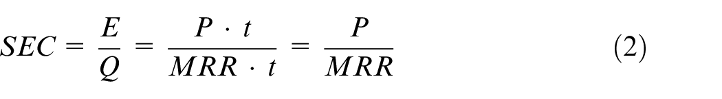
SEC = \frac{E}{Q} = \frac{P \cdot t}{MRR \cdot t} = \frac{P}{MRR}

(2)

where SEC is the specific energy consumption of machine tools in J/mm³; E is the energy consumption of machine tools in J; Q is the total material removal volume in mm³; P is the total power of machine tools in cutting stage in W; MRR is material removal rate in mm³/s; and t is the cutting time in s. Moreover, the material removal rate in turning can be obtained by equation (3).

MRR = \frac{π [{(\frac{d}{2})}^{2} - {(\frac{d}{2} - a_{p})}^{2}] nf}{60}

(3)

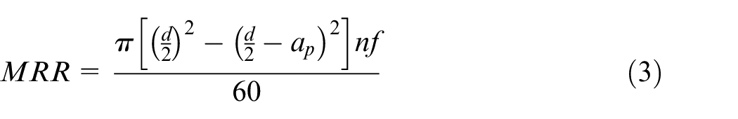
where d is workpiece diameter in mm; n is spindle speed in r/min; f is feed rate in mm/r; and a_p is cutting depth in mm.

SVR modeling

In this section, SVR algorithm was introduced to establish the prediction models for SEC and Ra. The essence of SVR modeling is to find an optimal classification surface, so that the distance error from all training points to the classification surface is minimized.³² For comparative analysis, two kinds of prediction models were established using the 25 sets of orthogonal experiment data. The first kind of prediction models (SEC₁ and Ra₁) was based on cutting parameters, the other proposed (SEC₂ and Ra₂) was based on cutting parameters and tool wear.

Running of SVR

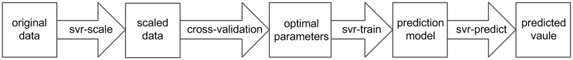
The flowchart of SVR modeling is shown in Figure 5, including the following five steps.

Step 1: transform the experiment data to the format of an SVR package.

Step 2: conduct scaling on the original experiment data. The input variables are scaled to [−1, 1] to eliminate the dimension differences and improve the training efficiency of models.

Step 3: find the optimal parameters. The radial basis function (RBF, see equation (4)) is selected as the kernel function, and the key parameters of SVR algorithm, i.e., constant coefficient C, kernel function parameter g, and loss function parameter p are searched by cross-validation.

K (x, y) = \exp (- g ‖ x - y ‖^{2})

(4)

Step 4: use the optimal parameters to train the whole training set to obtain the prediction model.

Step 5: test.

Figure 5.

The flowchart of SVR modeling.

Prediction models based on cutting parameters

According to metal cutting theory, the cutting power and surface roughness are closely related to cutting parameters. Hence, the prediction models (SEC₁ and Ra₁) based on cutting parameters were presented. There were three inputs and one output in SEC₁ and Ra₁. Specifically, a_p, f, and n were featured as input variables, with SEC and Ra were taken as target values, respectively, as shown in Figure 6.

Figure 6.

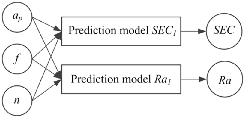
Prediction models based on cutting parameters.

Prediction models based on cutting parameters and tool wear

Using the same workpiece and cutting parameters, the cutting power and surface roughness will increase as the cutting insert gradually wears. Therefore, specific energy consumption of machine tools and surface roughness are not only related to cutting parameters, but also tool wear condition. The prediction models (SEC₂ and Ra₂) based on cutting parameters and tool wear were developed. There were four inputs and one output in SEC₂ and Ra₂. To be specific, a_p, f, n, and VB were featured as input variables, with SEC and Ra were taken as target values, respectively, as shown in Figure 7.

Figure 7.

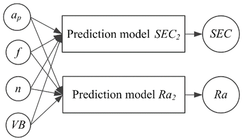
Prediction models based on cutting parameters and tool wear.

Results and discussion

Experimental results

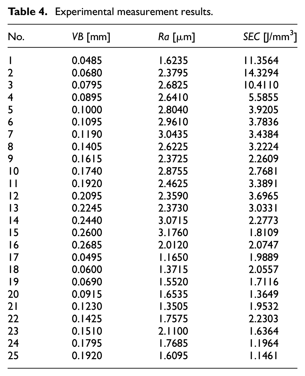
About 25 sets of experimental measurement and calculation results (VB, Ra, and SEC) are presented in Table 4.

Table 4.

Experimental measurement results.

No.	VB [mm]	Ra [µm]	SEC [J/mm³]
1	0.0485	1.6235	11.3564
2	0.0680	2.3795	14.3294
3	0.0795	2.6825	10.4110
4	0.0895	2.6410	5.5855
5	0.1000	2.8040	3.9205
6	0.1095	2.9610	3.7836
7	0.1190	3.0435	3.4384
8	0.1405	2.6225	3.2224
9	0.1615	2.3725	2.2609
10	0.1740	2.8755	2.7681
11	0.1920	2.4625	3.3891
12	0.2095	2.3590	3.6965
13	0.2245	2.3730	3.0331
14	0.2440	3.0715	2.2773
15	0.2600	3.1760	1.8109
16	0.2685	2.0120	2.0747
17	0.0495	1.1650	1.9889
18	0.0600	1.3715	2.0557
19	0.0690	1.5520	1.7116
20	0.0915	1.6535	1.3649
21	0.1230	1.3505	1.9532
22	0.1425	1.7575	2.2303
23	0.1510	2.1100	1.6364
24	0.1795	1.7685	1.1964
25	0.1920	1.6095	1.1461

Numerical results

Training results of SVR models

With the help of LIBSVM 3.23 toolbox in windows cmd.exe (Appendix A),³⁷ both kinds of prediction models were established. The selection of parameters and training results of SVR models are as follows.

For SEC₁, the optimal parameters found by cross-validation are C = 64, g = 0.5, and p = 0.0625. Additionally, the mean square error MSE of the model is 0.177892, and the determination coefficient R² is 0.985971. The comparison of measured-predicted values from SEC₁ is depicted in Figure 8. With regard to Ra₁, the optimal parameters found by cross-validation are C = 4, g = 0.25, and p = 0.5. The MSE of the model is 0.125451, and R² is 0.660473. The comparison of measured-predicted values from Ra₁ is depicted in Figure 9.

Figure 8.

Comparison of measured-predicted values from SEC₁.

Figure 9.

Comparison of measured-predicted values from Ra₁.

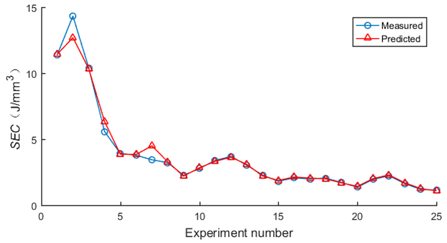
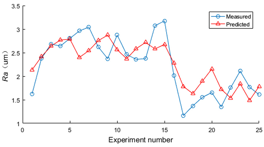
For SEC₂, the optimal parameters found by cross-validation are C = 16, g = 2.2974, and p = 0.01. The MSE of the model is 1.00584e⁻⁴, and R² is 0.99995. Figure 10 shows the comparison of measured-predicted values from SEC₂. With regard to Ra₂, the optimal parameters found by cross-validation are C = 32, g = 0.5, and p = 0.0078125. The MSE of the model is 6.0567e⁻⁵, and R² is 0.9998450. Figure 11 shows the comparison of measured-predicted values from Ra₂.

Figure 10.

Comparison of measured-predicted values from SEC₂.

Figure 11.

Comparison of measured-predicted values from Ra₂.

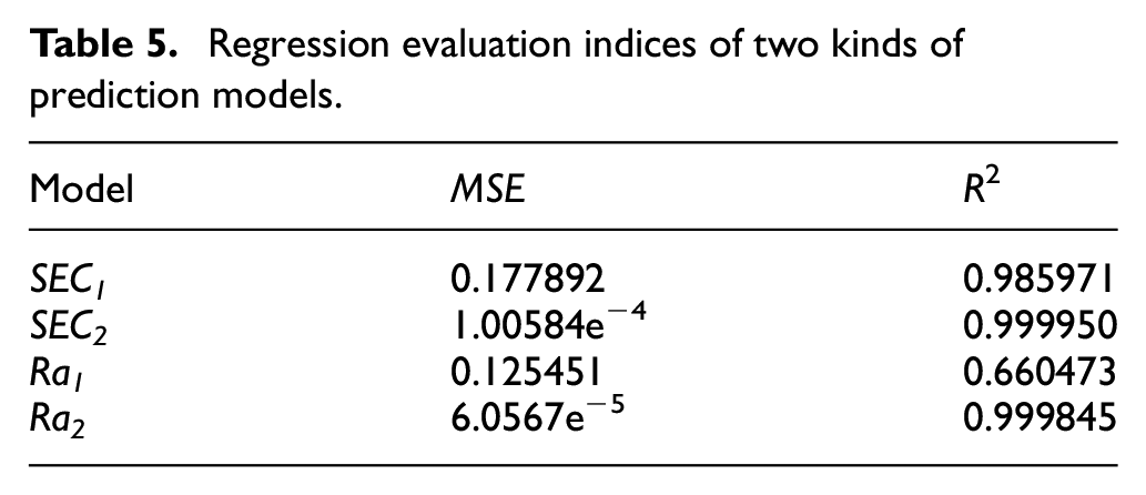
The mean square error MSE and the determination coefficient R² are widely used to evaluate regression effect in SVR modeling. The smaller the value of MSE and the larger the value of R², the better the model fitting effect and the higher the prediction accuracy. The regression evaluation indices of two kinds of prediction models are presented in Table 5. From the training results, the MSE of SEC₂ and Ra₂ are smaller than SEC₁ and Ra₁, and the R² of SEC₂ and Ra₂ are larger than SEC₁ and Ra₁, which indicates that SEC₂ and Ra₂ achieve higher fitting accuracy.

Table 5.

Regression evaluation indices of two kinds of prediction models.

Model	MSE	R ²
SEC₁	0.177892	0.985971
SEC₂	1.00584e⁻⁴	0.999950
Ra₁	0.125451	0.660473
Ra₂	6.0567e⁻⁵	0.999845

Test results of SVR models

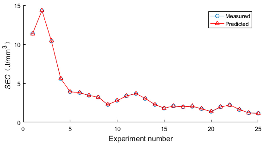
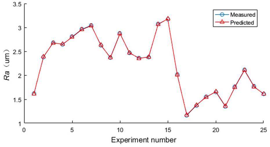
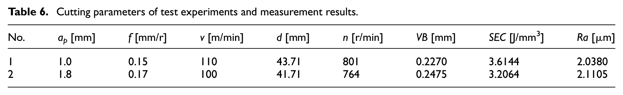
New combinations of cutting parameters were designed to test the above two kinds of prediction models. The experimental cutting parameters and measurement results are presented in Table 6, and the test results when adopting two kinds of models are compared in Figures 12 and 13.

Table 6.

Cutting parameters of test experiments and measurement results.

No.	a_p [mm]	f [mm/r]	v [m/min]	d [mm]	n [r/min]	VB [mm]	SEC [J/mm³]	Ra [μm]
1	1.0	0.15	110	43.71	801	0.2270	3.6144	2.0380
2	1.8	0.17	100	41.71	764	0.2475	3.2064	2.1105

Figure 12.

Comparison of prediction accuracy of SEC models.

Figure 13.

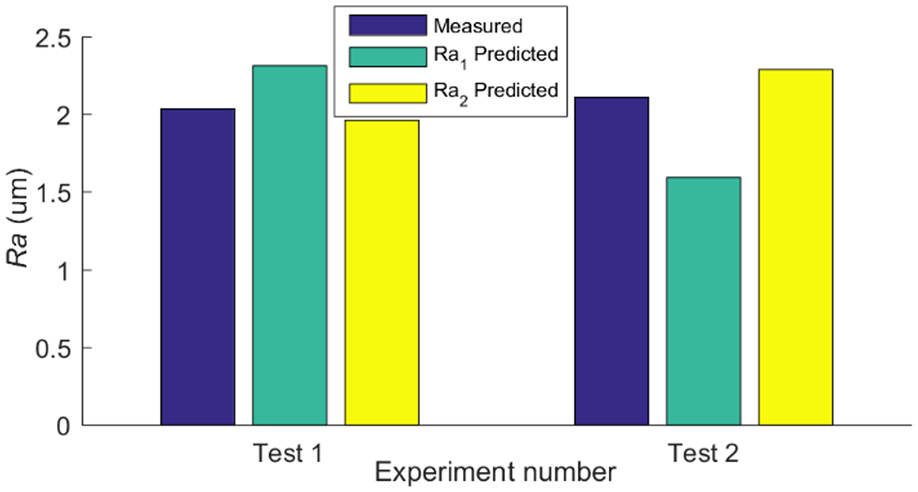
Comparison of prediction accuracy of Ra models.

The SEC measurement results are 3.6144 J/mm³ and 3.2064 J/mm³, respectively. For the test No. 1, the result using SEC₁ is 4.8899 J/mm³ and the prediction accuracy is 64.71%, while the result using SEC₂ is 3.5526 J/mm³ and the prediction accuracy is 98.29%. For the test No. 2, the result using SEC₁ is 3.0401 J/mm³ and the prediction accuracy is 94.81%, while the result using SEC₂ is 3.1419 J/mm³ and the prediction accuracy is 97.99%.

The Ra measurement results are 2.0380 µm and 2.1105 µm, respectively. For the test No. 1, the result using Ra₁ is 2.3178 µm and the prediction accuracy is 86.27%, while the result using Ra₂ is 1.9613 µm and the prediction accuracy is 96.24%. For the test No. 2, the result using Ra₁ is 1.5978 µm and the prediction accuracy is 75.71%, while the result using Ra₂ is 2.292 µm and the prediction accuracy is 91.40%. According to the test results, the developed models SEC₂ and Ra₂ achieve higher prediction accuracy than SEC₁ and Ra₁.

Since the contact between tool and workpiece will certainly initiate tool wear when sufficient cutting time is given, tool wear is unavoidable. Actually, it is an accumulating process including initial, normal, and sharp wear stage. Taking the first cutting insert in this study as an example, the tool flank wear evolution is presented in Figure 14, and the representative SEM images of tool flank wear can be seen in Figure 15. In cutting stage, as the tool flank wear increases, the contact area between tool flank and the machined surface adds. This will lead to an increase in the friction force and cutting temperature between tool and workpiece. More energy is expected to be consumed in cutting stage, and increased surface roughness on the workpiece will be generated.

Figure 14.

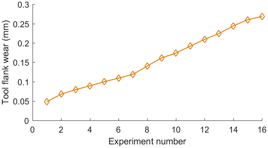
Tool flank wear evolution (taking the first cutting insert in this study as an example).

Figure 15.

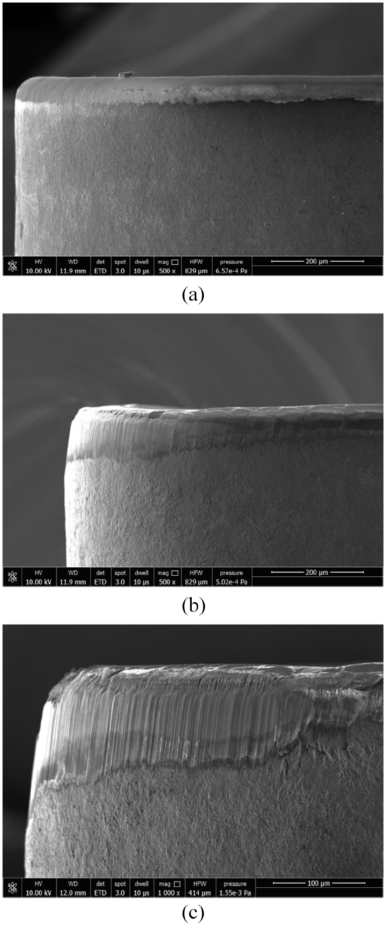
Representative SEM images of tool flank wear: (a) initial wear stage, (b) normal wear stage, and (c) sharp wear stage.

Hence, the effect of tool wear evolution should be taken into account in SEC and Ra modeling. Featuring cutting parameters (a_p, f, and n) and tool flank wear (VB) to establish SEC and Ra models based on SVR algorithm is a more comprehensive and reliable method. This is the reason why the developed models achieve higher fitting accuracy and prediction accuracy.

Conclusion

In this paper, the tool flank wear evolution was observed and recorded in the cutting stage. The SVR models for SEC and Ra based on cutting parameters and tool wear were developed and verified in wet turning AISI 1045 steel experiments. The following conclusions can be drawn.

The tool wear has an important effect on energy consumption of machine tools and workpiece surface quality. Therefore, the wear condition of cutting inserts is a significant factor that cannot be neglected in the modeling of SEC and Ra.

The prediction accuracy of developed models SEC₂ and Ra₂ is 97.99% and 91.40%, respectively. The improved models based on cutting parameters and tool wear are simple with high prediction accuracy, which are useful to formulate cutting parameters that can reduce energy consumption and improve surface quality simultaneously in turning.

Only the tool flank wear is considered in the modeling of SEC and Ra. In addition, the tool rake wear is serious in cutting stage. The effect of tool rake wear on SEC and Ra will be investigated in future.

Footnotes

Appendix A 37

Declaration of conflicting interests

The author(s) declared no potential conflicts of interest with respect to the research, authorship, and/or publication of this article.

Funding

The author(s) disclosed receipt of the following financial support for the research, authorship, and/or publication of this article: This work was supported by the Project of Shandong Province Natural Science Foundation of China (No. ZR2016EEM29) and the Project of Shandong Province key research development of China (No. 2017GGX30114).

ORCID iD

Guoyong Zhao

References

Liu

Wang

Liu

GJ.

Content architecture and future trends of energy efficiency research on machining systems. J Mech Eng 2013; 49(19): 87–94.

Jeswiet

Kara

Carbon emissions and CES™ in manufacturing. CIRP Ann Manuf Technol 2008; 57(1): 17–20.

Gutowski

Dahmus

Dalquist

. Measuring the environmental load of manufacturing processes. In: International society for industrial ecology (ISIE), 3rd international conference, Stockholm, Sweden, 12–15 June 2005.

Zhao

Liu

, et al. Energy consumption in machining: classification, prediction, and reduction strategy. Energy 2017; 133: 142–157.

Zhou

, et al. Energy consumption model and energy efficiency of machine tools: a comprehensive literature review. J Clean Prod 2016; 112: 3721–3734.

Vijayaraghavan

Dornfeld

Automated energy monitoring of machine tools. CIRP Ann Manuf Technol 2010; 59(1): 21–24.

Rao

BC.

Methodology for adapting metal cutting to a green economy. Proc IMechE, Part B: J Engineering Manufacture 2010; 224(8): 1193–1205.

Liu

, et al. An on-line approach for energy efficiency monitoring of machine tools. J Clean Prod 2012; 27: 133–140.

Draganescu

Gheorghe

Doicin

CV.

Models of machine tool efficiency and specific consumed energy. J Mater Process Technol 2003; 141(1): 9–15.

10.

Zhang

Kong

, et al. SEC modeling and influencing trend analysis of cutting parameters. China Mech Eng 2015; 26(8): 1098–1104.

11.

Gutowski

Dahmus

Thiriez

. Electrical energy requirements for manufacturing processes. In: 13th CRIP international conference on life cycle engineering, Leuven, Belgium, 2006, vol. 31, pp.623–638.

12.

Kara

Unit process energy consumption models for material removal processes. CIRP Ann Manuf Technol 2011; 60(1): 37–40.

13.

Kara

An empirical model for predicting energy consumption of manufacturing processes: a case of turning process. Proc IMechE, Part B: J Engineering Manufacture 2011; 225(9): 1636–1646.

14.

Zhou

, et al. An improved cutting power model of machine tools in milling process. Int J Adv Manuf Technol 2017; 91: 2383–2400.

15.

Yan

Xing

ZW.

Energy requirements evaluation of milling machines based on thermal equilibrium and empirical modelling. J Clean Prod 2013; 52: 113–121.

16.

Liu

, et al. Analysis and estimation of energy consumption for numerical control machining. Proc IMechE, Part B: J Engineering Manufacture 2012; 226(2): 255–266.

17.

Axinte

Gindy

Assessment of the effectiveness of a spindle power signal for tool condition in machining processes. Int J Prod Res 2004; 42(13): 2679–2691.

18.

Cuppini

D’errico

Rutelli

Tool wear monitoring based on cutting power measurement. Wear 1990; 139(2): 303–311.

19.

Wan

Chen

, et al. On-line monitoring method of tool wear for NC turning in batch processing based on cutting power. Comput Integr Manuf Syst 2018; 24(8): 1910–1919.

20.

Yoon

Lee

Kim

, et al. Empirical power-consumption model for material removal in three-axis milling. J Clean Prod 2014; 78: 54–62.

21.

Liu

Guo

Sealy

, et al. Energy consumption and process sustainability of hard milling with tool wear progression. J Mater Process Technol 2016; 229: 305–312.

22.

Zhao

Zheng

, et al. Tool tip cutting specific energy prediction model and the influence of machining parameters and tool wear in milling. Proc IMechE, Part B: J Engineering Manufacture 2020; 0954405420911298.

23.

Sofuoğlu

Arapoğlu

Orak

Multi objective optimization of turning operation using hybrid decision making analysis. Anadolu Univ J of Sci and Technology A – Appl Sci and Eng 2017; 18(3): 595–610.

24.

Nas

Öztürk

Optimization of surface roughness via the Taguchi method and investigation of energy consumption when milling spheroidal graphite cast iron materials. Mater Test 2018; 60(5): 519–525.

25.

Zhao

Guo

Zhu

, et al. Energy consumption characteristics and influence on surface quality in milling. Procedia CIRP 2018; 71: 111–115.

26.

Arapoğlu

Sofuoğlu

Orak

An ANN-based method to predict surface roughness in turning operations. Arab J Sci Eng 2017; 42(5): 1929–1940.

27.

Imani

Rahmani Henzaki

Hamzeloo

, et al. Modeling and optimization of cutting force and surface roughness in milling process of Inconel 738 using hybrid ANN and GA. Proc IMechE, Part B: J Engineering Manufacture 2020; 234(5): 920–932.

28.

Debnath

Reddy

QS.

Influence of cutting fluid conditions and cutting parameters on surface roughness and tool wear in turning process using Taguchi method. Measurement 2016; 78: 111–119.

29.

Patel

Gandhi

AH.

Analysis and modeling of surface roughness based on cutting parameters and tool nose radius in turning of AISI D2 steel using CBN tool. Measurement 2019; 138: 34–38.

30.

Kosaraju

Anne

VG.

Optimal machining conditions for turning Ti-6Al-4V using response surface methodology. Adv Manuf 2013; 1: 329–339.

31.

Parida

Maity

Modeling of machining parameters affecting flank wear and surface roughness in hot turning of Monel-400 using response surface methodology (RSM). Measurement 2019; 137: 375–381.

32.

Cortes

Vapnik

Support-vector networks. Mach Learn 1995; 20(3): 273–297.

33.

Lü

Tang

Zheng

Research on data-driven methodology for energy consumption of turning and drilling processes. Comput Integr Manuf Syst 2020; 1–16.

34.

Tong

Liu

Support vector regression and genetic-algorithm-based multiobjective optimization of mesoscopic geometric characteristic parameters of ball-end milling tool. Proc IMechE, Part B: J Engineering Manufacture 2020; 234(10): 1333–1345.

35.

Sofuoğlu

Çakır

Kuşhan

, et al. Optimization of different non-traditional turning processes using soft computing methods. Soft Comput 2019; 23: 5213–5231.

36.

Singh

Guo

. The development of a novel on-line optical inspection system for tool conditions in machining processes. In: Proceedings of the AMSE international manufacturing science and engineering conference, Erie, PA, 12–15 October 2010, pp.607–613. New York: ASME.

37.

Chang

Lin

CJ.

LIBSVM: a library for support vector machines. ACM Trans Intell Syst Technol 2011; 2(3): 1–27.

Prediction models for specific energy consumption of machine tools and surface roughness based on cutting parameters and tool wear

Abstract

Keywords

Introduction

Experimental and SVR modeling details

Experimental design

CNC turning operations

Tool wear and surface roughness measurement

Machine tool power measurement and specific energy consumption calculation

SVR modeling

Running of SVR

Prediction models based on cutting parameters

Prediction models based on cutting parameters and tool wear

Results and discussion

Experimental results

Numerical results

Training results of SVR models

Test results of SVR models

Conclusion

Footnotes

Appendix A 37

Declaration of conflicting interests

Funding

ORCID iD

References