
Abstract
This article intends to provide an efficient modeling and compensation method for the synthetic geometric errors of large machine tools. Analytical and experimental examinations were carried out on a large gantry-type machine tool to study the spatial geometric error distribution within the machine workspace. The result shows that the position accuracy of the tool-tip is affected by all the translational axes synchronously, and the position error curve shape is non-linear and irregular. Moreover, the angular error combined with Abbe’s offset during the motion of a translational axis would cause Abbe’s error and generate significant influence on the spatial positioning accuracy. In order to identify the combined effect of the individual error component on the tool-tip position accuracy, a synthetic geometric error model is established for the gantry-type machine tool. Also, an automatic modeling algorithm is proposed to approximate the geometric error parameters based on moving least squares in combination with Chebyshev polynomials, and it could approximate the irregular geometric error curves with high-order continuity and consistency with a low-order basis function. Then, to implement real-time error compensation on large machine tools, an intelligent compensation system is developed based on the fast Ethernet data interaction technique and external machine origin shift, and experiment validations on the gantry-type machine tool showed that the position accuracy could be improved by 90% and the machining precision could be improved by 85% after error compensation.
Introduction
With the rapid development of the shipping, aerospace, wind power, and nuclear power industries, there has been existed a huge and urgent demand for high-precision and large-scale machine tools. However, the accuracy of machine tools is severely affected by a variety of error sources, such as geometric errors, thermal errors, cutting force-induced errors, servo errors, and tool wear.1–4 And compared with conventional-sized machine tool, large machine tool shares a poorer geometric stiffness and thermal stability due to its large structure, the transverse beam would bend due to its own heavy weight and then results in significant positioning error and straightness error. 5 Furthermore, angular error would also generate significant influence on the spatial positioning accuracy due to the long translational axis. 6 The combined effect of the individual geometric error component within the entire machine workspace is defined as synthetic geometric errors, and they are the major factors to cause the dimensional inaccuracy of the machined features. 7 Therefore, effective identification and compensation of the synthetic geometric errors are quite essential for large machine tools.
During the past decades, a great deal of research work had been conducted on the identification, modeling, and compensation of machine tool geometric errors. Mir et al. 8 analyzed various sources of geometric errors that were usually encountered on machine tools and their effects on the tool-tip position. Khan and Chen 9 proposed an efficient methodology to calculate the position-dependent and position-independent geometric errors of multi-axis machine tools. Raksiri and Parnichkun 10 introduced a back-propagation (BP) neural network-based compensation model for a computer numerical control (CNC) milling machine considering the effects of geometric and cutting force-induced errors. Chen et al. 11 proposed an analytical modeling method to decompose the manufacture errors of a hybrid parallel link machine tool in an inverse kinematic solution. Lei and Hsu12,13 used a probe ball measurement device to identify the geometric errors and their effects on the overall position accuracy of a five-axis machine tool, and the individual error parameter was estimated with least square estimation method. Wang and Guo 14 applied the homogeneous transformation matrix (HTM) to establish the three-dimensional positioning error model for a gear grinding machine, and a laser tracker was adopted to identify the 21 geometric error components. Xiang et al. 15 proposed a generalized volumetric model for multi-machine tools, which can be applied to four types of three-axis machine tools and 12 types of five-axis machine tools. Su and Wang 16 introduced an indirect estimation method to identify the machining accuracy of multi-axis machine tools by probing the factors on an S-shaped test-piece. All the above researches are of great significance in improving machine tool position accuracy. However, most of these researches were conducted on conventional-sized machine tools, and few researches were done about the error modeling and compensation for large-scale machine tools.
To achieve error compensation in the commercial CNC system, the compensation methods proposed before can be mainly divided into two groups: internal interpolation compensation and external software-based error compensation. The former mainly refers to eliminate the machine tool errors by modifying the numerical control (NC) codes.17,18 This compensation method cannot be real-time achieved, due to the time wasted in NC codes modifying, so it is mainly used to compensate the static geometric errors. The external software-based error compensation method is an efficient and cost-effective way to improve machine tool accuracy. It can be used to compensate various types of machine errors, such as linear positioning error, 19 spindle thermal drift error, 20 and cutting force-induced error. 21 And the external compensation system developed before generally read the machine position coordinates and fed back the compensation value through the digital input/output (I/O) module of machine tools. However, the available I/O ports of a machine tool are usually limited, and it would constrain the multi-axis synchronous compensation. So, new compensation technique should be developed for the comprehensive error compensation of multi-axis machine tools. Furthermore, to facilitate the widespread implementation of compensation technique in the workshop, an effective compensation system featured online automatic modeling and an error prediction model with high accuracy are also quite essential.
This article intends to provide an efficient modeling and compensation method for the synthetic geometric errors of large machine tools. In the following section, the major error components affecting machine tool accuracy are identified, and a synthetic geometric error model is established for a large gantry-type machine tool. Then, an automatic modeling algorithm is proposed to approximate the irregular geometric error curves in section “Geometric error measurement and error parameter modeling,” and the angular error’s effect on the machine tool accuracy is introduced thereafter. Finally, an intelligent external compensation system is developed for error compensation in section “Compensation implementation and results,” and some compensation experiments and machining tests were conducted on the gantry-type machine tool to validate the effectiveness of the real-time compensation system.
Synthetic geometric error model of a large gantry-type machine tool
Geometric error parameter definition
Due to the geometric errors arising from manufacturing, assembly defects, and misalignment of the machine tool axes, the actual position of the tool-tip differs from its nominal position and would result in dimensional error of the machined features. And the traditional linear positioning accuracy and repeatability of the translational axes are generally used to evaluate the machine tool accuracy. 22 This specification neglects all other geometric effects such as angular, straightness and squareness errors, which can have a significant effect on the true precision capability of machine tools. In order to provide a comprehensive description of the machine tool spatial error distribution, all the geometric error components affecting the tool-tip position accuracy are analyzed here.
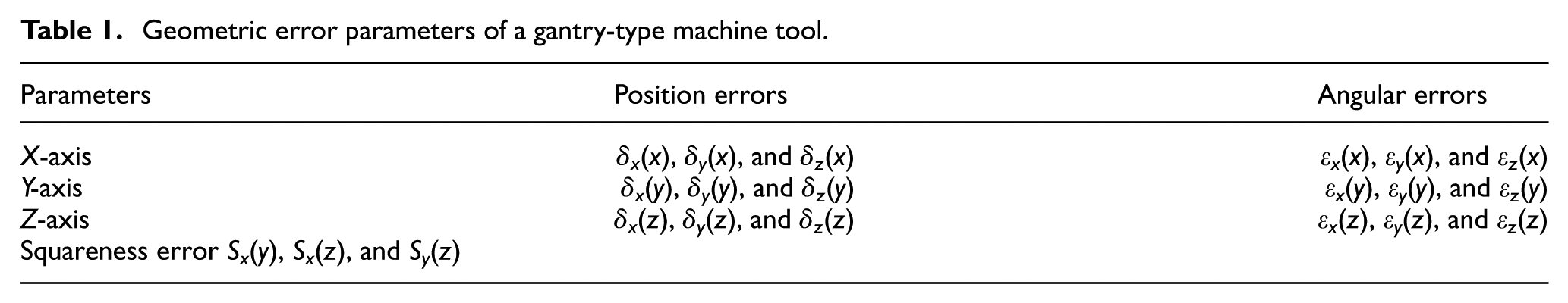
From the perspective of rigid body kinematics, there exist six position-dependent errors when a translational axis moves along a slideway. Taking Y-axis as an example, the six geometric error parameters are shown in Figure 1, including one positioning error, two straightness errors (horizontal and vertical), and three angular errors (pitch, yaw, and roll errors). For a gantry-type machine tool (as shown in Figure 3(a)), all the possible position-dependent error parameters are shown in Table 1. δx(i), δy(i), and δz(i) are the linear position errors of axis i(i = x, y, z), where the first subscript represents the error direction. εx(i), εy(i), and εz(i) are the angular errors of axis i(i = x, y, z), where the first subscript represents the error direction.
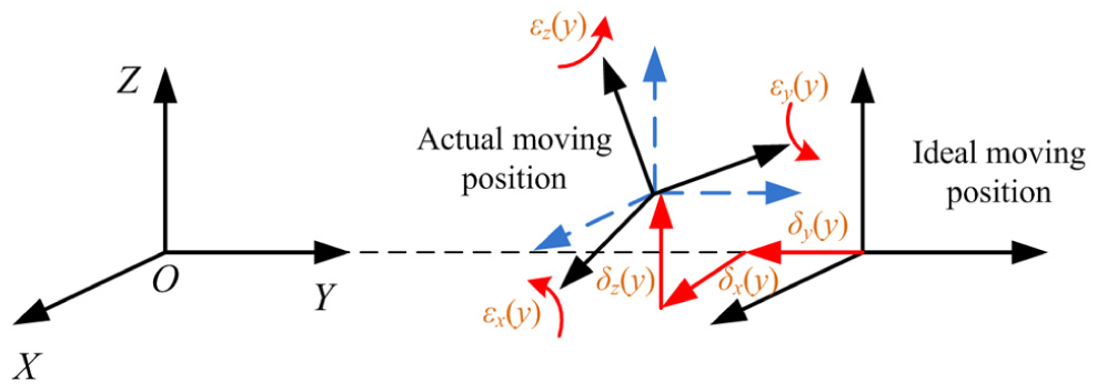
Error parameters of Y-axis.
Geometric error parameters of a gantry-type machine tool.
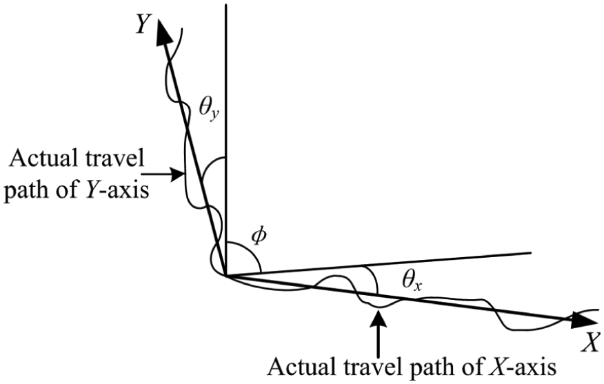
Additionally, there also exists one position-independent error, that is, squareness error, between every two axes. The determination of squareness error Sx(y) between X-axis and Y-axis is shown in Figure 2. The mean straight line of the straightness error curves δy(x) and δx(y) is obtained by applying least square fitting method, and the squareness error can be expressed as follows
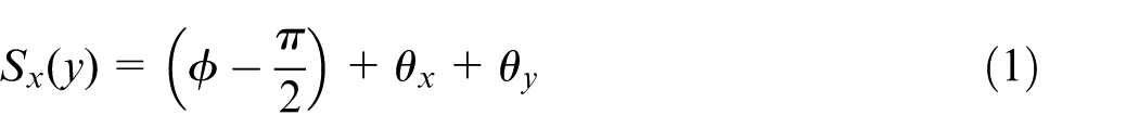
where θx and θy are the calculated angles between the mean straight fitting line and the reference laser beam, φ is the angle between two reference laser beams, which is used to measure the horizontal straightness errors of axes X and Y, and φ − π/2 is the calibration error.
Squareness error between X-axis and Y-axis.
Synthetic geometric error model of the gantry-type machine tool
The structure loop and kinematic chain diagram of the gantry-type machine tool are shown in Figure 3. It can be seen from Figure 3 that the machine tool has two structural chains which contain several components connected in series by prismatic joints. One is the workpiece kinematic chain, which is from the machine base to the workpiece. And the other one is the cutting tool kinematic chain, which is from the machine base to the cutting tool.
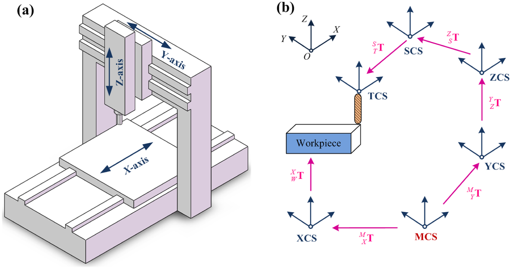
Structure loop and kinematic chain diagram of the gantry-type machine tool: (a) machine structure loop and (b) kinematic chain diagram.
In order to identify the superposition of the error motions of each individual axis on the tool-tip spatial position accuracy, a synthetic geometric error model is established here according to the rigid body assumption and multi-body theory, in which a 4 × 4 HTM is used to represent the transformation relationship between a pair of adjacent bodies. At the nominal configuration, the ideal coordinate transformation for the cutting tool kinematic chain is expressed as follows

where W, X, M, Y, Z, S, and T represent the workpiece, X-axis, machine base, Y-axis, Z-axis, spindle, and cutting tool, respectively;
Similarly, the ideal coordinate transformation for the workpiece kinematic chain is described in equation (3)

In the machining or measurement process, the tool-tip would contact with the workpiece. Thus, the coordinate of contact point on the workpiece coordinate system (WCS) and the tool-tip coordinate system (TCS) is equal in the machine coordinate system (MCS). So, the ideal tool-tip position
where
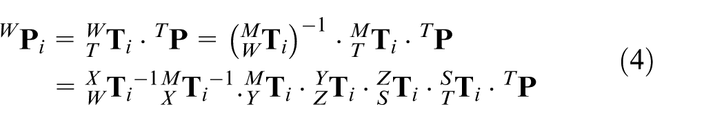
Taking into account of the geometric error influences, the actual tool-tip position
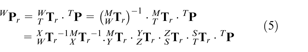
where
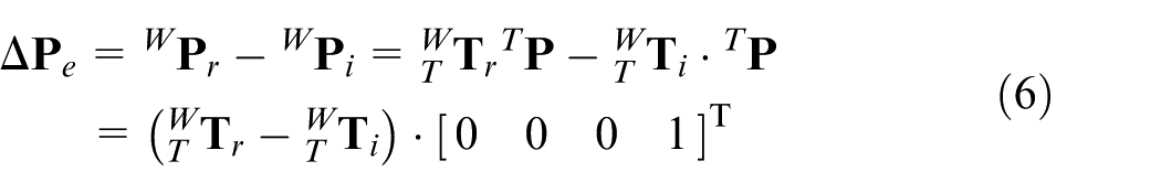
Then, the spatial position error of the tool-tip with respect to the workpiece can be expressed by
In this article, the MCS is selected as the reference coordinate system, and the X-axis is taken as the reference axis of the machine tool. The initial locations of X-axis coordinate system (XCS), Y-axis coordinate system (YCS), and Z-axis coordinate system (ZCS) locate at the same origin of MCS. When X-axis moves along the machine base with a distance x, the ideal HTM and error matrix of X-axis motion are expressed as follows
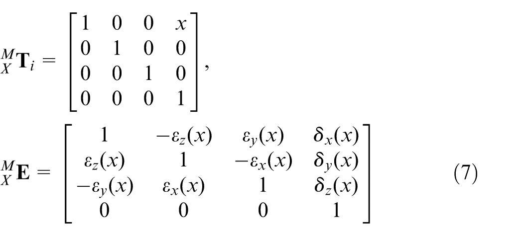
where
So the actual HTM of X-axis motion can be derived as follows
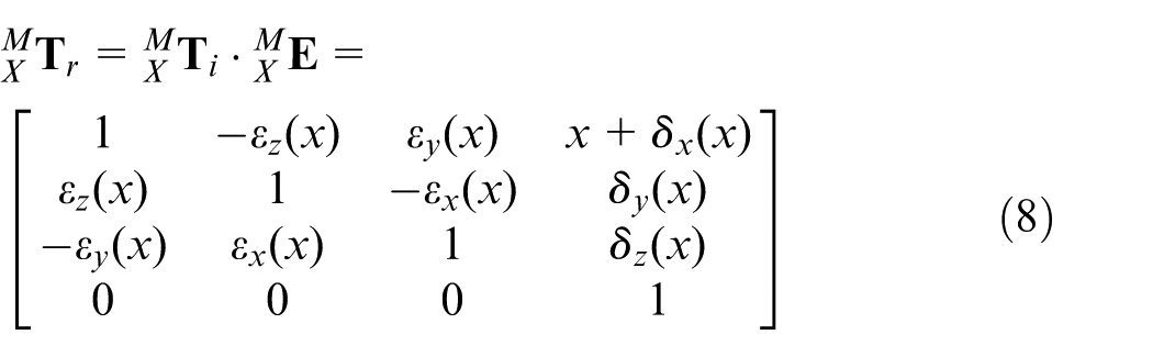
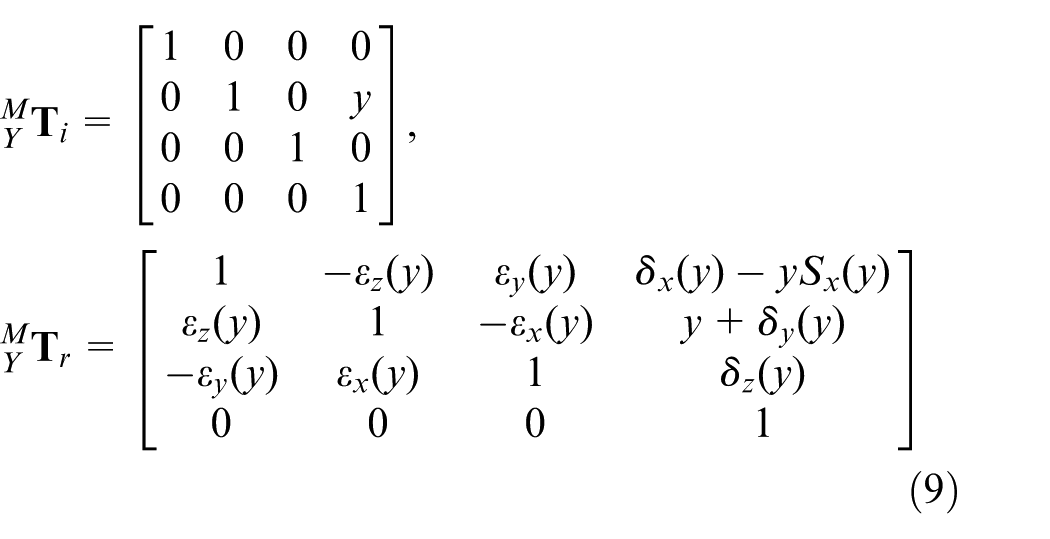
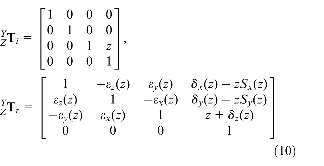
Similarly, the other HTMs can also be obtained as follows
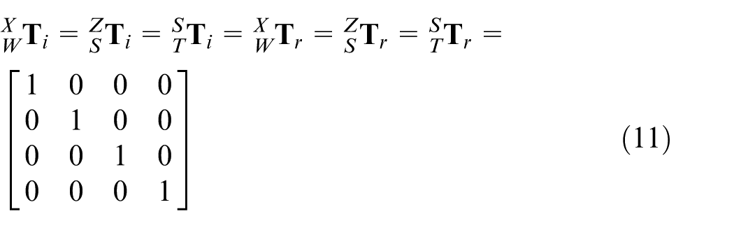
Substituting equations (7), (9), (10), and (11) into equation (4), the ideal transformation matrix
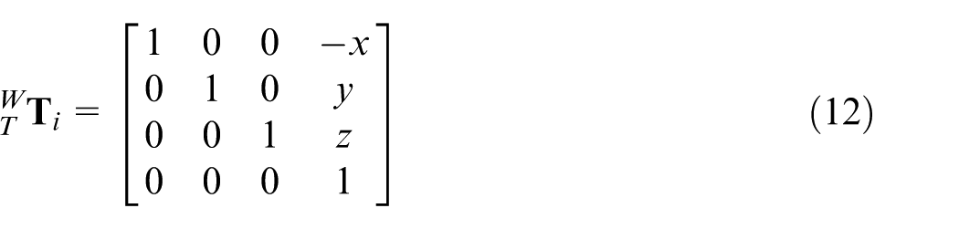
Similarly, substituting equations (8)–(11) into equation (5), and neglecting the second-order terms, the actual transformation matrix
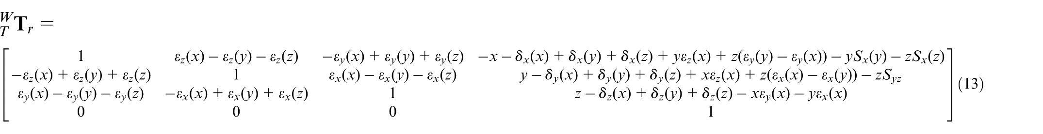
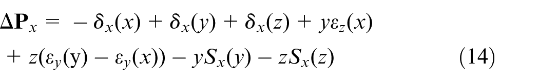
Then, substituting equations (12) and (13) into equation (6), the tool-tip spatial position error
Geometric error measurement and error parameter modeling
Geometric error measurement
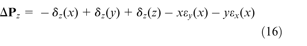
In this research, the measurement experiment was conducted on a large gantry-type machine tool, as shown in Figure 4(a). The structure of the machine tool is XTYZ type. The X-axis is the longitudinal slide which carries the worktable, the Y-axis is the transverse beam which moves perpendicularly to the Z-axis, and the Z-axis is the vertical ram which carries the spindle. The stoke range of the machine tool X-, Y-, and Z-axes are 8000, 4000, and 2500 mm, respectively. And the CNC system is Fanuc 31i.
Measurement experiments conducted on a gantry-type machine tool: (a) tested machine tool and (b) laser measurement of the geometric errors.
In order to identify the error distribution of the gantry-type machine tool, a laser interferometer was used to measure the geometric errors according to the ISO 230-1 measuring criteria, 23 as shown in Figure 4(b). During the measurement process, the starting point was set to be the reference origin of each axis, and 20 measuring points were chosen for each axis. So the X-axis position errors were measured every 400 mm, the Y-axis position errors were measured every 200 mm, and the Z-axis position errors were measured every 125 mm. Meanwhile, the angular measurement method 24 was used here to measure the straightness errors, as its measurement accuracy is superior to the displacement measurement method9,24 for long-stroke machine tool, and less affected by external vibration interference.
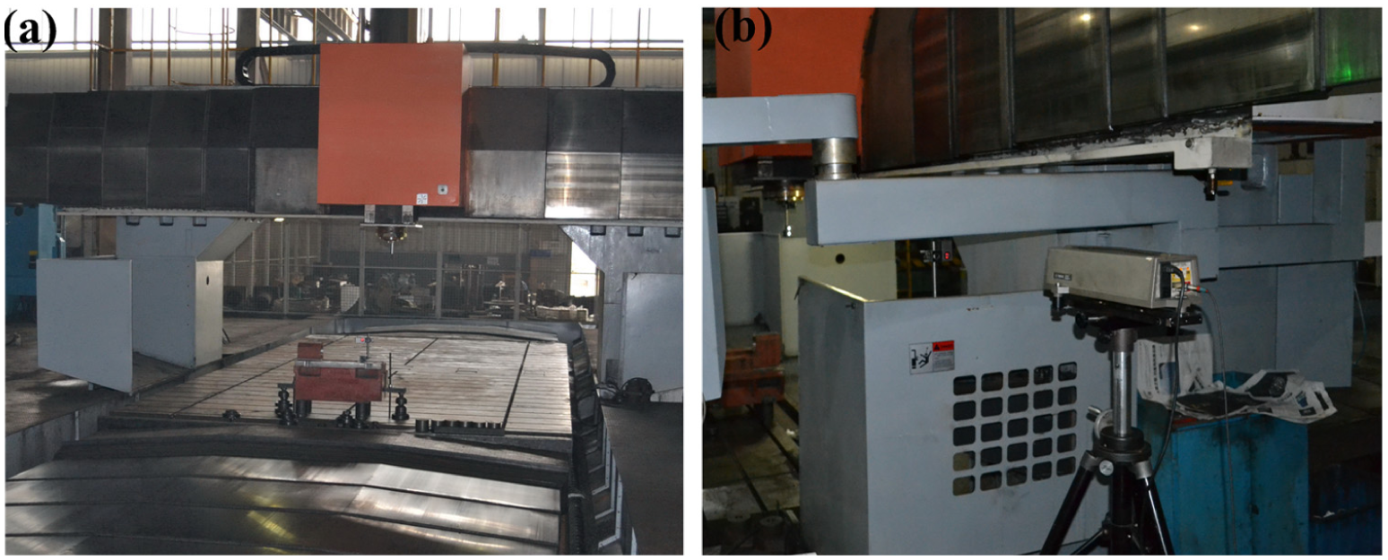
Figure 5 shows the measurement results for the position errors. It can be seen from Figure 5 that as the gantry-type machine tool shares a poorer geometric stiffness and thermal stability due to the large structure, and the transverse beam would bend due to its own heavy weight, it would result in significant positioning error and straightness error. Besides, the geometric error distribution of the gantry-type machine tool is non-linear and the error curve shape is irregular due to the long travel range. To implement error compensation for the gantry-type machine tool, an accurate error model should be established first for the irregular geometric error parameters.
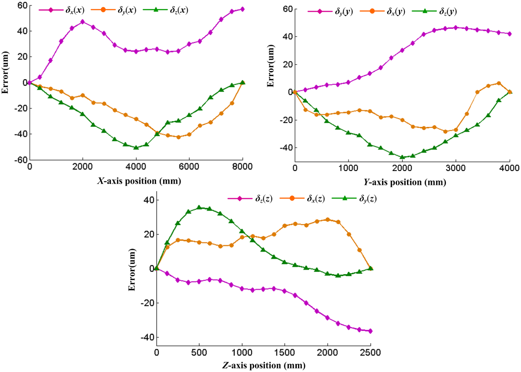
Geometric error distribution of the gantry-type machine tool.
Geometric error parameter modeling based on moving least squares method
Polynomial regression with monomial basis (as shown in equation (17)) was generally used for geometric error approximation. 13 For large machine tools, the error curve shape is usually non-linear and irregular due to its long stroke. High-order polynomials are usually needed to fit the error curve over the entire range. In theory, the approximation accuracy is expected to increase as the order of polynomials increases. However, high-order polynomials usually lead to local over-fitting due to the ill-conditioned Hilbert matrix, subsequently degrade the approximation accuracy

The moving least squares (MLS) approximation is evolved from the ordinary least square method and the corresponding meshless method. This method has been shown to provide better approximation performance for irregular shape curves with its local control ability.25,26 It starts with a weighted least squares formulation for an arbitrary fixed point and then move this point over the entire parameter domain, where a weighted least squares fit is calculated for each measured point individually.
In the MLS approximation, the trial function can be expressed as follows
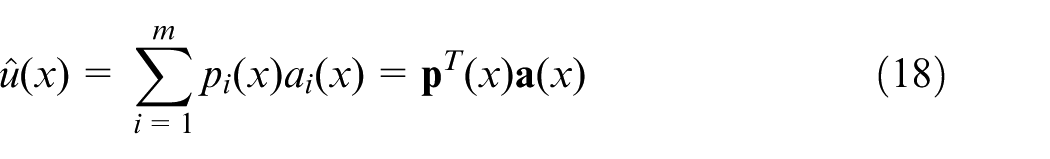
where
For the local approximation at x, a weighted discrete L2 norm is defined as follows
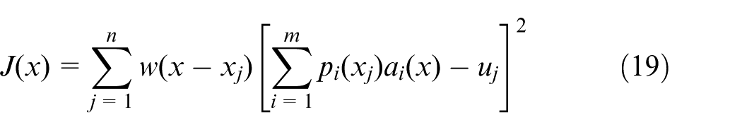
where
Equation (19) could be expressed in matrix as follows

where

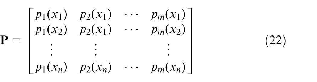
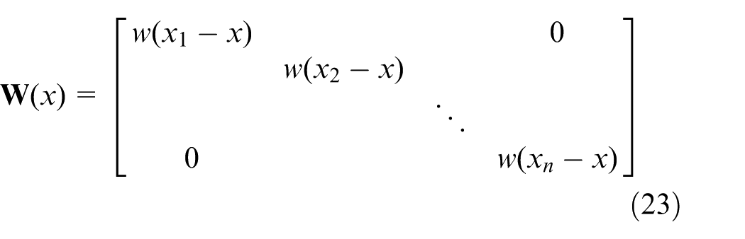
The coefficient vector
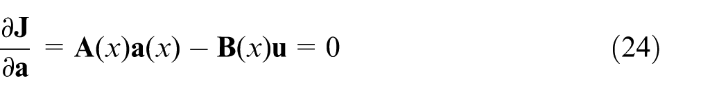
Namely

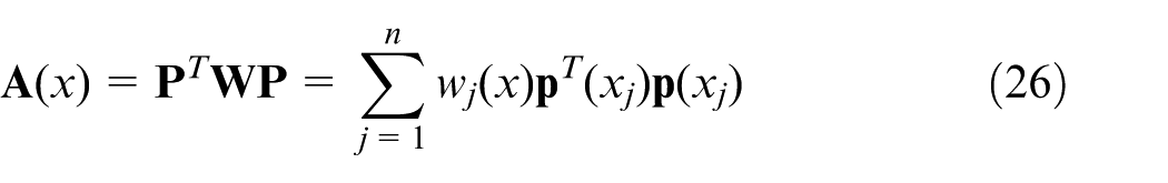
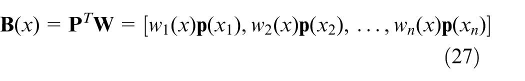
where the matrices
And if we select the basis function and weight function properly so that

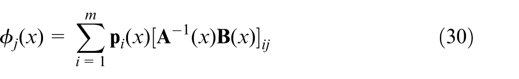
Then, the trail function could be obtained by substituting equation (28) into equation (18)
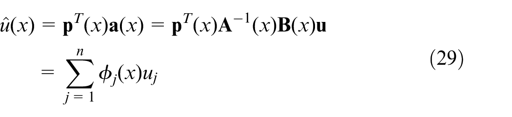
where
The Gaussian weight function is used here to construct the weight function vector
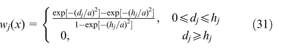
where dj = |x − xj| is the distance from node xj to point x, a is the constant controlling the shape of the weight function, hj is the size of the support for the weight function and determines the support domain of node xj.
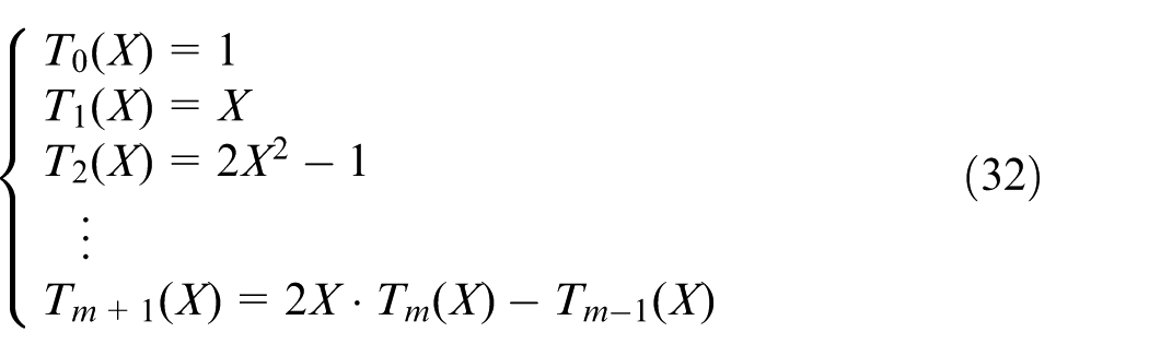
Different polynomials could be used as the basis function, such as monomials, Legendre, and Chebyshev polynomials. Herein, Chebyshev polynomials are chosen to be the basis function, as they have been shown to provide better approximation performance due to their orthogonality,
27
and they contribute the non-singularity of matrix
Chebyshev polynomials of the first kind are defined over [−1, 1], and they satisfy the following recurrence relations
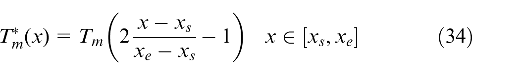
For practical use of Chebyshev polynomials over the interval
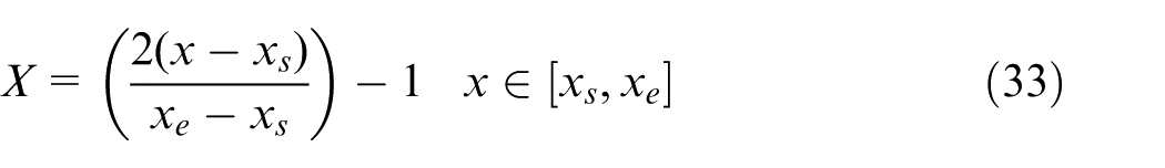
where xs and xe are the starting point and terminal point of the position error measurement interval, respectively.
So, the shifted Chebyshev polynomials
The algorithm flowchart of the error modeling process is illustrated in Figure 6. Meanwhile, in the Gaussian weight function, the shape constant a is set to be 3, and the initial support domain hj is set to be 1/3 of the total range. And the support domain hj and the optimal fitting order of the Chebyshev polynomials could be adjusted according to the modeling accuracy requirement.
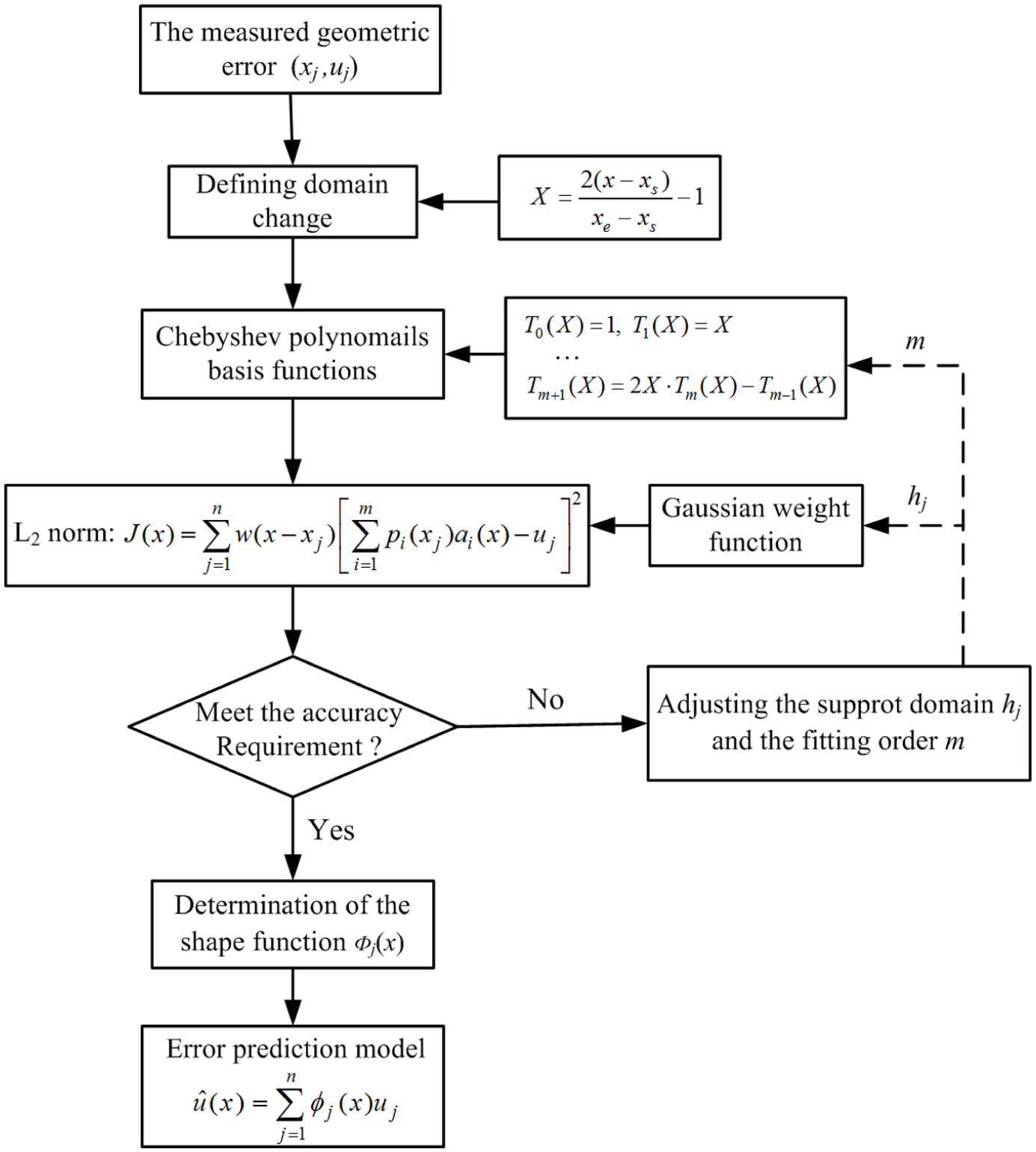
Algorithm flowchart of the moving least squares modeling method.
To validate the modeling accuracy of this modeling algorithm, the MLS with a fourth-order Chebyshev polynomial is used to approximate the X-axis positioning error. And as a contrast, a sixth-order polynomial fitting is also made on the same error curve. The modeling results are shown in Figure 7, and it can be seen from Figure 7 that the modeling residual of the MLS method is −1.4 to 1.7 µm, and the modeling residual of the sixth-order polynomial is −5.2 to 5.0 µm. Additionally, seventh- and higher-order polynomials could still be used to approximate error curve, but the modeling results also turn out to be unsatisfactory due to the local over-fitting. So it can be seen that the approximation performance of the MLS fitting is superior to the polynomial fitting for the irregular shape curves, as it shares a better control of the shape function smoothness and local continuity, then it could achieve better fitting accuracy with low-order Chebyshev polynomials.
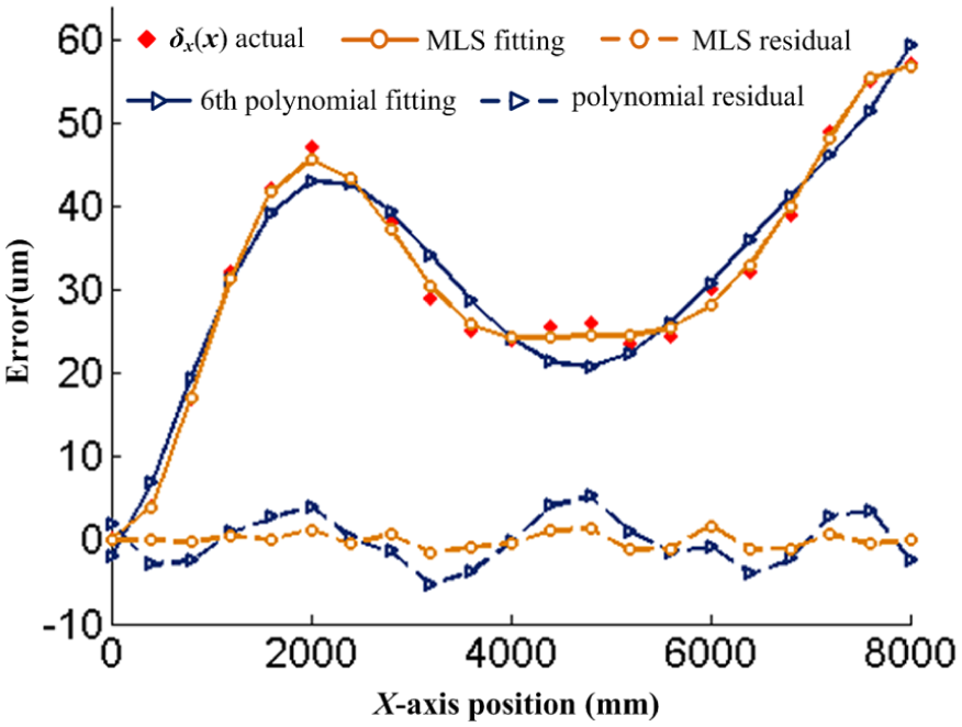
Approximation performance of MLS and polynomial.
Figure 8 shows the fitting results of the X-, Y-, and Z-axes position errors. It can be seen from Figure 8 that the MLS-based modeling method could approximate the geometric error curves accurately, the modeling residuals of X-, Y-, and Z-axes position errors are [−1.6, 1.7 µm], [−1.6, 1.5 µm], and [−1.5, 1.2 µm], respectively, which turn out to be quite satisfactory.
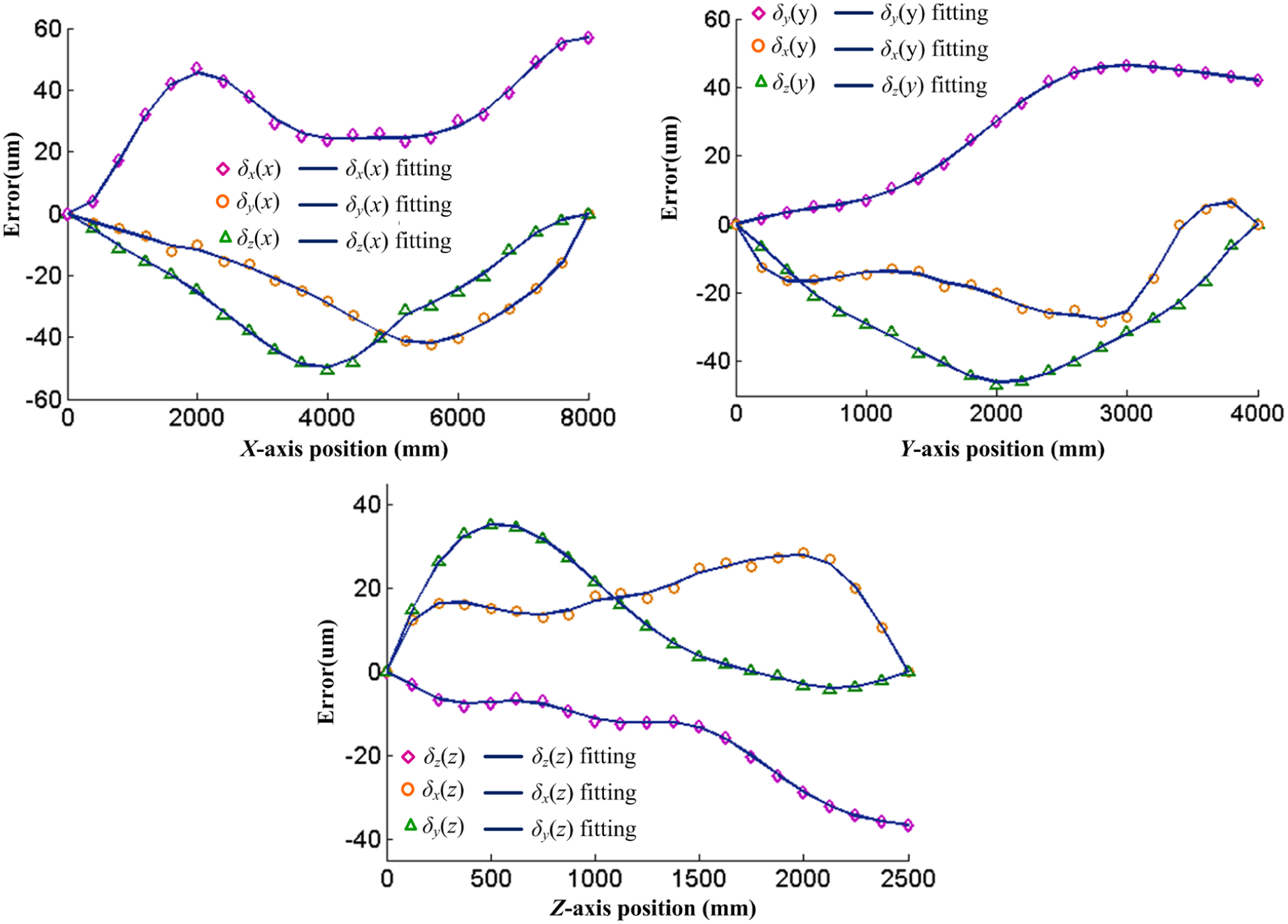
Fitting results of X-, Y-, and Z-axes position errors.
Angular error induced Abbe’s error
It can be seen from the synthetic geometric error model (equations (14)–(16)) that the tool-tip position accuracy is not only affected by the position errors, but also by the angular errors. And the most important influence from the angular errors is the angular error induced Abbe’s error. According to the Abbe’s principle, in the measurement or machining process, the laser beam or the cutting tool-tip should be in line with the reference line of the translational axis, or Abbe’s error would be induced due to the combination of angular error with the Abbe’s offset.23,28Figure 9 shows the schematic diagram of the Y-axis Abbe’s error, which is induced by the pitch error in the vertical plane. It can be seen from Figure 9 that the Y-axis positioning error measured at different Z-axis heights would be different due to the Abbe’s error.
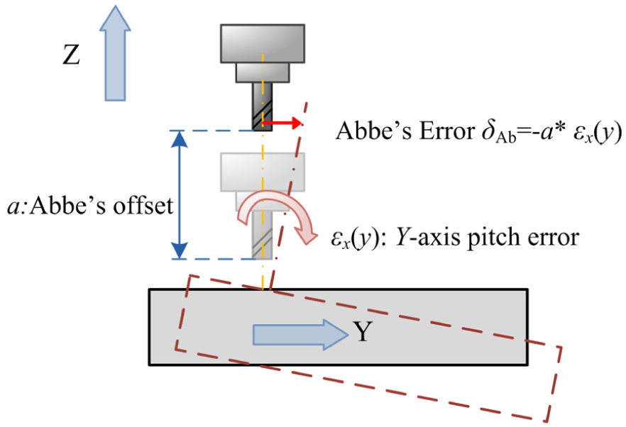
Schematic diagram of the Abbe’s error.
Abbe’s error is an inherent error for all CNC machine tools, as the path of the cutting tool is generally not in line with the reference line. For conventional-sized machine tools, the travel range of the translational axis is relatively short and the angular deviation is small, so the accuracy defection caused by the angular error was generally ignored in the previous error compensation. 7 However, due to the significant angular error and long travel range of the translational axis, the angular error induced Abbe’s error has been found to be one of the major error sources for large machine tools.6,29 So, angular error should be taken into consideration in the compensation implementation for large machine tools.
In theory, there exist angular errors and Abbe’s offsets in two directions for every translational axis. Taking Y-axis for example, there exist pitch error εx(y) and vertical offset a(z) in the Z-axis direction, and yaw error εz(y) and horizontal offset a(x) in the X-axis direction. So, in the laser measurement process, the Abbe’s errors of the X-, Y-, and Z-axes can be expressed as follows 30
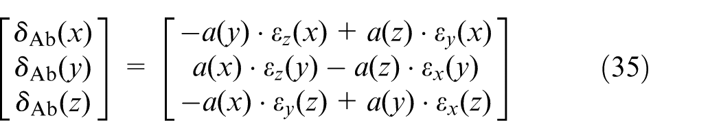
where δAb(x), δAb(y), and δAb(z) are the Abbe’s errors of the X-, Y-, and Z-axes, respectively; a(i) refers to the Abbe’s offset in the i-axis(i = x, y, z) direction.
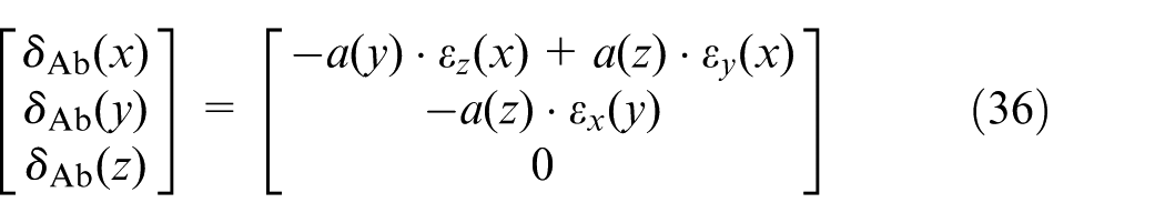
In the actual machining process, as the cutting tool is always collinear with the Z-axis, so there exists no Abbe’s offset for the Z-axis in both the X- and Y-axes directions. Also, the Z-axis slide is mounted on the Y-axis, and there exists no relative movement between the cutting tool and the Y-axis in the X-axis direction, so there is no Abbe’s error for Y-axis in the X-axis direction. However, the cutting tool could move with respect to Y-axis in the Z-axis direction, and with respect to X-axis in both the Y- and Z-axes directions. So, there may exist Abbe’s errors for Y-axis in the Z-axis direction, and for X-axis in both the Y- and Z-axes directions. The Abbe’s errors of the X-, Y-, and Z-axes in the machining process can be expressed as follows
For the gantry-type machine tool in this research, the transverse beam would bend due to its own weight. So there exists angular error in the vertical plane along Y-axis. In the actual machining process, workpieces are usually machined along Y-axis at different Z-axis heights. Then, the occurrence of the Abbe’s offset is inevitable, which would lead to the generation of Abbe’s error due to the combination of angular error with the Abbe’s offset.
In order to identify the Abbe’s error of the Y-axis, a laser interferometer was used to measure the Y-axis positioning error at different Z-axis heights and the corresponding angular error. Figure 10 shows the measurement results of the Y-axis positioning error at different Z-axis heights. It can be seen from Figure 10 that the Abbe’s error caused significant effect on the spatial positioning accuracy, the Y-axis positioning error increased from 23 to 70 µm as the transverse beam extended because of the pitch error. Figure 11 shows the Y-axis angular error in the vertical direction, and it can be seen from Figure 11 that the angular error εx(y) varies with the Y-axis position almost in a linear pattern.
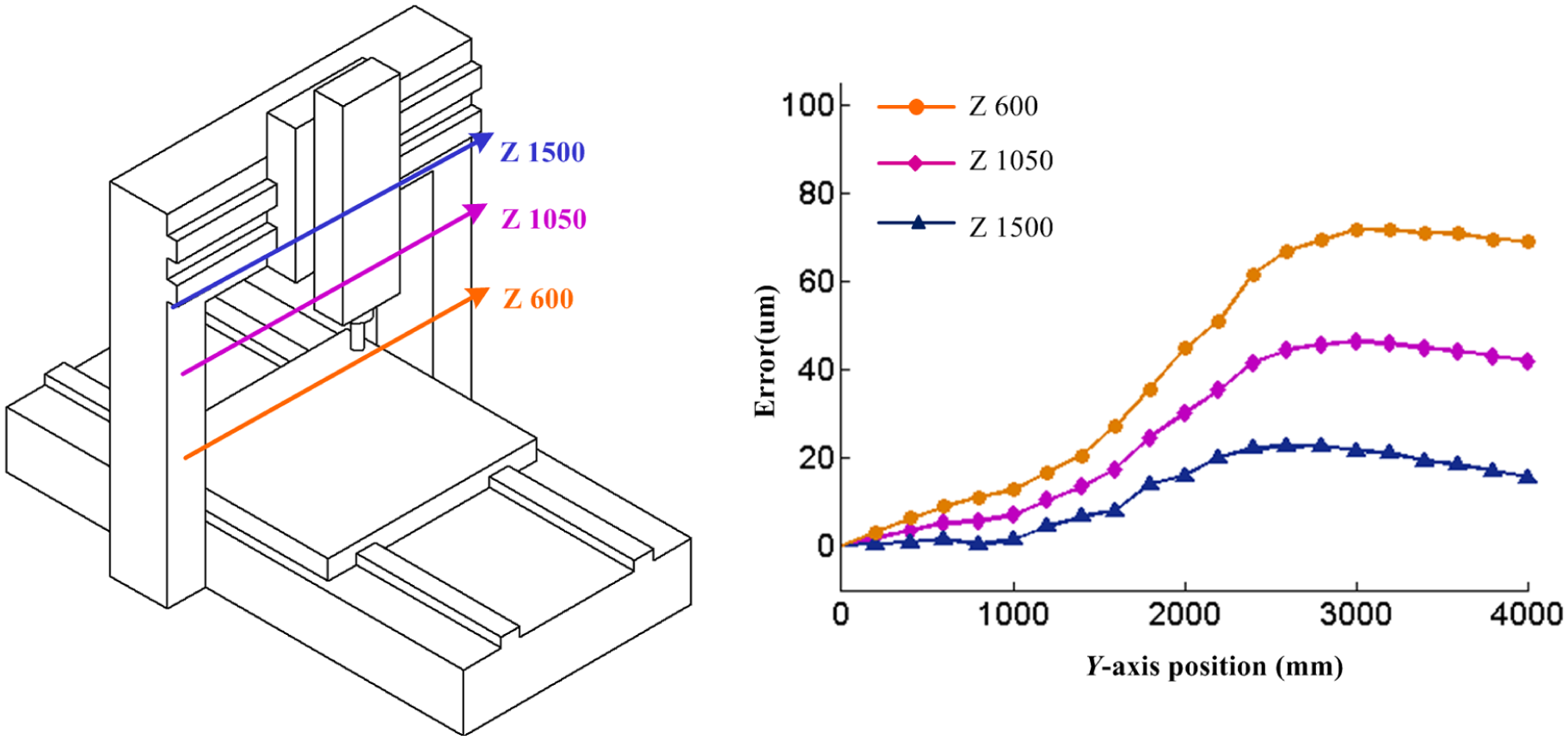
Measurement of Y-axis positioning error at different Z-axis heights.
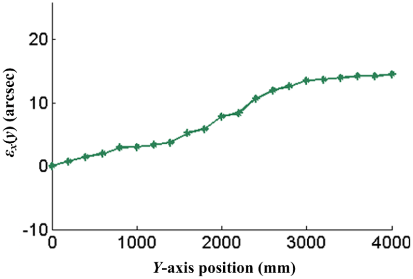
Y-axis angular error in the vertical plane.
Compensation implementation and results
Compensation implementation
The objective of error compensation is to eliminate the motion deviation of the tool-tip at an arbitrary point within the machine workspace. To achieve effective error compensation, apart from an accurate prediction model as discussed above, another key technique is to develop an efficient compensation system. The compensation system developed before generally exchange the position coordinates and compensation value with the CNC system through the digital I/O module. 19 The compensation system read the position coordinates through the DO ports of the I/O module, and the compensation value was fed back to the CNC system through the DI ports of the I/O module, and the data resolution of the digital signal is 1 µm. So, to implement error compensation for a translational axis with a travel range of 1000 mm, and the compensation range is −127 to 127 µm, 15 DO ports and 8 DI ports are needed to fulfill the data transmission requirement. However, the remaining available I/O ports of a machine tool are usually limited, so it would constrain the multi-axis synchronous compensation. This is even more unacceptable for large machine tools with a long travel range, which need more DO and DI ports to fulfill the data transmission.
With the rapid development of Ethernet interaction technique on the CNC system, fast Ethernet data transmission has been realized on some CNC systems. 31 Fanuc 31i CNC system, for example, has achieved a standard fast Ethernet data interaction of 100 Mbps. It has been tested that one compensation cycle could be completed in 8 ms or less, so it could surely meet the compensation requirement of the static geometric errors and quasi-static thermal errors. With the Ethernet interaction technique, the data transmission between the compensation system and CNC system could be completed through the Ethernet, it is quite convenient in the actual implementation. The compensation system developed in this article is based on the fast Ethernet interaction technique.
The compensation system (as shown in Figure 13) consists of hardware platform and software platform, and the schematic diagram of the compensation system is shown in Figure 12. The hardware platform is implemented on an embedded computer, which is connected with the Fanuc 31i system through the Ethernet interface, as shown in Figure 13(b). The mutual data transmission between the compensation system and CNC system is achieved based on the Fanuc Open CNC API Specification (FOCAS) protocol. During each compensation cycle, the compensation system could read the X-, Y-, and Z-axes position coordinates simultaneously through the FOCAS protocol. Meanwhile, the compensation value is also fed back to the CNC system through the FOCAS protocol.
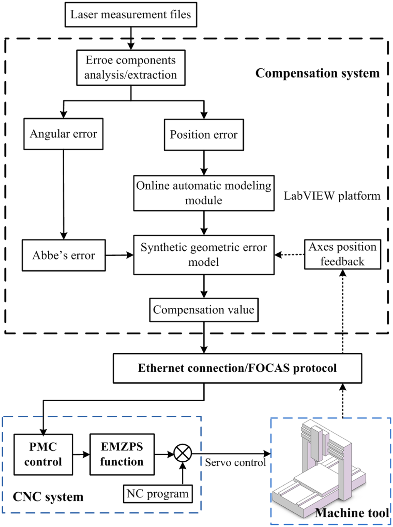
Schematic diagram of the real-time compensation system.
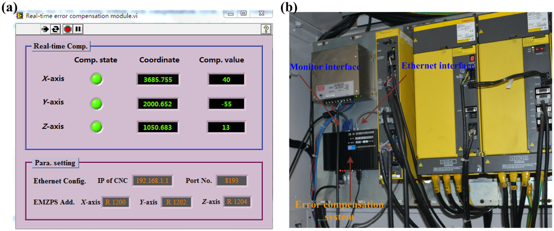
Real-time compensation system: (a) compensation system software platform and (b) compensation hardware installed in the electric control cabinet.
The software platform of the compensation system is developed with virtual LabVIEW, associated with MATLAB procedure, as shown in Figure 13(a). It is mainly composed of two modules, including online automatic modeling module and real-time compensation module. To facilitate online automatic modeling, some MATLAB procedures are embedded in the LabVIEW platform. With the embedded MATLAB procedures, the compensation software could analyze and extract the geometric error components automatically from the original laser measurement files. Then, according to the extracted geometric position error components (positioning error, straightness error, and squareness error), the online automatic modeling module could establish the best fitting algorithm for the position error curves based on the MLS modeling method as presented in section “Geometric error parameter modeling based on moving least squares method.” Also, according to the extracted geometric angular error components, the compensation software could establish the prediction model for the Abbe’s error based on the modeling algorithm presented in section “Angular error induced Abbe’s error.” Finally, according to the volumetric error modeling algorithm in section “Synthetic geometric error model of a large gantry-type machine tool,” a synthetic geometric error model is established for error compensation.
During the actual compensation process, the real-time compensation module would read the position coordinates from the CNC system in every compensation cycle and calculate the tool-tip position error according to the synthetic geometric error model and then send back the compensation value to the CNC system in real time. Then, real-time compensation is carried out in the CNC system based on the function of external machine zero point shift (EMZPS). The EMZPS function could shift the mechanical origin of the feed axes in real time during the machining process. Thereafter, the NC programs would be executed in the modified MCS, and the CNC system sends an additional motion command to the servo control, which is equivalent to the compensation value obtained from the compensation system. Then, the error compensation could be achieved by moving the cutting tool or the workpiece in the opposite direction. It is quite convenient in the actual implementation since it has no interference with the original NC program.
Compensation results
To validate the compensation performance of the real-time compensation system, a series of compensation tests were conducted on the gantry-type machine tool. Figure 14 shows the Y-axis positioning errors measured at different Z-axis heights before and after compensation. It can be seen from Figure 14 that the initial positioning error of Y-axis (Z = 1050) was reduced from 42 to 2.8 µm after error compensation. Affected by the angular error induced Abbe’s error, the Y-axis positioning error measured at Z = 650 increased to 68 µm. After compensation, the maximum positioning error of Y-axis (Z = 650) was also reduced to 4.8 µm. Similarly, Figure 15 shows the measured positioning errors of X- and Z-axes before and after compensation, respectively. It can be seen from Figure 15 that the maximum positioning errors of X- and Z-axes were reduced from 58.6 and 36.6 to 3.5 and 2.7 µm, respectively, after compensation. The positioning errors of the gantry-type machine tool could be compensated by 90%, and the angular-induced Abbe’s error could also be compensated by 75%.
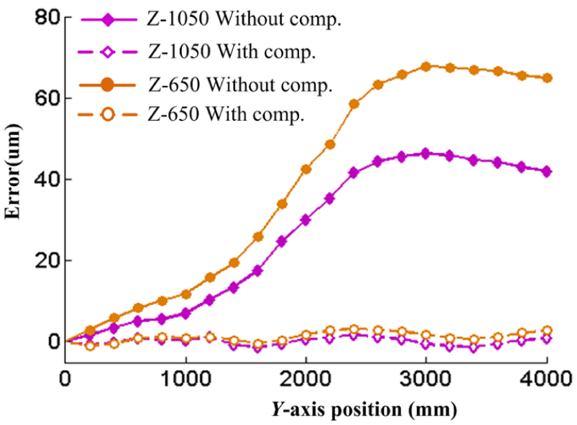
Compensation results for Y-axis positioning errors at different Z-axis heights.
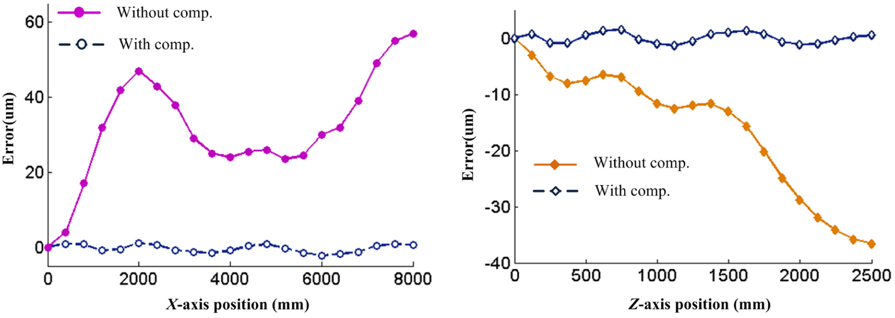
Compensation results for X- and Z-axis positioning errors.
The straightness errors were measured through the angular measurement method in this research, as shown in Figure 4(b). This method has showed high measurement accuracy for long-stroke machine tools and been less affected by external vibration interference. However, the compensation effect of the straightness error could not be validated through the same laser measurement method, 24 and the compensation effect would be reflected on the machined workpieces. Therefore, in order to validate the compensation effect for the straightness errors, some machining tests were conducted on the gantry-type machine tool.
For the machining test, two typical artifacts were machined on the gantry-type machine tool: a machine bed and a worktable. As the surface of the machine bed is used to install guide ways, and the surface of the worktable is used to mount workpieces. So the machining accuracy of these artifacts is very significant, as they have great effects on the accuracy of the machine tools to be produced. The machine bed has a length of 4800 mm in the longitudinal side, and the horizontal and vertical surfaces of the machine bed were both machined with a flat-end milling cutter along X-axis direction as shown Figure 16(a). Then, the X-axis horizontal straightness error δy(x) will be reflected on the vertical plane of the machine bed, and the X-axis vertical straightness error δz(x) will be reflected on the horizontal plane of the machine bed.
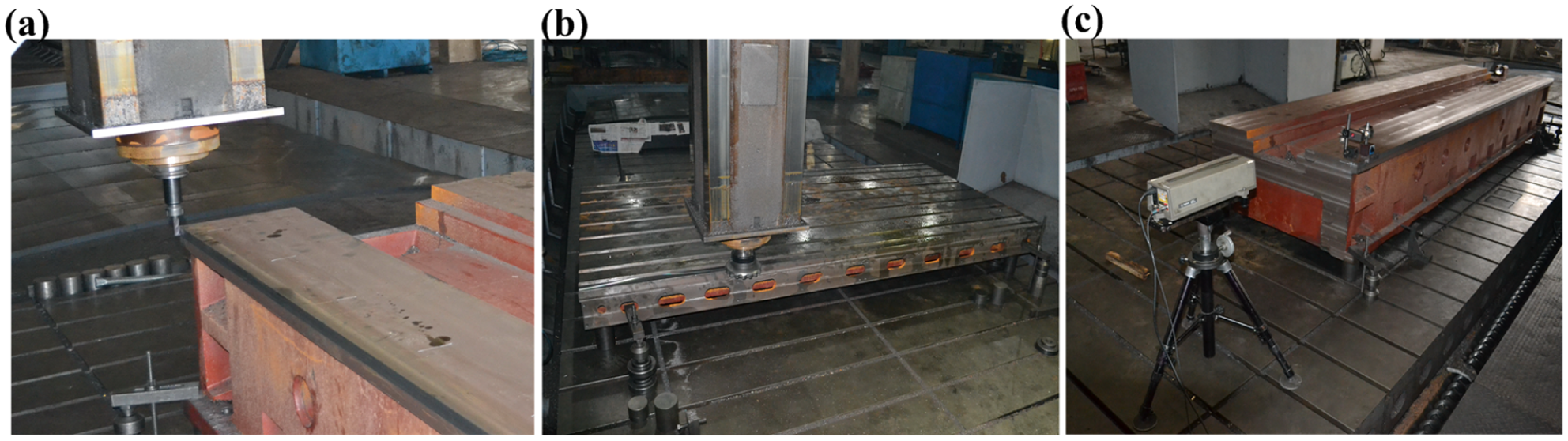
Straightness error measurement with machined workpieces: (a) end milling in X-axis direction, (b) facing milling in Y-axis direction, and (c) measurement of workpiece straightness error.
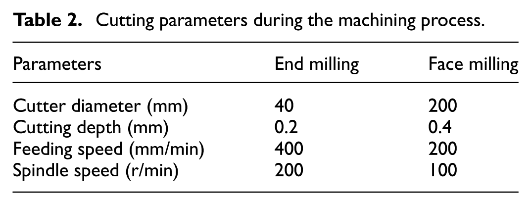
The worktable has a length of 4000 mm in the longitudinal side, the horizontal plane of the worktable was machined with a face milling cutter along Y-axis direction as shown in Figure 16(b), and its vertical plane was machined with a flat-end milling cutter along Y-axis direction. Then, the Y-axis horizontal straightness error δx(y) will be reflected on the vertical plane of the worktable, and the Y-axis vertical straightness error δz(y) will be reflected on the horizontal plane of the worktable. The cutting parameters during the machining process are shown in Table 2.
Cutting parameters during the machining process.
After the machining experiments, the laser interferometer was used to measure the straightness errors of the machined surfaces, as shown in Figure 16(c). The angular reflector was mounted on a bridge plate, which could move on the machined surfaces with a proper interval so that the straightness errors of the machined surfaces could be measured.
Figure 17 shows the measured straightness errors of the machined surfaces before and after compensation. It can be seen from Figure 17 that the X-axis horizontal straightness error δy(x) was reduced from 19 to 3.5 µm, and the X-axis vertical straightness error δz(x) was reduced from 33 to 5.2 µm after error compensation. The Y-axis horizontal straightness error δx(y) was reduced from 34 to 4.6 µm, and the Y-axis vertical straightness error δz(y) was reduced from 50 to 6.8 µm after error compensation. The straightness errors of the machined workpieces could be compensated by 85%, and the machining precision of the gantry-type machine tool was improved significantly after error compensation.
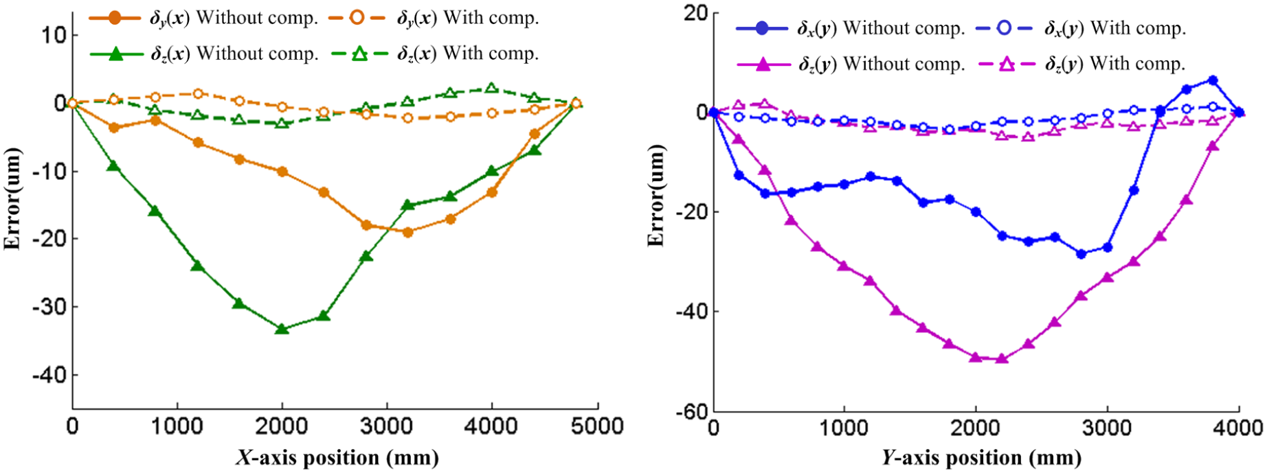
Compensation results for the workpiece straightness errors.
Conclusion
This article provides an efficient modeling and compensation method for the synthetic geometric errors of large machine tools. In order to identify the combined effect of the individual error component on the tool-tip position accuracy, a synthetic geometric error model is established. And an automatic modeling algorithm is proposed to approximate the irregular geometric curves based on MLS method. Then, an efficient compensation system is developed based on the fast Ethernet data interaction technique, and the compensation tests on the gantry-type machine tool showed that the position accuracy could be improved by 90% and the machining precision could be improved by 85% after error compensation. The following conclusions can be drawn.
A synthetic geometric error model is established to predict the spatial position error of the gantry-type machine tool. Except for the previous positioning error and backlash error, the other significant error parameters, such as straightness error and angular error, are also taken into consideration in the compensation process. Hence, the compensation model could achieve better compensation performance in the actual implementation.
An automatic modeling algorithm is proposed to approximate the irregular geometric error curves based on MLS in combination with Chebyshev polynomials. Compared with the general approximation method with polynomials, the advantage of the MLS approximation is that it could obtain the shape function with high continuity and consistency with a low-order basis function, so it is quite suitable for irregular error curve fitting.
The angular error combined with Abbe’s offset during the motion of a translational axis would cause Abbe’s error and generate significant effect on the spatial positioning accuracy for large machine tools. So, the angular error induced abbe’s error should be taken into consideration for large machine tools in the compensation implementation.
An intelligent compensation system featured online automatic modeling is developed for machine tools based on the fast Ethernet data interaction technique and external machine origin shift. Compared with the original compensation method based on I/O module, this compensation technique has shown great advantages in terms of multi-axis synchronous compensation and convenient application. Furthermore, the compensation system can also be used to compensate the time-varying thermal errors in the further research.
Footnotes
Appendix 1
Declaration of Conflicting Interests
The author(s) declared no potential conflicts of interest with respect to the research, authorship, and/or publication of this article.
Funding
The author(s) disclosed receipt of the following financial support for the research, authorship, and/or publication of this article: This work was funded by the National Science Foundation Project of P.R. China (No. 51275305, No. 51175343), the Shanghai Municipality Military and civilian projects for the construction of industrial development system (No. JMJH2013002), the Liaoning Province Scientific and Technical Innovation Key Special Projects (No. 201301001), and the Shanghai Municipality Minhang District Industry-University-Research Cooperation Projects (No. 2013MH111).