
Abstract
There are many researches in scheduling an optimal feedrate profile under various constraints by numerical calculation. A large number of discrete feedrate data points are obtained. They are inconvenient for the parametric interpolator. Therefore, these discrete feedrate data points need to be fitted by parameter curves. Different from the regular curve fitting, the inappropriate feedrate fitting method can generate larger acceleration and jerk that seriously affect the machining accuracy and stability, although the feedrate satisfies the error requirements. In order to generate a suitable feedrate profile, a segment feedrate profile fitting method using B-spline is proposed in this article. The discrete feedrate data points are segmented in the jerk discontinuous points. In each segment, the feedrate profile is fitted by the linear least squares method. These fitted feedrate profiles are combined to generate a unified feedrate profile. The unified fitted feedrate profile and the tool path trajectory are used in the controller to command the axis. In this article, the process of parametric interpolation is separated into the arc-length calculation process and the curve parameter calculation process. Using parallel computation, the two processes are calculated simultaneously in the controller, and the computational efficiency is improved. Both simulation and experiment are carried out to verify that the fitted feedrate profile satisfies the error requirements, and the novel interpolation can be applied to the controller appropriately.
Introduction
Machining aerospace parts, biomedical components, and optical lens composed of complex sculptured surfaces at high feedrate motivate much research in the feedrate scheduling and parametric interpolation. Contrast with linearizing the tool path, the parametric interpolation is widely applied for machining the complex sculptured surfaces due to the high precision and efficiency. But there are still many problems that need to be solved in parametric interpolation.
The tool path curves and feedrate profiles are scheduled according to the machine tools and machine process. Many scholars devote to plan an appropriate tool path trajectory1–5 in which the trade-off between the precision and efficiency needs to be handled properly, and to generate an optimal feedrate profile6–13 which is time-optimal under various constraints. For the complexity of the computation, these processes are almost scheduled offline.
For the offline feedrate scheduled method, some researchers define the equation of the feedrate profile and obtain the optimal results by optimizing the parameters of the feedrate profile equation, as shown in Figure 1(a). Altintas and Erkorkmaz 6 use quintic spline representing the feedrate profile and improve the processing efficiency by optimizing the parameters of the quintic spline. Sun et al. 7 and Sencer et al. 8 preset the equation form of the feedrate profile, and the B-spline is chosen to represent the feedrate profile. They adjust the control points of the B-spline to obtain an optimal feedrate profile which satisfies the constraints. In order to achieve the optimal solution, some researchers do not define the curve equation form of the feedrate profile. They find the optimal solution in all the function space, as shown in Figure 1(b). Erkorkmaz et al. 9 propose an intelligent heuristic rules in an optimal process. Fan et al. 10 develop an efficient convex optimization method to address the time-optimal feedrate planning problem with complex constraints. But they do not describe how the optimized feedrate is applied in the parametric interpolation in detail. Beudaert et al. 11 and Lu et al. 12 obtain an optimal feedrate by the iterative method and predictive method. Bharathi and Dong 13 incorporate many constraints into a computationally efficient two-pass algorithm to generate a minimum time feedrate profile. The result is a series of discrete points. It is inconvenient for parametric interpolation, and the feedrate data points need to be fitted by curves. The inappropriate feedrate fitting method may not only deteriorate the optimized feedrate results, but also induce additional larger acceleration or jerk. A segment feedrate profile fitting method is proposed in this article.
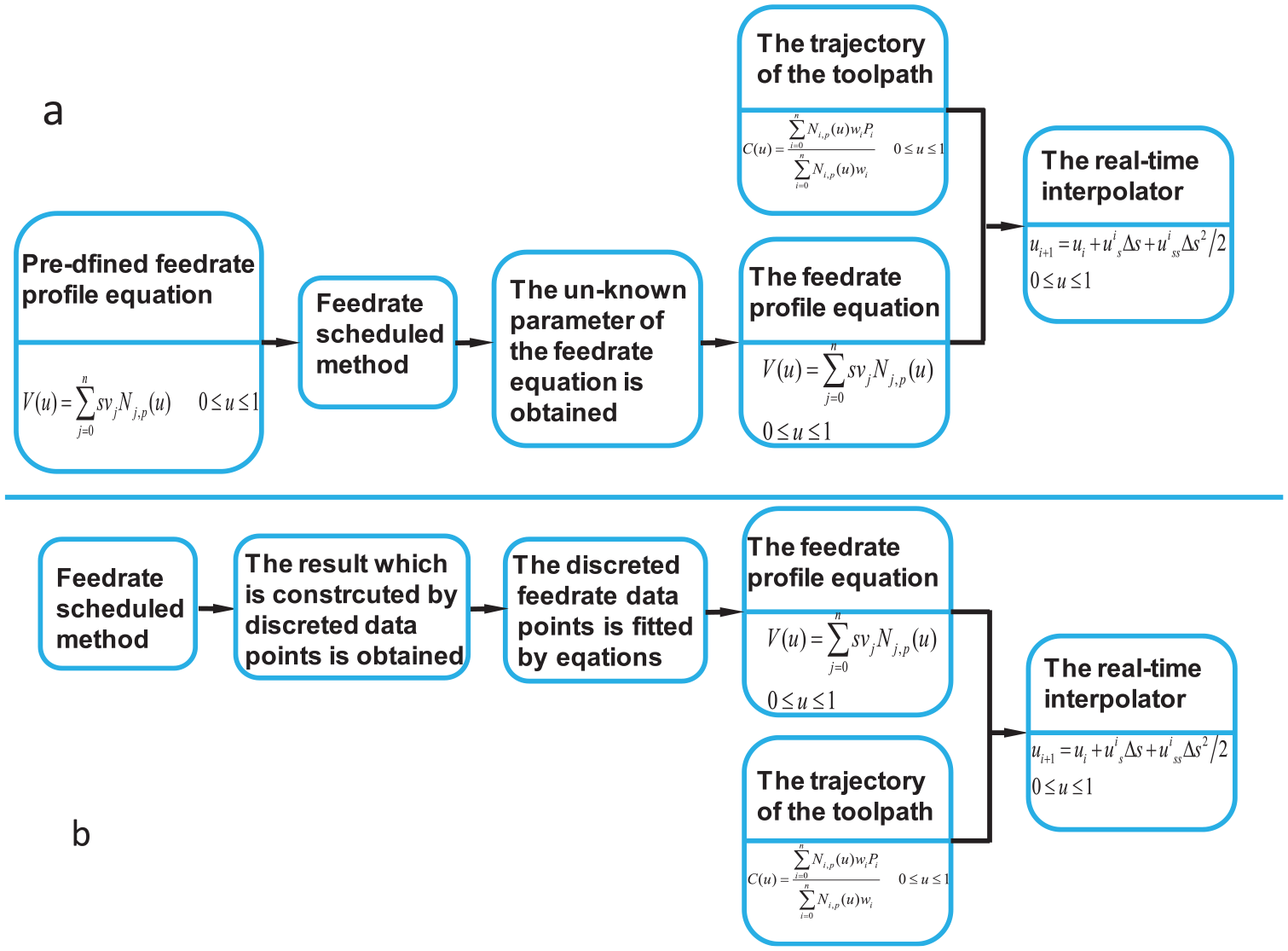
Offline feedrate scheduling process.
After the tool path and feedrate profile are scheduled, these need to be applied in the controller to control the drives. For most of the parameter curves, there is no analytical relationship between arc-length and curve parameter, and at the same time, the computing capability of the controller is limited. Therefore, it is a tough and meaningful thing to calculate the accurate point’s parameter in real time according to the feedrate or arc-length. The Taylor’s expansion method14–22 has been popularly adopted for the parametric interpolation, and the first and second derivatives of the curves need to be computed in real time. For most of the parameter curves, it is time-consuming. Besides the Taylor’s expansion method, the offline mapping of relationship between the arc-length and the curve parameter is also a feasible and effective method,23–30 which releases the computational load of the controller. But the feedrate fluctuations are sensitive to the fitting error between the curve parameter and the arc-length. Apart from the above two methods, the predictive–iterative method31–34 is also used to find the new point’s parameter. Finally, the controller calculates the positions of the new interpolation points and transmits them to the servo axis after kinematics transformation.
Due to the high machining requirements of the free-form surfaces, the feedrate needs to be scheduled using numerical calculation. But the feedrate profile after scheduling is constructed by discrete points and it is inconvenient for parametric interpolation. Therefore, these feedrate data points need to be fitted by curves. Different from the conventional curve fitting, it not only requires the feedrate calculated by the fitted curves to satisfy the error requirements, but also requires the acceleration and jerk to satisfy the error constraints. There are few articles illustrating the fitting method of the feedrate profile in detail. In order to obtain a proper feedrate profile, this article proposes a segment fitting method of the feedrate profile using B-spline. According to the characteristic of feedrate profile and the cubic B-spline, the feedrate profile is split in the jerk discontinuous points. To avoid the nonlinear problem, the knot vectors in each segment are also pre-computed according to the change of the third derivative of the curve in each segment, and the control points that are the unknowns are solved using the linear least squares techniques. After each segment feedrate profile is fitted, a whole feedrate B-spline is obtained by compounding every segment.
As the second-order Taylor expansion is used as the interpolation equation, the us and uss (the first- and second-order derivatives of the parameter respect to the arc-length) need to be calculated in real time, and the computation is time-consuming. In order to improve the computing efficiency, the calculating process is separated into two computing process in this article: the arc-length calculation process and the curve parameter calculation process. The calculation capability of the interpolation is improved using the parallel computation.
The remainder of this article is organized as follows. The tool path planning and the segment feedrate profile fitting method are illustrated in section “Tool path planning and feedrate profile fitting.” In section “Parametric interpolation,” a novel parametric interpolation method is developed. The simulation and experiment are conducted in sections “Simulation” and “Experiment,” respectively. Finally, conclusions are drawn in section “Conclusion.”
Tool path planning and feedrate profile fitting
Tool path planning
As shown in Figure 2, the tool path is planned according to the machining process, and the shapes of the tool and workpiece. The equation form of the tool path needs to be modulated according to the interpolator under the error requirements.
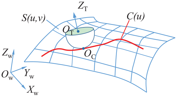
Tool path planning.
In this article, the tool path is represented by the non-uniform rational B-spline (NURBS) curve. A NURBS curve C(u) can be defined as
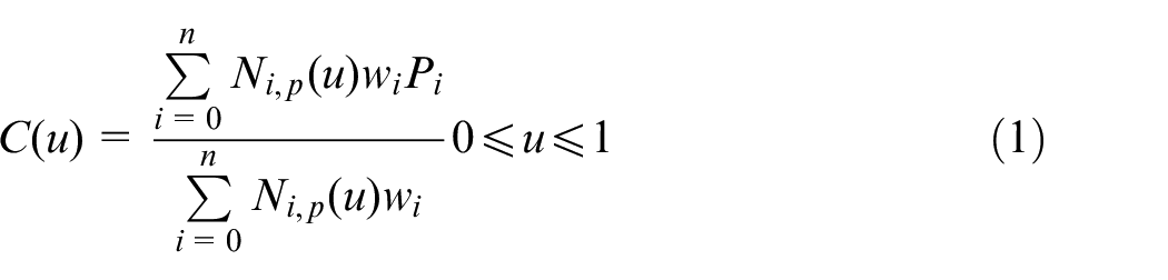
where Pi is the control point, wi is the corresponding weight of Pi, and
Segment fitting of feedrate profile
For machining process, the feedrate of the tool respect to the workpiece not only has great influence on the machine efficiency but also affects the machining precision. At the same time, the limited drive ability of the machine constrains the axial velocity, acceleration, and jerk. Therefore, identifying a feedrate profile which the trajectory is executed in minimum time without exceeding the capabilities of the actuators is a non-trivial optimal process problem
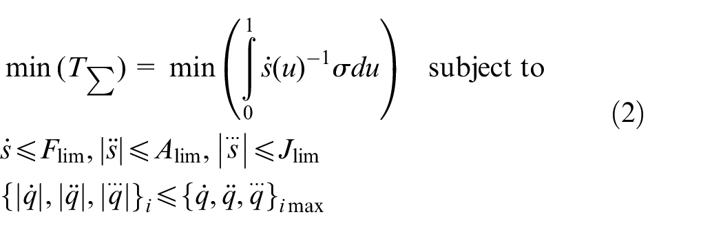
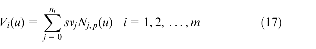
where
Dividing the feedrate profile
After the feedrate profile is scheduled using numerical calculation, a series of feedrate discrete data points in every tool path’s parameter (i.e.
where
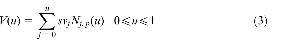
Using the formula for the derivative of the composition of two functions, the first, second, and third derivatives of the feedrate profile to the parameter yield
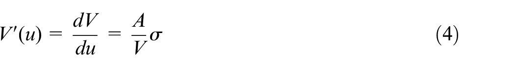
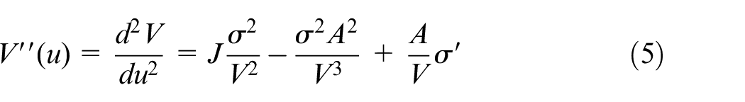
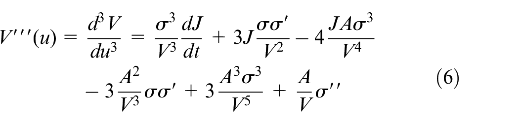
where V, A, and J are the feedrate, acceleration, and jerk of tool respect to the workpiece;
The jerk is arbitrary and discontinuous in most of the feedrate scheduling process for it is considered as the highest order constraints. According to the characteristics of the B-spline, the continuity of the B-spline in the knot is Ck − r, 35 noting that k is the degree of the B-spline, and r is the multiplicity of the knot. Therefore, the feedrate profile is split according to the jerk, and a cubic B-spline is fitted to the feedrate profile data.
According to the characteristics of the cubic B-spline, the second derivative
Determining the knot vector of the feedrate profile
How many knots are required to obtain the desired accuracy is not known in advance, and therefore, the approximation methods are generally applied iteratively in each segment. The knot vector in each segment is determined as follows:
Start with the minimum number of the knots;
Fit an approximating curves to the data using a global fit method;
Check the errors between the curve and the data;
If they satisfy the error requirements, return; otherwise increase the number of the knots and go back to Step 2.
After the number of the knots is determined, the knots need to be distributed over the segment properly. According to the characteristics of the cubic B-spline, the third derivative of the curve
Calculating the control points of the fitted B-spline
Due to the feedrate in every tool path points
is sought in the i-segment of the feedrate profile satisfying that:
The remaining feedrate points
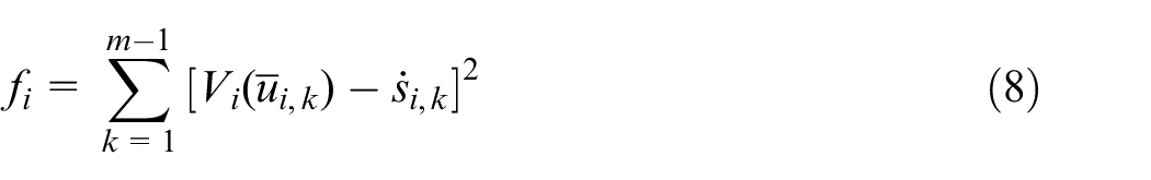
is a minimum with respect to the n + 1 variables,
Let the
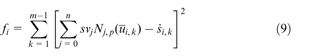
The multiplicity of the first and last knots is 4 in the open knot vector, and the fitted curve passes through the first and last control points, that is

Then
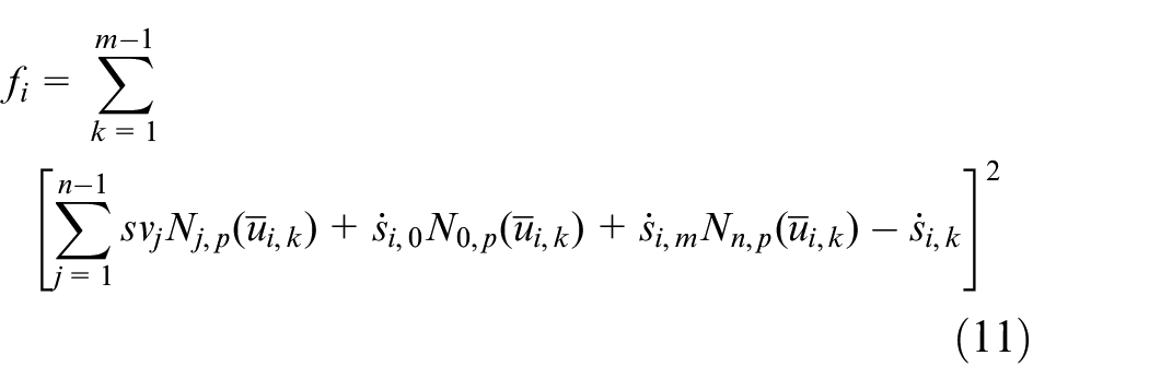
fi is a scalar-valued function of the n − 1 variables,
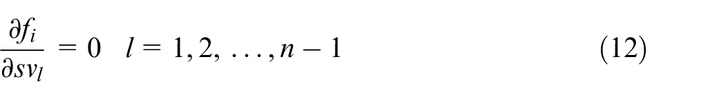
which implies that
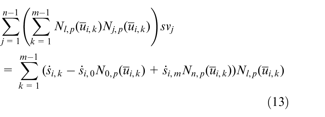
where
Letting

where N is the
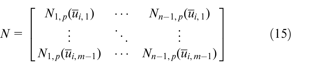
NT is the transport matrix of N, and R is the vector of n − 1 points
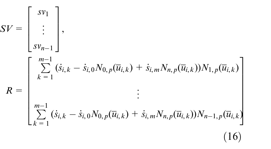
Equation (14) can be solved by Gaussian elimination without pivoting.
Compounding the B-spline
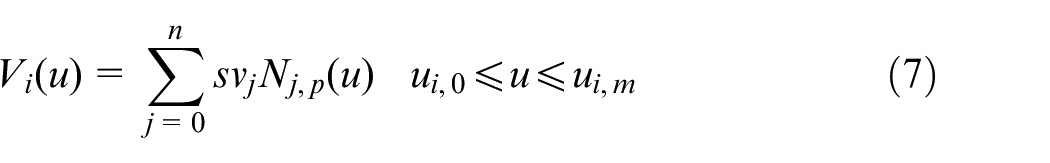
After each feedrate profile segment is fitted, these divided B-splines are still inconvenient for the parametric interpolation. Therefore, they need to be composited to a whole cubic B-spline. The fitted feedrate profile curve in the ith segment is
1. Determine the control points
where
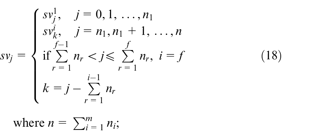
2. Determine the knot vector
Parametric interpolation
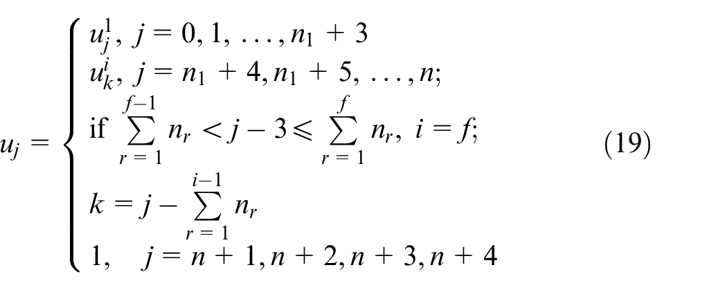
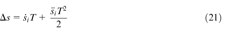
According to the scheduled feedrate profile and the interpolation period T, the arc-length is calculated by the feedrate and acceleration in the current point ui
where
Many parametric interpolation methods can be used to calculate the next interpolation parameter
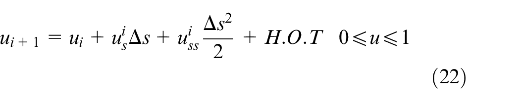
where
According to the parametric interpolation process, the feedrate and acceleration in every trajectory point need to be calculated for obtaining the arc-length in every interpolation period. The feedrate is acquired by the fitted feedrate B-spline profile, and the acceleration can be obtained by the differential calculation method. And at the same time, the trajectory point in the parameter ui, and the
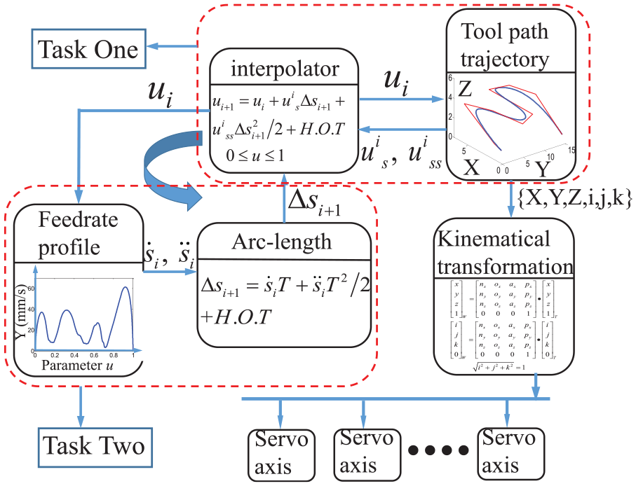
Parallel interpolation process.
As shown in Figure 3, in the process of task one, the calculation of the interlator and the new NURBS trajectory point is processed. The new trajectory parameter ui is obtained by interlator equation as shown in equation (22), and the new trajectory point {X, Y, Z, i, j, k}
i
is computed by the parameter ui in the task one process. As the
In the process of task two, the arc-length is calculated. First, the feedrate in the new trajectory point is calculated according to fitted feedrate cubic B-spline, and the acceleration is obtained by different calculations of the feedrate. At last, the arc-length which is ready for the next interpolation cycle is calculated by the feedrate and acceleration.
Simulation
The tool path for simulation is shown in Figure 4(a). Figure 4(b) is the scheduled feedrate profile according to the constraints, and the corresponding acceleration and jerk are also shown in Figure 4(c) and (d). As shown in Figure 4(b), the feedrate profile is constructed by discrete data points and these are fitted by the method proposed in this article.
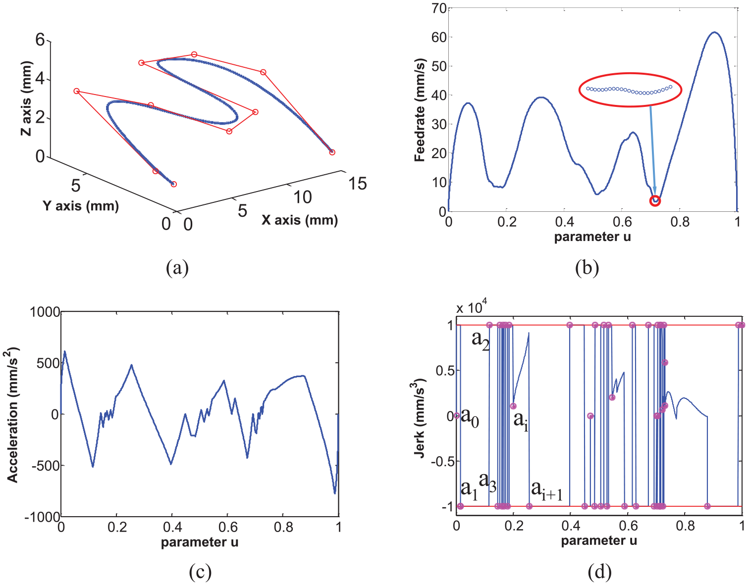
Tool path and results of scheduled federate: (a) the tool path trajectory, (b) the scheduled feedrate profile, (c) the scheduled acceleration profile, and (d) the scheduled jerk profile.
First, the feedrate profile is split according to the jerk and it is fitted in each segment. As shown in Figure 4(d), the discontinuous points of the jerk profile are a1, a2, a3,…, ai, ai + 1…. And then the parameter interval [0, 1] is constructed by subinterval [0, 0.0157], [0.0157, 0.1161], [0.1161, 0.1455], [0.1455, 0.1532] … [0.1997, 0.2563] …. The feedrate is fitted in each subinterval.
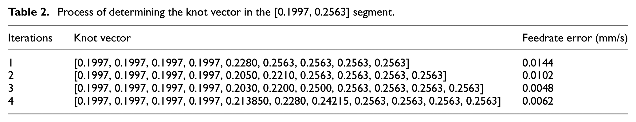
In order to explain the process of determining the knot vectors, how the knot vectors in the parameter subintervals [0, 0.0157] and [0.1997, 0.2563] (i.e. the subintervals [a0, a1], [ai, ai + 1] shown in Figure 4(d)) are distributed as shown in Table 1.
Process of determining the knot vector in the [0, 0.157] segment.
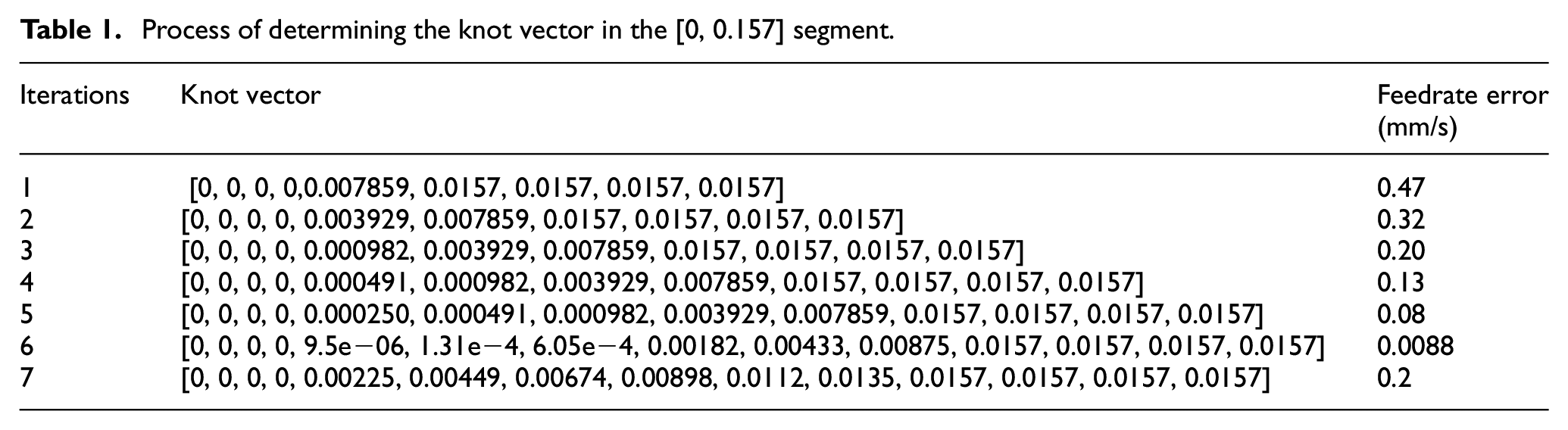
As the number of the knots required to obtain the desired accuracy is not known in advance, the approximation methods are generally used iteratively in [0, 0.0157] and [0.1997, 0.2563]. In order to ensure that the B-spline passes through the start and end control points, the multiplicity of the start and end knots is 4. The iteration process starts with nine knots which include the four start knots, four end knots, and another knot between the start and end knots. After the feedrate data points are fitted, the error between the curve and the data is checked until it satisfies the error requirements. The iterative process of determining the knot vectors for segment [0, 0.0157] and segment [0.1997, 0.2563] are listed in Tables 1 and 2, respectively.
Process of determining the knot vector in the [0.1997, 0.2563] segment.
As shown in Table 1, the feedrate in the [0, 0.0157] subinterval satisfies the feedrate error requirement after six iterations, and the knot vectors in the sixth calculation process are distributed according to the third derivative of the curve
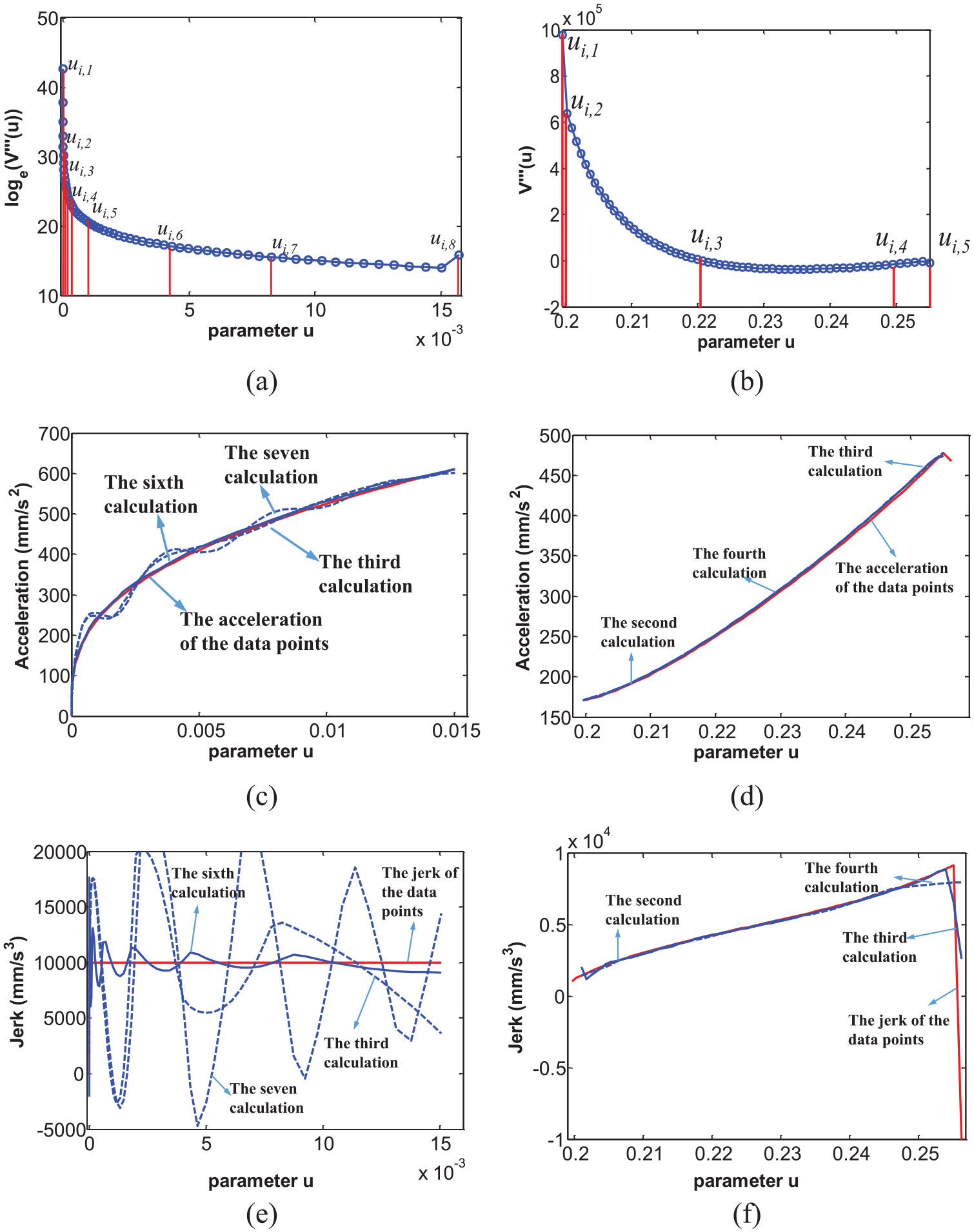
Comparison between the different iteration process and original data points: (a) third derivative in [0, 0.157] segment, (b) third derivative in [0.1997, 0.2563] segment, (c) acceleration in [0, 0.0157] segment, (d) acceleration in [0.1997, 0.2563] segment, (e) jerk in [0, 0.0157] segment, and (f) jerk in [0.1997, 0.2563] segment.
After the knot vector is selected, the control points are obtained by the least square curve approximation method. The parameters of the fitted feedrate profile curve are listed as follows:
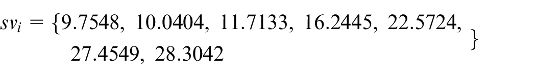
1. The parameters of the [0, 0.0157] subinterval
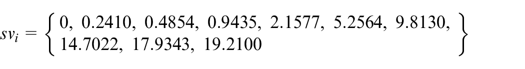
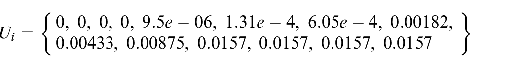

where svi, Ui and P are the control point, knot vector, and degree, respectively.
2. The parameters of the [0.1997, 0.2563] subinterval
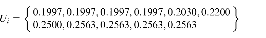

where svi, Ui and P are the control point, knot vector, and degree, respectively.
On repeating the above process, the parameters of each segment are obtained. Every segment feedrate curve needs to be composited by equations (18) and (19). The fitted feedrate profile represented by the blue curve is shown in Figure 6(a). The red curve in Figure 6(a) represents the original feedrate data. The acceleration and jerk are also calculated using numerical difference according to the fitted feedrate curve and represented by the blue curves in Figure 6(b) and (c). The original acceleration and jerk obtained by the feedrate scheduling method and represented by the red curves are also given in Figure 6(b) and (c).
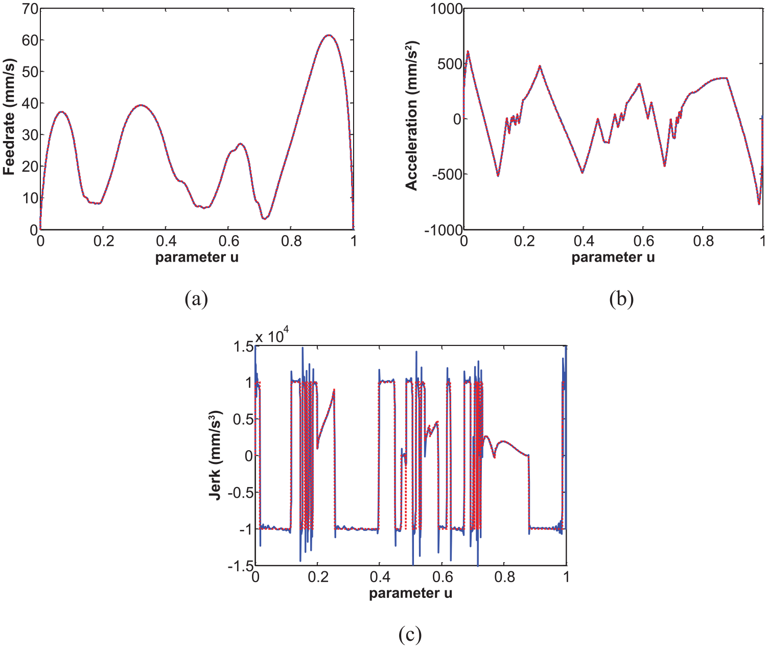
Fitted feedrate profile results: (a) the feedrate profile, (b) the acceleration profile, and (c) the jerk profile.
The proposed interpolator is validated in a software-only motion controller (A3200) developed by the Aerotech Inc. The period of the interpolation is 1 ms. In order to preliminarily verify the accuracy of the fitted feedrate profile, the drives are disconnected from the controller. The tool path and feedrate trajectory are input to the controller to command the axis. The feedrate, acceleration, and jerk that sent to drives by the interpolator are obtained from the controller, and they are shown in Figure 7. The feedrate, acceleration, and jerk of the axis are consistent with the scheduled results basically.
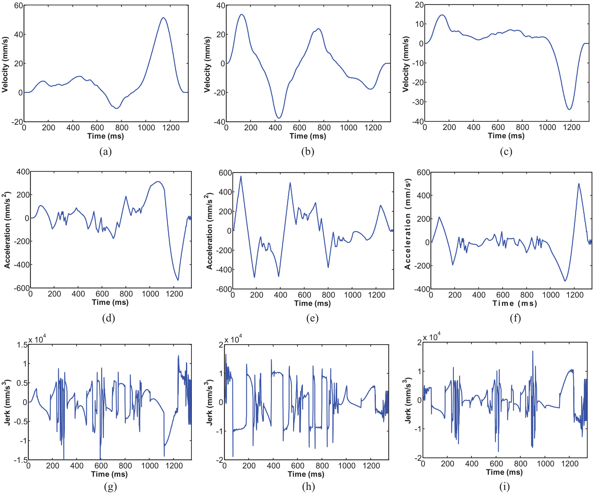
Simulation results: (a) the X-axis velocity, (b) the Y-axis velocity, (c) the Z-axis velocity, (d) the X-axis acceleration, (e) the Y-axis acceleration, (f) the Z-axis acceleration, (g) the X-axis jerk, (h) the Y-axis jerk, and (j) the Z-axis jerk.
Experiment
Case 1
In order to further validate the fitting method and the interpolation process, an experiment is carried out. The tool path is shown in Figure 8(a). The proposed interpolator is also written in the A3200 controller. The period of the interpolation is chosen as 1 ms. The platform for the experiment is shown in Figure 8(b). It is driven by two linear drives and the position is obtained by the linear encoders. The overall accuracy is ±0.5 µm.
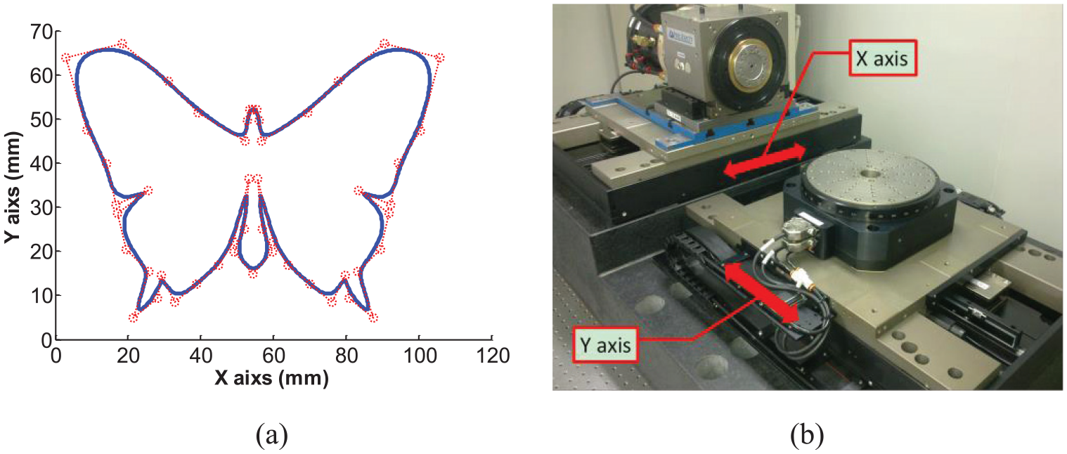
Tool path for experiment and the experiment platform: (a) the tool path for experiment and (b) the experiment platform.
The scheduled feedrate, acceleration, and jerk are shown in Figure 9(a), (c) and (e). The fitted feedrate, acceleration, and jerk are illustrated in Figure 9(b), (d) and (f), which are almost as same as the scheduled results.
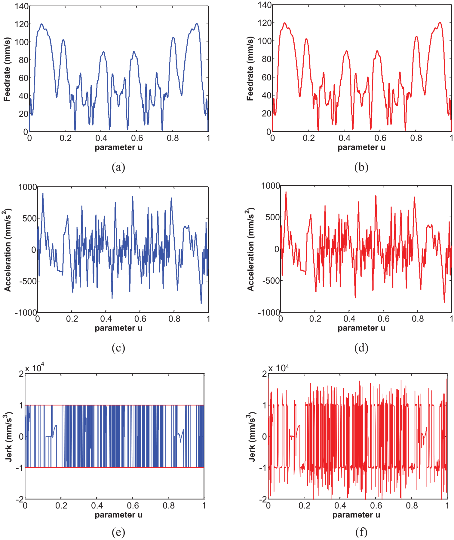
Comparison of the fitted results and the scheduled results: (a) the scheduled feedrate profile, (b) the fitted feedrate profile, (c) the scheduled acceleration profile, (d) the fitted acceleration profile, (e) the scheduled jerk profile, and (f) the fitted jerk profile.
Along with the tool path, the feedrate profile is input to the controller. The feedrates and accelerations of the X-axis and Y-axis are obtained by the linear encoders. These are shown in Figure 10. The tracking errors of the axes are also provided in Figure 10(e) and (f). As shown in Figure 10(e) and (f), the tracking errors are uniform and there are not larger tracking errors, these illustrated that the acceleration and jerk calculated by the fitted feedrate profile satisfy the error requirement.
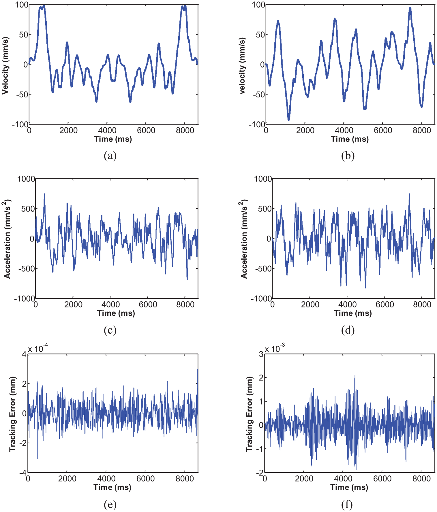
Experiment results: (a) the X-axis velocity, (b) the Y-axis velocity, (c) the X-axis acceleration, (d) the Y-axis acceleration, (e) the X-axis tracking error, and (f) the Y-axis tracking error.
Case 2
One three-dimensional (3D) tool path is carried out on a five-axis polishing machine to validate the robustness of the feedrate fitting method and the proposed interpolation method. The 3D tool path is a little modification of the butterfly and is shown in Figure 11(a). It is generated by rotating the two-dimensional (2D) butterfly tool path 45° around the X-axis. The controller of the five-axis polishing machine is also the software-only motion controller A3200. It is shown in Figure 11(b). The period of the interpolation is also chosen as 1 ms.
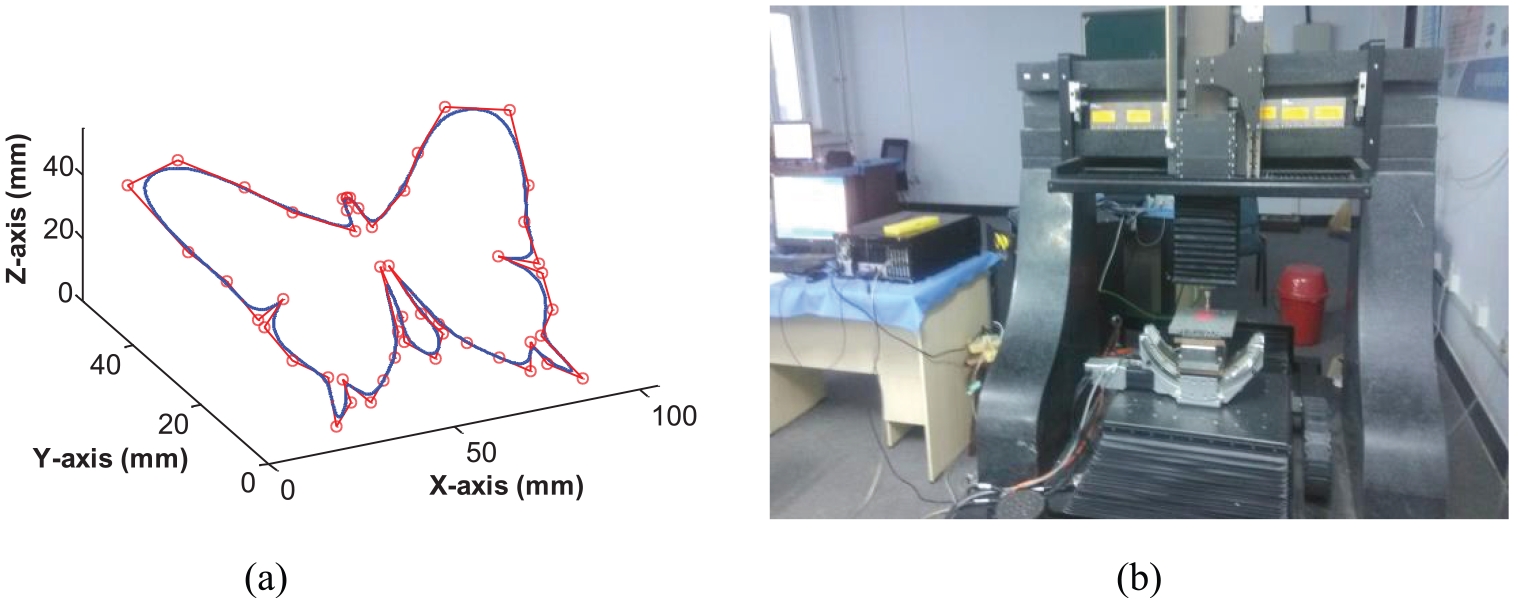
Tool path for experiment and the experiment platform: (a) the tool path for experiment and (b) the experiment platform.
The scheduled feedrate, acceleration, and jerk are shown in Figure 12(a), (c) and (e). The fitted feedrate, acceleration, and jerk are illustrated in Figure 12(b), (d) and (f), which are almost the same as the scheduled results.
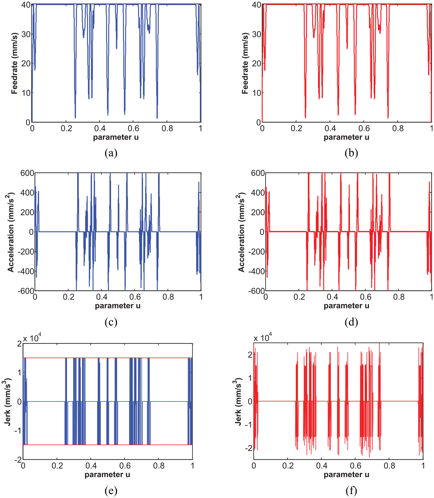
Comparison of the fitted results and the scheduled results: (a) the scheduled feedrate profile, (b) the fitted feedrate profile, (c) the scheduled acceleration profile, (d) the fitted acceleration profile, (e) the scheduled jerk profile, and (f) the fitted jerk profile.
Along with the tool path, the feedrate profile is input to the controller. The feedrates and accelerations of the X-axis, Y-axis, and Z-axis are obtained by the linear encoders. These are shown in Figure 13. The 3D tool path experiment proves that the feedrate fitting method and the proposed interpolation method are robust.
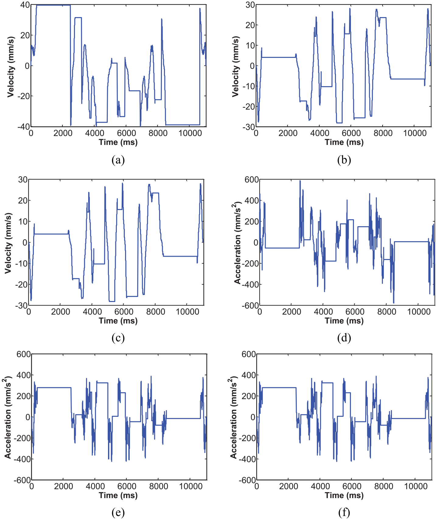
Experiment results: (a) the X-axis velocity, (b) the Y-axis velocity, (c) the Z-axis velocity, (d) the X-axis acceleration, (e) the Y-axis acceleration, and (f) the Z-axis acceleration.
Conclusion
In order to obtain an efficient and smooth machining process, the feedrate profile is scheduled by numerical calculation for the complexity of the problem. The discrete feedrate data after scheduling need to be fitted for the parametric interpolator appropriately. Although the segment feedrate profile fitting method is a common method in the profile fitting, every segment profile fitting method has their own principle to divide the original data points. In this article, the characteristic of feedrate profile and the cubic B-spline is analyzed, and the feedrate original data points are divided in the discontinuity of the jerk. In the normal profile B-spline fitting process, the knot vector is predetermined. The distribution and number of the knot vector influence the fitting error in larger. In this article, the number of the knot vector is determined by iteration, and its distribution is adjusted by the variation of the
There is always a trade-off between the computing time and precision for the interpolation process. The proposed interpolation process is separated into two parallel computing processes: the arc-length calculating process and the curve parameter calculating process. It decreases the computing load and can be executed in the controller. The novel interpolation process is both validated by the simulation and experiment.
Footnotes
Declaration of conflicting interests
The author(s) declared no potential conflicts of interest with respect to the research, authorship, and/or publication of this article.
Funding
The author(s) received the following financial support for the research, authorship, and/or publication of this article: The authors are grateful for the financial support from the National High Technology Research and Development Program (863 Program) of China (Grant No. 2012AA041304). The authors are grateful to Lecturer Yan Gu from Changchun University of Technology, who provided the equipment for the experiment of Case 2.