
Abstract
A real-time parametric interpolator based on a predictor-modification-evaluation–corrector-modification-evaluation algorithm is proposed in this article, which is utilized to efficiently calculate the reference points of transition curves. Meanwhile, the stable calculation is guaranteed by analyzing the convergence condition of the predictor-modification-evaluation–corrector-modification-evaluation algorithm. Under the convergence condition, the proposed parametric interpolator and traditional line interpolators are simultaneously implemented to interpolate a two-dimensional butterfly path, which consists of quintic Bézier transition curves and line segments. Simulation and experiments are carried out, and the results demonstrate that the proposed real-time predictor-modification-evaluation–corrector-modification-evaluation parametric interpolator achieves the highest accuracy and the light stripe on the tool path is further reduced and hardly observed. Compared with other parametric interpolators, the proposed real-time predictor-modification-evaluation–corrector-modification-evaluation parametric interpolator is capable of achieving a good balance between interpolation accuracy and interpolation efficiency.
Keywords
Introduction
In numerical control (NC) machining, line segments are widely applied to describe the complex machining graphics in light of their flexibility. 1 However, due to the discontinuities of tangency and curvature at segment junctions, the feedrate of cutting tool has to be slowed down frequently to avoid the feedrate fluctuation. To overcome the frequent acceleration and deceleration, a transition method by using a curve to transit line segments is commonly utilized. 2 With this method, a smooth tool path with curvature continuity is achieved. Then, an acceleration/deceleration (ACC/DEC) scheduling 3 and a look ahead scheme 4 are implemented simultaneously to generate the corresponding feedrate profile in real time. Based on the tool path and feedrate profile, a series of reference points are generated by the interpolator, 5 and the reference points guide the NC machining along with the path. Since the path is composed of line segments and curves, both line interpolator and parametric interpolator are involved. Generally, line interpolator is utilized to calculate the reference points on the line segment by using the analytic algorithm, so it does not cause the interpolation error. Parametric interpolator, which uses the numerical algorithm to approximate curve parameters, causes the interpolation error inevitably because there is no analytical relationship between curve length and curve parameter. Thus, the performance of the abovementioned interpolators, especially the parametric interpolator, directly affects the machining quality and efficiency.
The parametric interpolator can be divided into two categories, 6 that is, feedback method and straightforward method. By taking the feedrate command error reduction as the calculation criterion, the feedback method employs the iteration algorithm 7 to determine curve parameters, while large computation is required due to undetermined iteration number. Although some methods8,9 have been improved to reduce the number of iterations, the execution time still fluctuates greatly, which affects the machining efficiency. To deal with the problem, a fast interpolation method was proposed to achieve a high efficiency and a minimum feedrate fluctuation by accurately deducing the relation between the curve parameter and arc length. 10 However, the method was only available for cubic B-spline. The straightforward method, as indicated by its name, directly calculates the curve parameters. The typical straightforward method is Taylor’s expansion (TE) method, 11 which has the advantages of simplicity, stable execution time, and fast convergence. The first-order Taylor’s expansion (FOTE) can realize an o(T2) truncation error with a feedrate fluctuation ratio of 5.81%. 12 When the second-order Taylor’s expansion (SOTE) 13 is implemented, an o(T3) truncation error can be achieved, and the feedrate fluctuation ratio can be decreased to 0.4%. 14 However, when the curve curvature is large, the feedrate fluctuation increases because only the o(T3) truncation error is achieved. 15 To deal with this issue, a parameter-compensated algorithm was proposed, 16 which adopts a compensatory polynomial to correct the generated curve parameters. In this way, the fluctuation ratio is decreased to 0.01%. Nevertheless, the polynomial coefficients are determined by the matrix calculation, which blocks the real-time interpolation. Recently, an augmented TE method based on Heun’s algorithm was put forward to obtain a better approximation value of the curve parameter. 17 Since the convergence analysis was not analyzed, each generated parameter has to be calibrated via off-line computed knot-length pairs.
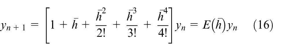
In order to decrease the feedrate fluctuation, the third-order Taylor’s expansion (TOTE) algorithm is deduced to achieve an o(T4) truncation error. The expression of the TOTE algorithm is not complicated, and the computational burden is acceptable for real-time interpolation. Meanwhile, both the effects of acceleration and jerk can be considered in the TOTE algorithm. To further achieve an o(T 5 ) truncation error for real-time interpolation, the fourth-order Runge–Kutta (FORK) algorithm, 18 rather than the fourth-order TE algorithm, is much more appropriate for simple construction, since the FORK algorithm only needs to calculate the first derivative of the curve four times in each interpolation cycle. To reduce the computation, Jahanpour and Alizadeh 19 proposed an interpolator based on the Adams–Bashforth (AB) algorithm, which needs to calculate the first derivative of the curve only once in each interpolation cycle. Actually, by combining the AB algorithm with the Adams–Moulton algorithm (ABM), the accuracy can be further improved. 20 Based on this idea, a real-time predictor-modification-evaluation–corrector-modification-evaluation (PMECME) parametric interpolator is proposed in this article, which can achieve an o(T 5 ) truncation error with certain convergence condition. Meanwhile, a quintic Bézier transition curve is introduced according to the condition, which can easily realize the stable interpolation with small calculation.
From the abovementioned analysis, it is concluded that parametric interpolator for transition curves is a key part of NC machining, but its performance is decreased due to the complexity of feedback method or the instability of straightforward method. Therefore, how to improve the stability of straightforward method is discussed here. The remainder of this article is organized as follows. In section “Principles of a quintic Bézier transition curve and a parametric interpolator,” a quintic Bézier transition curve is adopted to smooth line segments. Meanwhile, the principle of parametric interpolator is introduced briefly. In section “Parametric interpolator based on TE,” the commonly used parametric interpolator based on TE is described, and its disadvantages are discussed. In section “PMECME parametric interpolator and convergence analysis,” a parametric interpolator based on the PMECME algorithm is proposed, and the convergence condition is analyzed. The interpolation performances of different algorithms are compared in section “Simulation.” In section “Real-time interpolation experiments,” a real-time interpolation system is constructed. Meanwhile, an interpolation example is implemented to verify the effectiveness of the PMECME algorithm. The conclusions are given in section “Conclusion.”
Principles of a quintic Bézier transition curve and a parametric interpolator
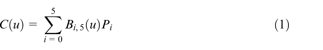
Figure 1 shows a quintic Bézier transition method between two line segments.
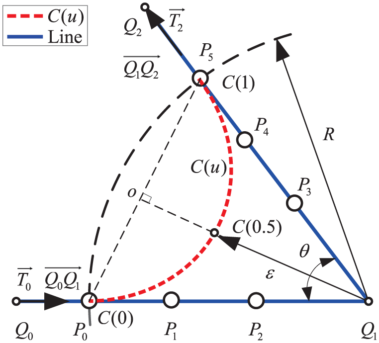
A quintic Bézier curve
To solve this issue, a quintic Bézier curve
where
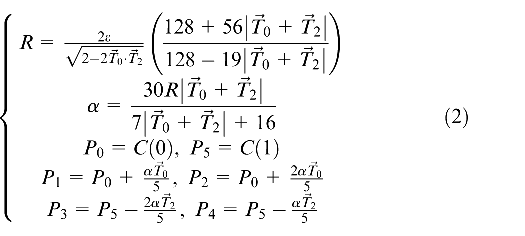
where α is a constant value. When ε or R is given, a transition curve
Generally, the parametric interpolator utilizes the numerical method to calculate the reference points, which affects interpolation accuracy and efficiency inevitably. 11 To deal with the problem, the parametric interpolator is then discussed in detail.
Parametric interpolator based on TE
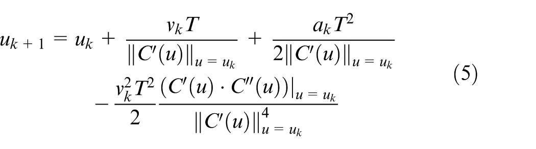
In general, TEs are widely used to establish the parametric interpolators, for example, FOTE 12 and SOTE. 13 Nevertheless, higher order TE is not commonly utilized as a parametric interpolator. The reason is as follows.
The equation of TE can be expressed as
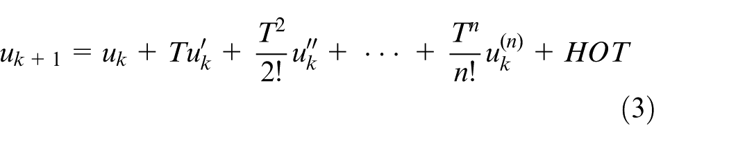
where
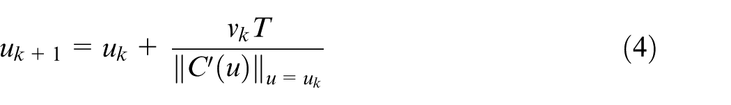
where ‖·‖ represents Euclidean norm in the three-dimensional space. Substituting equation (4) into equation (1), the reference point
where
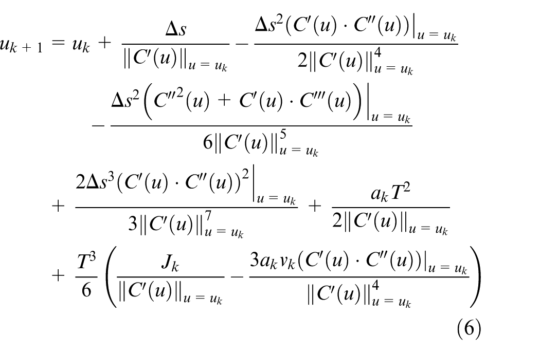
where
PMECME parametric interpolator and convergence analysis
PMECME algorithm
In this subsection, a new parametric interpolator based on the PMECME algorithm is proposed, which can achieve an
According to equation (4), a standard differential equation can be established as
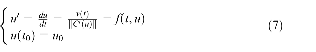
where
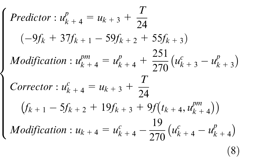
where the terms of “Predictor” and “Corrector” represent the AB four-step explicit algorithm and the Adams–Moulton (AM) three-step implicit algorithm, respectively.
PMECME algorithm can achieve o(T 5 ) truncation error, and the proof is given as follows. As shown in equation (8), the PMECME algorithm is mainly composed of four terms, which are “Predictor,”“Modification,”“Corrector,” and “Modification,” respectively. In these terms, the truncation errors of “Predictor” term and “Corrector” term are given, respectively, as 24
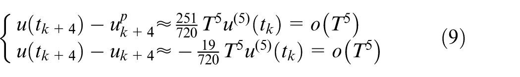
where u(tk+4) is the analytical solution at the time tk+4. According to equation (9), the difference between the errors of “Predictor” term and “Corrector” term is derived as
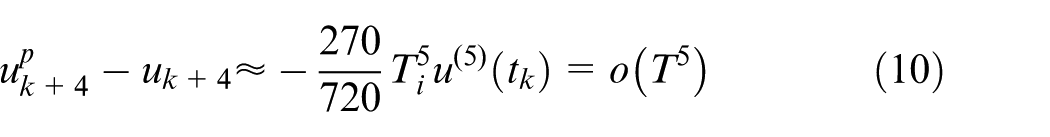
Then, substituting equation (10) into equation (9), the “modification” terms are obtained as
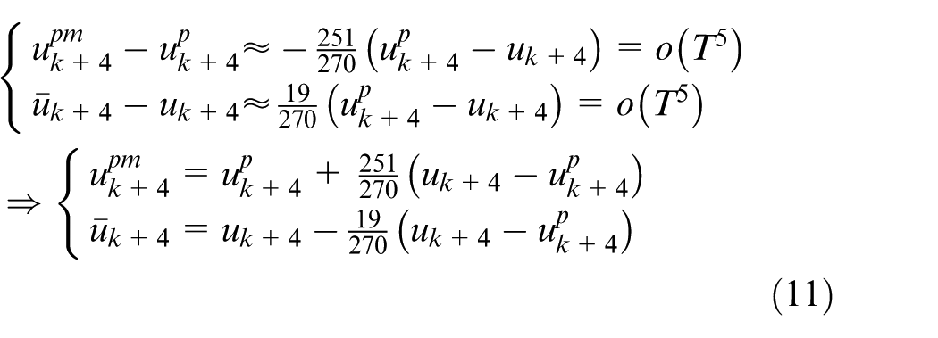
From equation (11), it can be observed that the truncation errors of “modification” are also o(T 5 ). Therefore, the PMECME algorithm can achieve o(T 5 ) truncation error.
Convergence analysis
Based on the abovementioned description, the PMECME algorithm can be used as the interpolator to compute the curve parameter in each interpolation cycle. However, the round-off error cumulates gradually in each cycle and may exceed the numerical solution eventually. Therefore, it is necessary to analyze the convergence of the PMECME algorithm. As shown in equation (8), the algorithm convergence is related to the interpolation period T. In the numerical methods, the range of T is determined by solving the first-order linear test equation 22 as follows
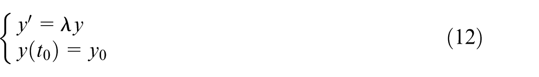
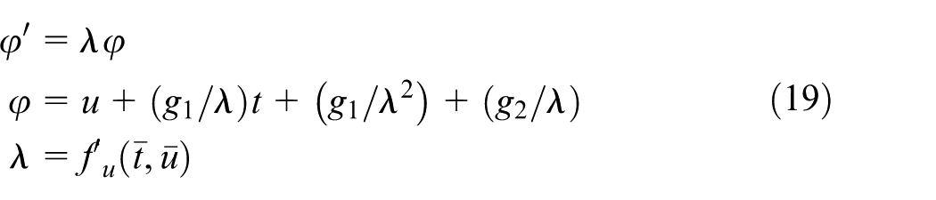
where λ is an imaginary number, and the analytical solution of equation (12) is
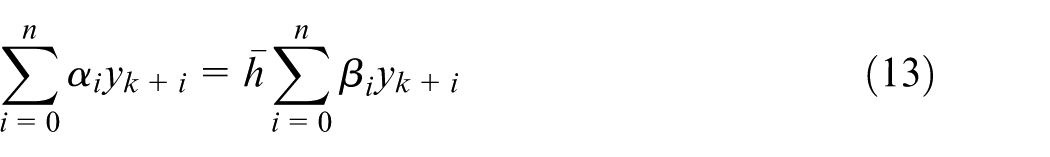
where
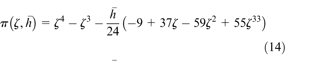
where ζ is the root of
The IASs of these algorithms.
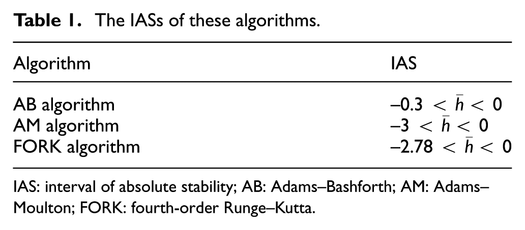
IAS: interval of absolute stability; AB: Adams–Bashforth; AM: Adams–Moulton; FORK: fourth-order Runge–Kutta.
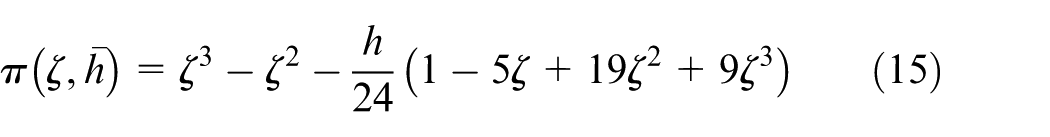
Since the initial parameters u1, u2, and u3 are acquired by the FORK algorithm, its convergence condition is also required to be analyzed. When the FORK algorithm is applied to solve equation (12), the following equation is obtained
Similarly, the FORK algorithm is stable as long as the absolute value of
From Table 1, the IAS of PMECME is determined by computing the intersection of these IASs, and it is
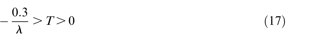
However, equation (17) only guarantees that the PMECME algorithm is stable when calculating a linear system such as equation (12), and it is not suitable for a nonlinear equation such as equation (7). Fortunately, equation (7) can be converted into a linear system approximately at the neighborhood of
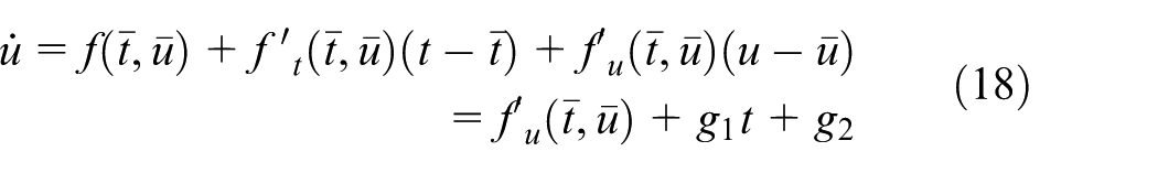
where g1 and g2 are the constant coefficients. Therefore, equation (18) can be locally linearized and transformed into a linear system as
With the abovementioned method, a linear equation is achieved. Therefore, the PMECME algorithm can be utilized to solve equation (7), and the range of T is approximated as
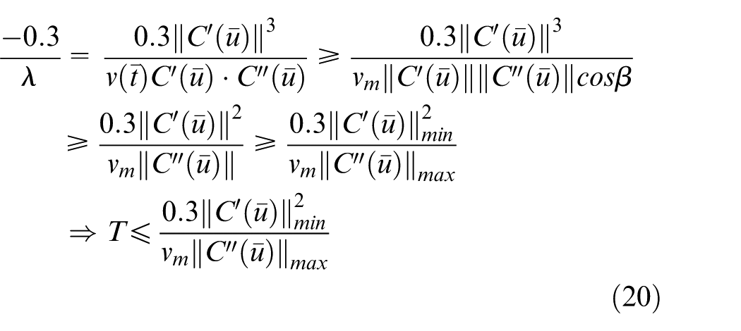
where vm indicates the maximum feedrate. Based on the abovementioned analysis, the PMECME algorithm is stable when T satisfies the convergence condition of equation (20).
Simulation
Determination of the interpolation period T
In this section, the PMECME algorithm is adopted to interpolate the quintic Bézier curve C(u). Since the property of curve
21
demonstrates that
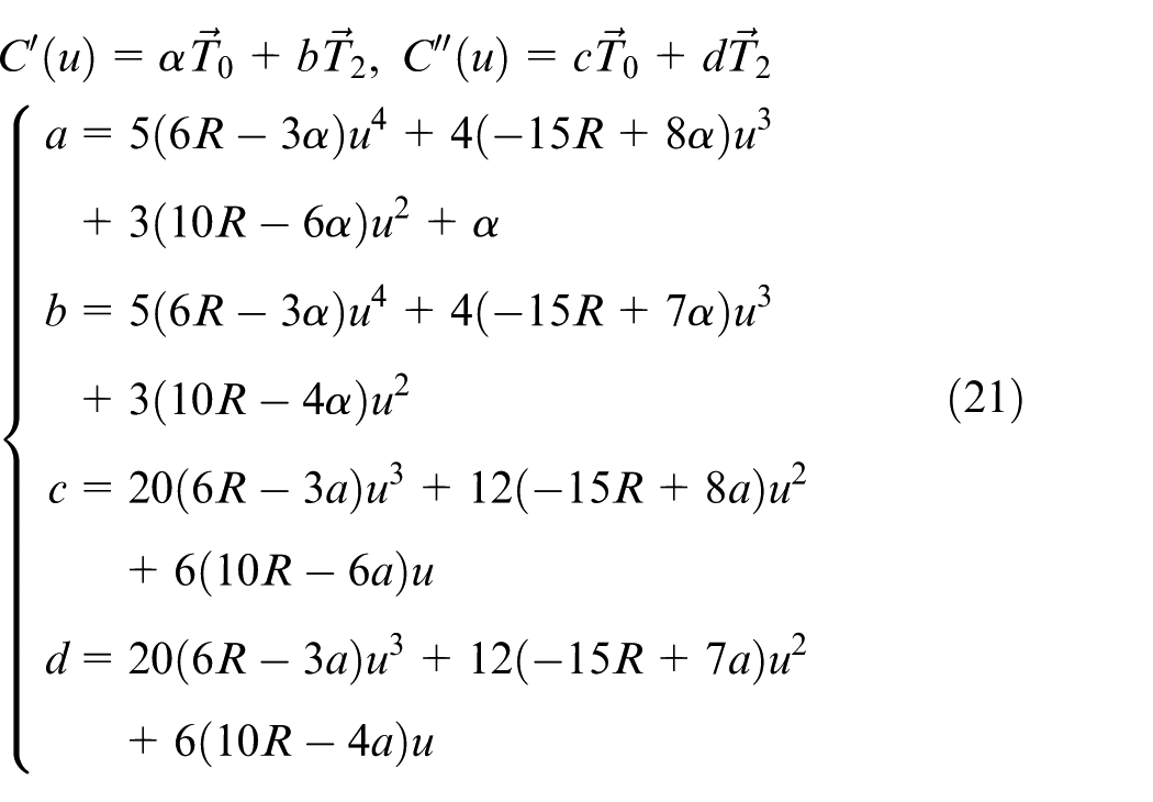
Therefore, the coefficients of

In the same way, when u is equal to 0.5, the maximum value of

When T satisfies the condition of equation (23), the stable interpolation can be guaranteed. Next, the interpolation example is given as follows.
As shown in Figure 2(a),
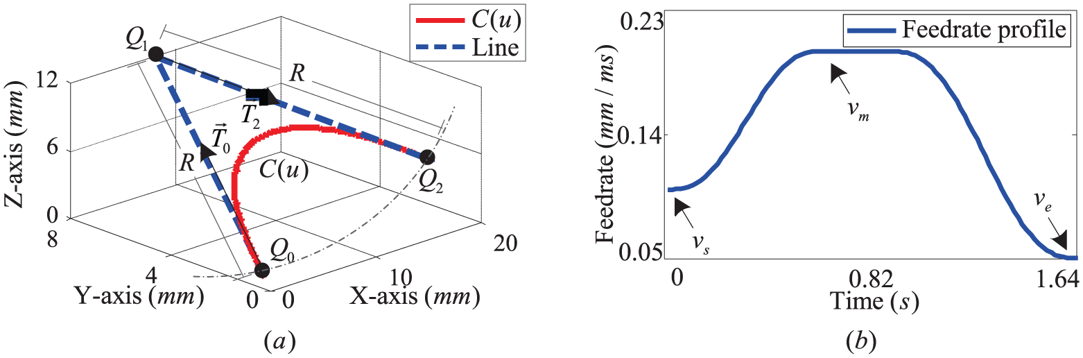
Schematic diagram of the transition Bézier curve and the generated feedrate profile: (a) a quintic Bézier transition curve and (b) the corresponding feedrate profile.
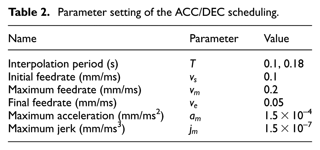
Parameter setting of the ACC/DEC scheduling.
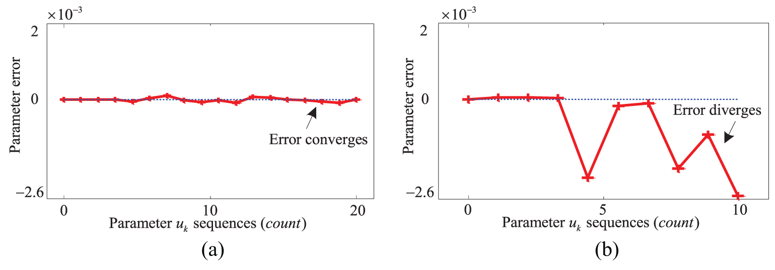
Errors of the PMECME algorithm with different interpolation periods: (a) errors of the proposed algorithm with Ti = 0.1 s and (b) errors of the proposed algorithm with Ti = 0.18 s.
Comparison of different parametric interpolators
In this section, the PMECME algorithm is introduced in the NC field, which is used as a parametric interpolator to generate reference points on the transition curve C(u) in real time.
To evaluate the performance of the PMECME algorithm, other approaches including PCI, 7 FOTE, 12 SOTE, 13 TOTE, FORK, 18 and ABM 20 algorithms are discussed here. All the algorithms are coded with Visual Studio C++ 2010 and executed in a PC configured with Intel® Core i5-3470 3.2 GHz CPU and Kingston® DDR3 1600 MHz 8G memory. The interpolation period T is chosen as 0.1 s, which is less than 0.156 s. After the interpolation, the parameter errors of these algorithms are shown in Figure 4(a) and (b), and their mean parameter errors are presented in Table 3. Meanwhile, two Win32 API functions, 28 named as “QueryPerformanceFrequency()” and “QueryPerformance Counter(),” are used to exactly record their execution time. Each algorithm is repeatedly measured 10 times, and the mean execution time is listed in Table 3.
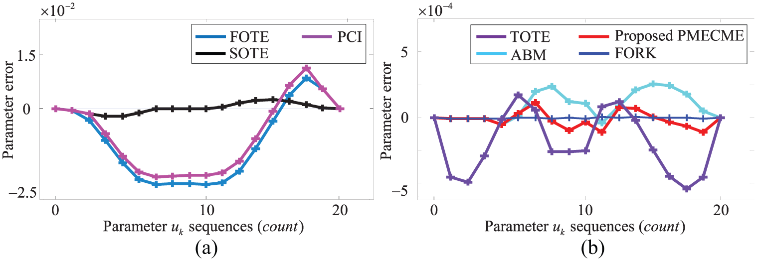
Comparison of the parameter errors generated by different algorithms: (a) errors generated by PCI, FOTE, and SOTE algorithm and (b) errors generated by TOTE, ABM, FORK, and PMECME. ABM: Adams-Bashforth-Moulton.
Statistical comparisons of the mean parameter error and the mean execution time.
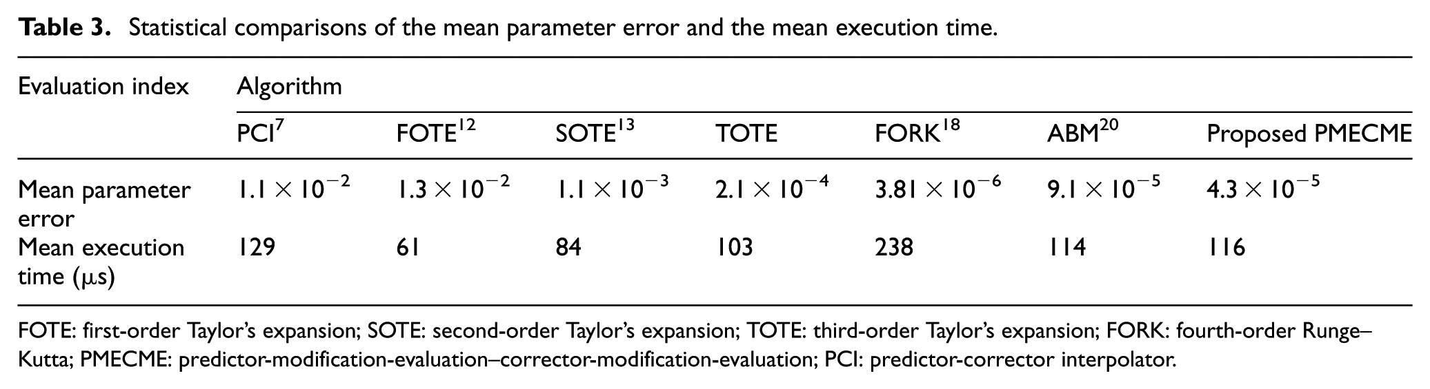
FOTE: first-order Taylor’s expansion; SOTE: second-order Taylor’s expansion; TOTE: third-order Taylor’s expansion; FORK: fourth-order Runge–Kutta; PMECME: predictor-modification-evaluation–corrector-modification-evaluation; PCI: predictor-corrector interpolator.
Real-time interpolation experiments
Real-time interpolation system construction
From Table 3, it can be observed that the current PCI iteration algorithm cannot satisfy the increasing real-time requirements of parameter error and execution time. The reason is explained as follows. As shown in Figure 5, C(uk) is a reference point and the corresponding feedrate is vk at the time tk. When the next interpolation cycle tk+1 arrives, the scheduled path is an arc
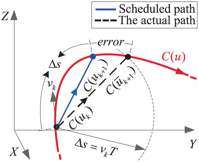
Explanation of the error generated by PCI iteration algorithm.
In this section, a real-time interpolation system is constructed, which includes a smoothing module, a look-ahead ACC/DEC scheduling module, an interpolation module, and a timer module. The relationships among them are depicted as follows. The smoothing module is responsible to smooth line segments based on the transition method as shown in section “Principles of a quintic Bézier transition curve and a parametric interpolator.” Thus, a smooth tool path including Bézier curves and line segments is generated. Then, the path is divided into several ACC/DEC schedule units (ASUs) at the midpoint of each Bézier curve. After that, the ACC/DEC scheduling 27 is implemented for each ASU to generate the corresponding feed rate profile. Since all the ASUs’ feedrate profiles could not be generated at one time due to the computational limitation of system, a look-ahead ACC/DEC scheduling module is utilized, which can generate feedrate profiles step by step (the detailed process is depicted in the next paragraph). Next, according to the generated feedrate profiles and the corresponding ASUs, reference points can be generated in real time with the cooperation of the interpolation module and the timer module. Here, the interpolation module consists of a parametric interpolator and a line interpolator. 21 In addition, the timer period is set to 10 ms based on the Win 32 multimedia timer modular (with 1 ms resolution), which aims to repeatedly activate the interrupt service routine (ISR). Meanwhile, the interpolation period T is set to 1 ms. In this way, the NC system generates 10 reference points in each ISR.
The real-time interpolation strategy in the system is given as follows. As shown in Figure 6(a), a sliding window is introduced, which can cover the maximum number of k line segments. Note that the window-sliding position is set to an integer multiple of ASU.
In the first time period (expressed as I0 in Figure 6(b)), NC system puts k line segments into the window (e.g. window 0 in Figure 6(a)). Then, the timer module activates ISR and enables other modules in ISR. First, the smoothing module smoothes these line segments and generates a smooth tool path (the solid blue lines connected with the dotted red lines in window 0). Second, the path is divided into ASUs. Then, the look-ahead ACC/DEC scheduling module obtains feedrate profiles. At last, based on ASUs and feedrate profiles, the interpolation module generates the specified number of reference points (10 points) and utilizes the points to guide the tool movement along the path.
In the next timer period, the NC system examines whether the tool has reached the window-sliding position (the position where the window 0 and windows 1 overlap). If not reached, only the interpolation module works in this ISR (the I1 in Figure 6(b)). Accordingly, the new reference points, with the same number as before, are generated and make the tool continue to move. Otherwise, the window slides forward (the window 1 in Figure 6(a)). That is to say, the line segments in front of the window-sliding position are removed from the window, and the same number of new line segments is added into the window.
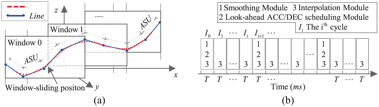
Schematic diagram of the real-time interpolation strategy: (a) the machining tool path and (b) the program of real-time interpolation.
Interpolation experiments and efficiency analysis
As shown in Figure 7(a), a NC machine with the real-time interpolation system is adopted to evaluate the computational efficiency of PMECME algorithm by imbedding the algorithm into its system. Meanwhile, other comparative algorithms including PCI, SOTE, and TOTE algorithms are also imbedded into the system, respectively.
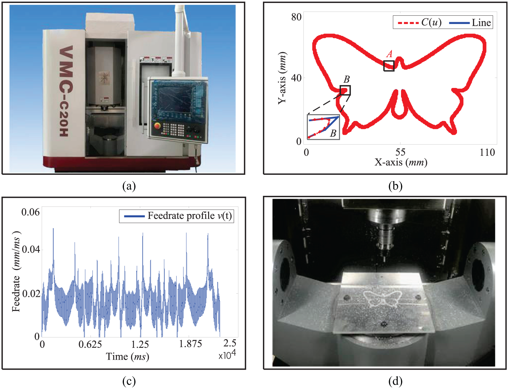
Real-time interpolation experiment of the two-dimensional butterfly pattern: (a) the NC machine used in the experiment, (b) the smooth tool path (
A butterfly graphic, which consists of 500 line segments, is used here as the test pattern for implementing the real-time interpolation task. These line segments are depicted as solid blue lines in Figure 7(b). The interpolation parameters are presented below. The timer period is set to 10 ms, and the interpolation period T is set to 1 ms. The approximation error ε is 1 mm, and the number of line segments k in each window is 5. The maximum feedrate, the maximum acceleration, and the maximum jerk are 0.05, 0.001, 2 and 0.001 mm/ms, 3 respectively. First, with the smoothing module, a smooth tool path, composed of the solid blue lines and the dotted red lines in Figure 7(b), is generated. Then, the look-ahead ACC/DEC scheduling is executed, and the generated feedrate profile of tool path is illustrated in Figure 7(c). From the figure, it can be seen that the whole interpolation task consumes 22,701 ms. After the completion of interpolation task, the tool path of each algorithm is generated and the enlarged partial view of the path is shown in Figure 8, respectively.
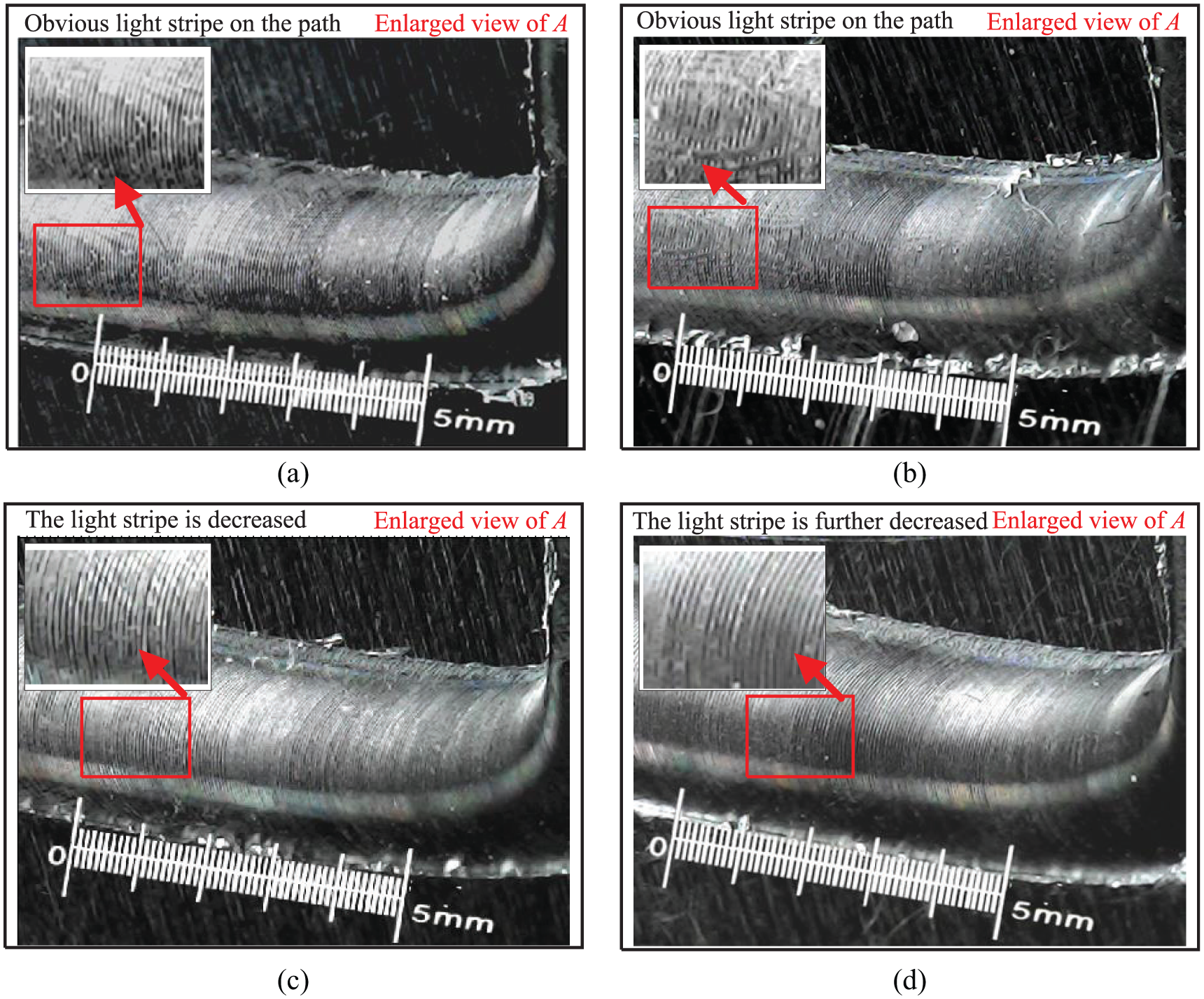
Comparison of the enlarged partial view of tool paths generated by different systems with PCI (a), SOTE (b), TOTE (c), and PMECME (d) algorithms.
The position error and execution time of each ISR are recorded and illustrated in Figures 9 and 10. Figure 9(a) shows the position error achieved by the system that uses the PCI algorithm as the parametric interpolator. The reason that causes the error has been discussed in section “Simulation.” Since the error leads to deviation of the interpolation point, there is an obvious light stripe on the tool path, which can be seen in Figure 8(a). Meanwhile, Figure 10(a) indicates the execution time of the system with the PCI algorithm. The figure indicates that this system takes the longest amount of time. Since the PCI algorithm adopts the iteration operation to calculate reference points, it is inapplicable to interpolate the transition curve in real time.
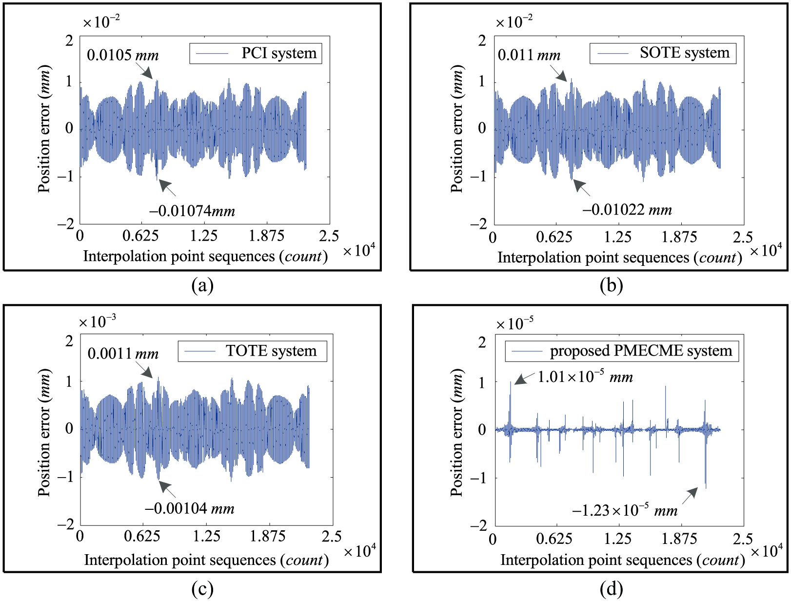
Comparison of the position errors generated by different systems with PCI (a), SOTE (b), TOTE (c), and PMECME (d) algorithms.
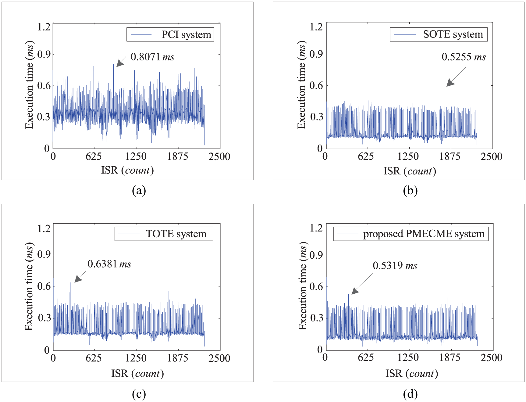
Comparison of the execution time generated by different systems with PCI (a), SOTE (b), TOTE (c), and PMECME (d) algorithms.
Figures 9(b) and 10(b) show the positron error and execution time of the system with the SOTE algorithm, respectively. Since the SOTE algorithm has the merits of flexible control and simple implementation, it is less time-consuming and has higher convergence precision than the PCI algorithm, which has been widely utilized in the NC field. However, this algorithm only achieves o(T3) truncation error, and the error may not satisfy high precision machining requirements especially when interpolating the transition curve which has the large curvature.
As shown in Figure 8(b), there is also an obvious light stripe on the tool path. To obtain o(T4) truncation error, the TOTE algorithm is deduced. Figures 9(c) and 10(c) show the position error and execution time of the system with the TOTE algorithm. As shown in the figures, this system has smaller position error than the system with the SOTE algorithm. When this system is adopted to generate the tool path, the light stripe on the path, as shown in Figure 8(c), is reduced effectively. However, the TOTE algorithm is obtained from the high-order expansion of the SOTE algorithm, so it spends longer execution time than the SOTE algorithm. Accordingly, these two systems fail to achieve good interpolation performance as shown in Table 4. When the quintic Bézier curve is specified as the transition curve, the system with the proposed PMECME algorithm, as shown in Figures 9(d) and 10(d), achieves the highest accuracy because it has the o(T 5 ) truncation error. Figure 8(d) gives the tool path generated by the system with the PMECME algorithm. In the figure, the light stripe on the tool path is further reduced and hardly observed. In addition, the convergence of the PMECME algorithm is deduced in equation (20), so the stability of the algorithm is guaranteed during the real-time interpolation. Although this system, as shown in Figure 10(d), consumes a little more time than that of the SOTE-based system, it achieves a good balance between efficiency and accuracy.
Comparison of experimental results obtained by the systems with different interpolation algorithms.
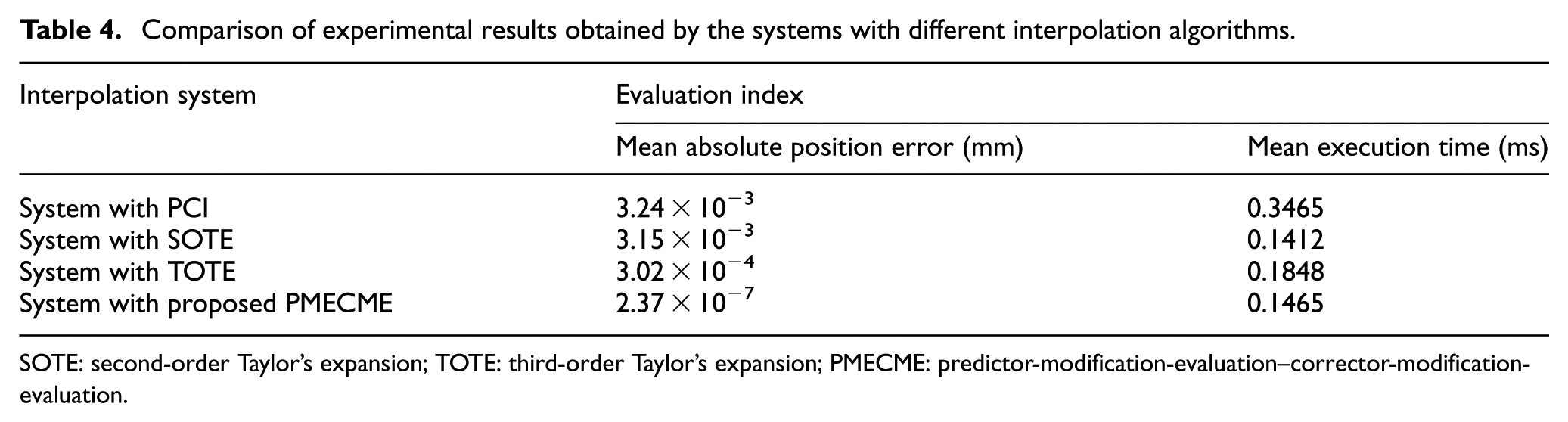
SOTE: second-order Taylor’s expansion; TOTE: third-order Taylor’s expansion; PMECME: predictor-modification-evaluation–corrector-modification-evaluation.
Conclusion
The parametric interpolator based on the TE algorithm with different orders is discussed first in this article. With the increase in the order of Taylor series, computational burden is getting more and more complicated. To deal with the issue, a parametric interpolator based on the PMECME algorithm is proposed here to achieve an o(T 5 ) truncation error, and the convergence condition is analyzed afterward. The determination of interpolation period is deduced, and different parametric interpolators are simulated to compare with each other. Simulation results show that with the PMECME algorithm, the mean execution time is decreased as well as the truncation error is further improved. Then, the proposed parametric interpolator and traditional line interpolator are simultaneously applied for real applications with a cutting tool path composing of transition curves and line segments. The performance of PMECME algorithm is evaluated through the two-dimensional butterfly interpolation experiment, and the results verify the accuracy and efficiency. The proposed PMECME algorithm achieves the highest accuracy and the light stripe on the tool path is further reduced and hardly observed.
Footnotes
Appendix 1
Declaration of conflicting interests
The author(s) declared no potential conflicts of interest with respect to the research, authorship, and/or publication of this article.
Funding
The author(s) disclosed receipt of the following financial support for the research, authorship, and/or publication of this article: This work was supported in part by National Natural Science Foundation of China (Grant No. 51805325), National Key Basic Research Program of China (Grant No. 2013CB035804), National Science and Technology Major Project (Grant No. 2015 ZX04005006), and State Key Lab of Digital Manufacturing Equipment & Technology (Grant No. DMETKF2016002).