Optimization of surface roughness in ball-end milling using teaching-learning-based optimization and response surface methodology

Abstract

Surface roughness is one of the most important requirements of the finished products in machining process. The determination of optimal cutting parameters is very important to minimize the surface roughness of a product. This article describes the development process of a surface roughness model in high-speed ball-end milling using response surface methodology based on design of experiment. Composite desirability function and teaching-learning-based optimization algorithm have been used for determining optimal cutting process parameters. The experiments have been planned and conducted using rotatable central composite design under dry condition. Mathematical model for surface roughness has been developed in terms of cutting speed, feed per tooth, axial depth of cut and radial depth of cut as the cutting process parameters. Analysis of variance has been performed for analysing the effect of cutting parameters on surface roughness. A second-order full quadratic model is used for mathematical modelling. The analysis of the results shows that the developed model is adequate enough and good to be accepted. Analysis of variance for the individual terms revealed that surface roughness is mostly affected by the cutting speed with a percentage contribution of 47.18% followed by axial depth of cut by 10.83%. The optimum values of cutting process parameters obtained through teaching-learning-based optimization are feed per tooth (f_z) = 0.06 mm, axial depth of cut (A_p) = 0.74 mm, cutting speed (V_c) = 145.8 m/min, and radial depth of cut (A_e) = 0.38 mm. The optimum value of surface roughness at the optimum parametric setting is 1.11 µm and has been validated by confirmation experiments.

Keywords

Ball-end milling composite desirability function optimization response surface methodology surface roughness teaching-learning-based optimization

Introduction

High-speed ball-end milling (HSM) is one of the modern technology, which in comparison with conventional cutting enables to increase efficiency, accuracy, and quality of product. HSM is widely used in automobile, aerospace, and die and mould-making industries, as well as in machining of propellers and turbine blades. It has been applied often for better surface finish and high productivity. It is a versatile milling process for generating complex shapes of high quality at high productivity.¹ Machining process depends on many input parameters such as feed per tooth, cutting speed, axial and radial depth of cut, tool material, and cutting tool geometry.

In machining process, product qualities are determined by their form errors and surface finishes of the finished products. Surface roughness is one of the most widely used indices of product quality. Geometric and kinematic reproduction of the cutting edge shape and trajectory results in the generation of machined surface. Since the geometry of the ball-end milling cutter is very complex, it is very important to choose appropriate cutting conditions to meet the accuracy of the finished products. Prediction of surface roughness in machining may be classified into four methods. These are as follows: (1) analytical models based on machining theory, (2) experimental investigation approach, (3) approaches based on design of experiments, and (4) artificial intelligence.² Sriyotha et al.³ developed a simulation system for the geometrical modelling of surface roughness in ball-end finish milling considering zero helix angle and vibration-free machining. The workpiece meshing was based on Z-mapping and reported that surface roughness increase with increased feed. Liu and Loftus⁴ presented the virtual simulation model for surface roughness prediction in ball nose milling process based on dynamic modelling of cutting flute considering variable helix angle and flute trajectory. However, the simulation models predict the almost similar profile of surface roughness, but generated values have large deviation from the actual milling process.

Fuh and Wu⁵ had proposed statistical model for surface quality prediction in end milling of Al alloy using the Takushi method and the response surface methodology (RSM) using the cutting factors, namely, cutting speed, feed rate, and depth of cut. RSM and Takushi methods were combined to develop the statistical model. The experiments were performed using rotatable central composite design (CCD) with half replicate. They had observed good correlation between predicted values and experimental values.

Alauddin et al.^6,7 had developed surface roughness models and determined the cutting conditions for slot milling of 190 BHN steel and Inconel 718. First- and second-order models were developed along with contour plots. Significant effect of cutting speed and axial depth of cut was observed for steel. It was reported that either increase in feed or the axial depth of cut increased the surface roughness. Same observation was found in case of slot milling of Inconel 718. Individual parametric effect was not reported. Mansour et al.⁸ successfully employed RSM to develop mathematical model of surface roughness for difficult-to-machine material EN32. Cutting parameters were cutting speed, feed rate, and axial depth of cut. First- and second-order model were developed for the speed range of 30–35 and 24–38 m/min, respectively. It was reported that the second-order model was valid on wide range of cutting speed (24–38 m/min) as compared to that of first-order model (30–35 m/min).

Lin⁹ had studied the performance analysis of TiN-coated carbide tool in face milling of stainless steel using Taguchi method. He employed three levels of each of the cutting parameters, namely, cutting speed, feed rate, and depth of cut. The author studied the effect of cutting parameters on burr height and removed volume and concluded that at low cutting speed, burr height increased linearly. It was also observed that cutting speed had a significant effect on removed volume.

An extensive work was reported by Benardos and Vosniakos² on the prediction of surface roughness in turning and milling. Various methodologies and approaches were discussed for the purpose of prediction of surface roughness. The different parameters which influence the surface roughness was presented in fishbone diagram. Vivancos et al.¹⁰ had applied design of experiment based on factorial design to study the machining parameter selection in high-speed milling of hardened steel for injection moulds. Axial depth of cut, radial depth of cut, feed per tooth, and cutting speed were the input cutting parameters. They concluded that it is possible to achieve surface roughness values in high-speed end milling close to those obtained in grinding processes. Batista et al.¹¹ studied the effect of cutting width, tool feed, and cutting directions (up or down milling) on surface roughness in high-speed ball nose milling. They had mathematically modelled cusp and scallops. The experimental results showed that the material was crushed or ploughed at the centre of the cutter. Tool feed and cutting speed were the major factors affecting surface roughness in their study. Wang and Chang¹² studied the influence of cutting conditions (dry and coolant conditions) and tool geometry on surface roughness in slot end milling of Al2014-T6 using RSM. They had reported that surface roughness in dry condition was more compared to that obtained by applying cutting fluid. In dry cutting, cutting speed, feed per tooth, concavity, and axial relief affect surface roughness significantly. Feed per tooth and concavity angle were the most dominant cutting parameters.

Ginta et al.¹³ had employed CCD to study the surface roughness models in end milling of titanium alloy. The cutting parameters were cutting speed, axial depth of cut, and feed. They reported that the developed quadratic model using CCD was able to predict the values of surface roughness very close to experimental values. Feed was the most dominant cutting parameter followed by cutting speed and axial depth of cut in their study. Ding et al.¹⁴ established empirical models for cutting forces and surface roughness considering four factors, that is, cutting speed, feed, radial depth of cut, and axial depth of cut in hard milling of AISI H13 steel using Taguchi method. They had carried out optimizations. The experiment was based on four-level orthogonal experiment. It was concluded that surface roughness increased with increase in the cutting speed for cutting speed range 100–120 m/min. Bhardwaj et al.¹⁵ studied the effect of machining parameters like feed, cutting speed, depth of cut, and insert nose radius on the average surface roughness in end milling using RSM. They had reported that the highest contribution was made by cutting speed for generation of surface roughness.

From the previous research, it was found that the most of the experimental investigations have been conducted using two-level or three-level factorial design or Taguchi design methodology to study the influence of cutting parameters on cutting forces. In two-level factorial design, only linear relationships of model can be established. Nonlinearity present in the output characteristics can be best described through three or four levels of each of the factors. The number of trial runs becomes very large in a factorial design when number of factors increases. A CCD is usually better which requires fewer experiments. In this study, experimental plans are based on CCD. The slot milling experiments have been conducted on Al2014-T6 using TiAlN-coated solid carbide ball-end milling cutter under dry condition. Average surface roughness (R_a) values have been measured and the influence of input parameters like, axial depth of cut (A_p), radial depth of cut (A_e), feed per tooth (f_z), and cutting speed (V_c) has been studied using analysis of variance (ANOVA). The regression equation correlating the above input parameters with surface roughness (output performances) has been established. The analysis was performed in MINITAB 16 software. The effect of various cutting parameters like cutting speed, axial depth of cut, feed per tooth, and radial depth of cut on surface roughness has been investigated and a nonlinear empirical relation among the input and output parameters has been established. The optimal surface roughness and cutting parameters were obtained by composite desirability function and a comparatively new evolutionary optimization technique known as teaching-learning-based optimization (TLBO).

RSM

RSM is a collection of mathematical and statistical techniques that are useful for modelling and analysis of problems in which a response of interest is influenced by several variables and the objective is to optimize the response. RSM designs help in quantifying the relationships between one or more measured responses and the input factors. Regression analysis is performed to determine the relationship between the input factors and response variables statistically. A response variable Y is postulated to be a random variable and k input variables $x_{1}, x_{2}, x_{3}, \dots, x_{k}$ are presumed to be continuous.¹⁶ Thus, it may be written as

Y = f (x_{1}, x_{2}, x_{3}, \dots, x_{k}) \pm ε

(1)

where ε measures the experimental error. The second-order polynomial in independent variable is given by

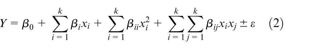
Y = β_{0} + \sum_{i = 1}^{k} β_{i} x_{i} + \sum_{i = 1}^{k} β_{ii} x_{i}^{2} + \sum_{i = 1}^{k} \sum_{j = 1}^{k} β_{ij} x_{i} x_{j} \pm ε

(2)

The least square technique is used to fit a model equation containing the regressors or input factors by minimizing the residual error and measuring sum of square deviations between the actual and estimated response model. This involves the regression coefficients of the model variables including the intercept (constant term). Once the regression equations are established, these need to be tested for statistical significance.

Optimization approaches

TLBO

TLBO is a meta-heuristic optimization algorithm based on teaching–learning process developed by Rao et al.¹⁷ This is a very efficient and accurate nature-inspired optimization technique. Rao et al.¹⁷ had applied TLBO on different mechanical design benchmark problems like design of pressure vessel, tension/compression spring, welded beam, and gear train. The effectiveness of TLBO was compared with the research available on the above-mentioned problems using different optimization techniques. They had also employed TLBO on constrained mechanical design problem available in the literature and reported that the performance of TLBO is better than the other nature-inspired optimization methods for the constrained mechanical design problems.

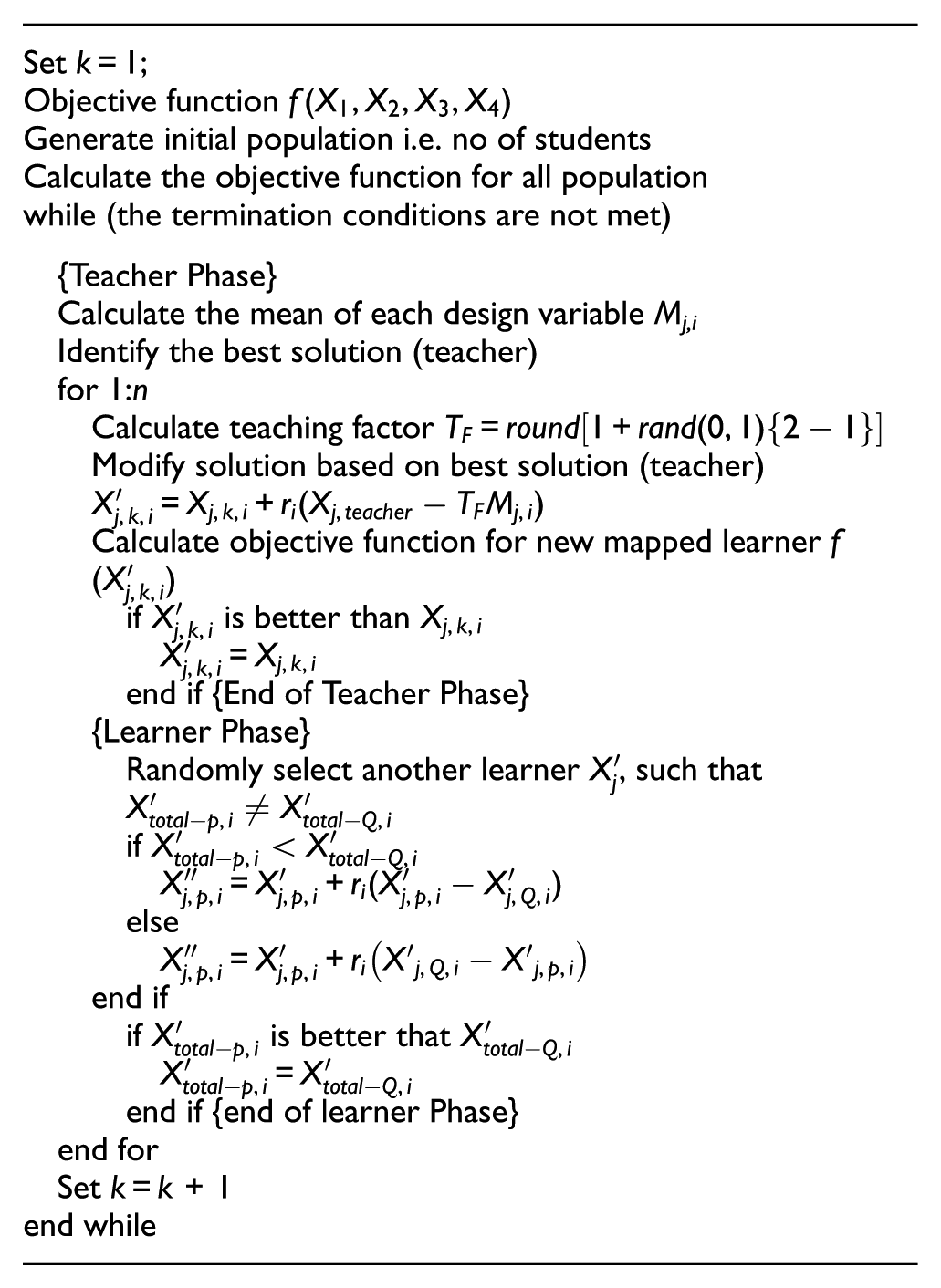
Rao et al.¹⁸ employed TLBO on nonlinear optimization problems. They had compared the TLBO and other optimization techniques like genetic algorithm (GA), particle swarm optimization (PSO), artificial bee colony (ABC), and harmony search (HS). The effectiveness of TLBO was checked on different performance criteria, namely, mean solution, success rate, average function evaluations, and convergence rate. It was reported that TLBO has better performance over other optimization techniques stated earlier. Rao and Kalyankar¹⁹ successfully applied TLBO on the examples previously attempted by various researchers for parameter optimization of different modern machining processes like ultrasonic machining, abrasive jet machining, and wire electrical discharge machining. They had also compared the results obtained by TLBO to other nature-inspired optimization techniques and reported that considerable improvement was observed in results and convergence using TLBO. Rao and Patel²⁰ had also applied TLBO for parameter optimization of a few selected casting processes like squeeze casting, continuous casting, and die casting. They had observed that results obtained from TLBO were satisfactory and require less computational efforts. Baghlani and Makiabadi²¹ employed TLBO for shape and size optimization of truss structures with dynamic frequency constraints. Considering various benchmark problems they concluded that very satisfactory results were obtained using TLBO in comparison with those of PSO, HS, and firefly algorithm (FA). TLBO is a population-based method and global optimum is obtained using the population of solutions. TLBO is based on the effect of influence of a teacher on the output of learners in a class. The algorithm mimics teaching–learning ability of teacher and learners in a class room. In TLBO the population is considered as a group of learners (students). Teacher and learners are the two vital components of the algorithm describing two basic modes of the learning, through teacher (known as teacher phase) and interacting with the other learners (known as learner phase). Thus, the algorithm is based on the teaching–learning ability of teacher and learners in a class room and is distinguished in two parts: (1) teacher phase and (2) learner phase.

Teacher phase

In a class room the teacher tries to increase the level of the knowledge of the students up to their level. But in actual practice, it is not possible (extremely difficult) to increase the knowledge level of the students to a desired level. Therefore, the teacher tries to move the mean result of the class up to some extent (close to desired level) in the specific subject taught by him or her depending on the capabilities of the class.¹⁷ Let us suppose that number of subjects also called design parameters is represented by m, and n is the number of learners (students), that is, population size. A teacher is treated as a highly knowledgeable who teaches learners for better results. Therefore, a teacher is considered as the best learner and hence tries to improve its mean results. At any particular iteration i, M_j,i is the mean result of the learners in a particular subject j. The best overall result X_{total − k teacher}, obtained in the entire population of learners considering all the subjects together can be considered as the result of best learner k_teacher. The solution is updated according to the difference between the existing mean result of each subject and the corresponding result of the teacher for each subject and can be given by

Difference_Mea n_{i, k, i} = r_{i} (X_{j, teacher} - T_{F} M_{j, i})

(3)

where X_j,teacher is the result of the best learner (i.e. teacher) in subject j, T_F is the teaching factor, and r_i is the random number varies over the range of [0, 1]. The value of T_F is decided randomly with equal probability as¹⁸

T_{F} = round [1 + rand (0, 1) \cdot {2 - 1}]

(4)

T_F is not a parameter but a heuristic step in the TLBO algorithm. The best optimal solution using TLBO can be obtained if the value of T_F is either 1 or 2 and decided randomly by the algorithm using equation (4).¹⁹ The existing solution is updated in the teacher phase using the difference mean according to the following expression shown in equation (5)

X'_{j, k, i} = X_{j, k, i} + Difference_Mea n_{j, k, i}

(5)

where $X'_{j, k, i}$ is the updated value of X_j,k,i. If $X'_{j, k, i}$ gives a better function value, then it has to be accepted. All the accepted function values at the end of the teacher phase are maintained and these values become the input to the learner phase.

Learner phase

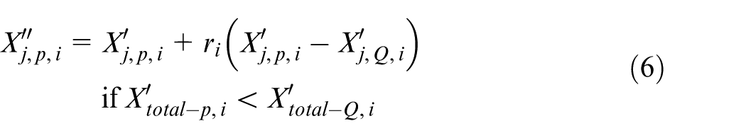
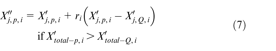
The knowledge of the learners can be increased through input from the teacher and through interaction among themselves. A learner can learn new things and enhance his or her knowledge with interacting with another learner which has more knowledge.¹⁷ For a population size of ‘n’, let us consider two learners P and Q. The learning procedure of P and Q can be obtained by the updated solution of P and Q, that is, $X'_{total - p, i} and X'_{total - Q, i}$ at the end of teacher phase under the condition that $X'_{total - p, i} \neq X'_{total - Q, i}$

{X^{″}}_{j, p, i} = {X^{'}}_{j, p, i} + r_{i} ({X^{'}}_{j, p, i} - {X^{'}}_{j, Q, i}) if {X^{'}}_{t o t a l - p, i} < {X^{'}}_{t o t a l - Q, i}

(6)

{X^{″}}_{j, p, i} = {X^{'}}_{j, p, i} + r_{i} ({X^{'}}_{j, p, i} - {X^{'}}_{j, Q, i}) if {X^{'}}_{t o t a l - p, i} > {X^{'}}_{t o t a l - Q, i}

(7)

$X_{j, p, i}^{″}$ is accepted if it gives a better functional value. All the accepted functional values obtained at the end of the learner phase restored and these values become the input to the teacher phase of the next iteration. The random values (r_i) used in equations (3), (6), and (7) may be different. Equations (6) and (7) are used for a maximization problem. The reverse is also true for the minimization problem.¹⁹ Pseudo code for TLBO for step by step demonstration is given below.

Set k = 1;

Objective function

f (X_{1}, X_{2}, X_{3}, X_{4})

Generate initial population i.e. no of students

Calculate the objective function for all population

while (the termination conditions are not met)

{Teacher Phase}

Calculate the mean of each design variable M_j,i

Identify the best solution (teacher)

for 1:n

Calculate teaching factor

T_{F} = round [1 + rand (0, 1) {2 - 1}]

Modify solution based on best solution (teacher)

X'_{j, k, i} = X_{j, k, i} + r_{i} (X_{j, teacher} - T_{F} M_{j, i})

Calculate objective function for new mapped learner f (

X'_{j, k, i}

)

X'_{j, k, i}

is better than

X_{j, k, i}

X'_{j, k, i} = X_{j, k, i}

end if {End of Teacher Phase}

{Learner Phase}

Randomly select another learner

X'_{j}

, such that

X'_{total - p, i} \neq X'_{total - Q, i}

X'_{total - p, i} < X'_{total - Q, i}

X_{j, p, i}^{″} = X'_{j, p, i} + r_{i} (X'_{j, p, i} - X'_{j, Q, i})

else

X_{j, p, i}^{″} = X'_{j, p, i} + r_{i} ({X'}_{j, Q, i} - {X'}_{j, p, i})

end if

X'_{total - p, i}

is better that

X'_{total - Q, i}

X'_{total - p, i} = X'_{total - Q, i}

end if {end of learner Phase}

end for

Set k = k + 1

end while

Response surface optimization

Response surface optimization is very useful to find out the cutting parameters (f_z, A_p, A_e, and V_c) at which the response (surface roughness) reach to the optimal value in HSM process. Optimization using RSM may be divided into three groups: (1) approach based on overlapping of contours, (2) composite desirability function, and (3) dual response system methodology.²² Composite desirability is one of the most widely used methods in industry which is based on weighted geometric mean of the individual desirability’s for the responses on a range from 0 to 1. The common approach is to find out the individual desirability index of the responses by transforming the corresponding response y_i into the individual desirability function d_i(y_i) varying over the range $0 \leq d_{i} (y_{i}) \leq 1$ using the suitable formulae as proposed by Derringer and Suich.²³ Ideal case is represented by 1 and 0 indicates the worst case, that is, one or more responses are outside the desired limits. In this approach, the inputs are target value (T_i), upper value (y_max), and lower (y_min) value of the responses. There are three forms of desirability functions: (1) the lower is the better, (2) the higher is the-better, and (3) the target is the best, depending on whether a particular response problem y_i is to be minimized, maximized, or assigned a target value. In this study, lower-is-the-better form is applied for minimizing surface roughness which may be given as

d_{i} (y_{i}) = {\begin{matrix} 1 y_{i} \leq y_{\min} \\ \frac{y_{i} - y_{\min}}{T_{i} - y_{\min}} y_{\min} \leq y_{i} \leq y_{\max}, r \geq 0 \\ 0 y_{i} \geq y_{\max} \end{matrix}

(8)

where y_min, y_max, and T_i represent lower value, upper value, and target value, respectively, of the response y_i. ‘r’ indicates the weight and its value is larger if the response is close to the target value; otherwise, it is set to the lower value. It is the most important parameter that determines the shape of the desirability function d_i(y_i). Desirability function is linear if r = 1 and convex when r > 1. If the value of r lies between 0 and 1, the shape of d_i(y_i) is concave. The individual desirability index of all the responses are then combined using the geometric mean to get the overall desirability or composite desirability D_c

D_{c} = {d_{1} {(y_{1})}^{w_{1}} * d_{2} {(y_{2})}^{w_{2}} * d_{3} {(y_{3})}^{w_{3}} * \dots * d_{m} {(y_{m})}^{w_{m}}}^{\frac{1}{W}}

(9)

where d_i (i = 1, 2, 3, …, m) is the individual desirability of the response, m_i is the weight of d_i, and W is the sum of the individual weights.

Experimental details

Milling is an intermittent multi-point cutting operation, in which each tooth is in contact with the workpiece for fraction of a spindle period. Tooth contact time varies as a function of width of cut, spindle speed, and number of flutes. Unlike turning, where chip thickness is constant, milling tool follows a trochoidal path due to the simultaneous feed and rotational motion leading to a variable chip thickness over a revolution of the cutting tool. Variation of chip thickness results in periodical change in the cutting forces acting on the tool tooth along with the entry and exit of the cutting edge. In this study, slot milling experiments have been conducted on a vertical three-axis computer numerical control (CNC) milling machine (Mikron-VCP710). Spindle speed may be varied in the range of 100–18,000 r/min and maximum work feed recommended for the vertical milling machine is 15 m/min. The maximum traverses in X, Y, and Z directions are 700, 500, and 500 mm, respectively, and maximum rapid traverse is 30 m/min. Two flute solid carbide ball-end milling cutter of diameter 10 mm (Sandvik coromant CoroMill Plura, R216.42-10030-Al10G 1620), helix angle 30°, and rake angle 4° with monolayer of TiAlN (by physical vapour deposition method) coating has been used. This type of coating increases wear resistance and may reduce cutting forces and temperatures at the tool edge. Altogether, the heat generated in the machining zone is less and that is why the use of cutting fluid has been avoided and thus the HSM milling experiments have been conducted in dry environment. However, in high-speed machining of aluminium alloys, high cutting speeds, centrifugal forces, and pressure reduce the effectiveness of the cutting fluid.²⁴ The feed direction is Y-axis and cross feed direction is along X-axis. The slot milling performance tests have been performed on aluminium alloy Al2014-T6 which covers a wide variety of applications in automotive and aerospace industries. The standard chemical composition, mechanical and thermal properties of Al2014-T6 supplied by the manufacturer (Bharat Aerospace Metals, Mumbai, India) is shown in Tables 1 and 2, respectively. The dimension of workpiece is 160 mm × 100 mm × 100 mm.

Table 1.

Chemical composition (wt%) of Al2014-T6 alloy.

Element	Cu	Si	Mg	Fe	Zn	Ti	Mn	Cr	Al
Amount (%)	3.9	0.7	0.8	0.7	0.15	0.2	0.4	0.1	Balance

Table 2.

Mechanical and thermal properties of Al2014-T6 alloy.

Tensile strength (MPa)	483	Fatigue strength (MPa)	124
Yield strength (MPa)	414	Density (g/cc)	2.8
Elongation (%)	13	Melting point (°C)	638
Hardness (HB)	135	Thermal conductivity (W/m K)	154
Shear strength (MPa)	240	Specific heat capacity (J/g °C)	0.88

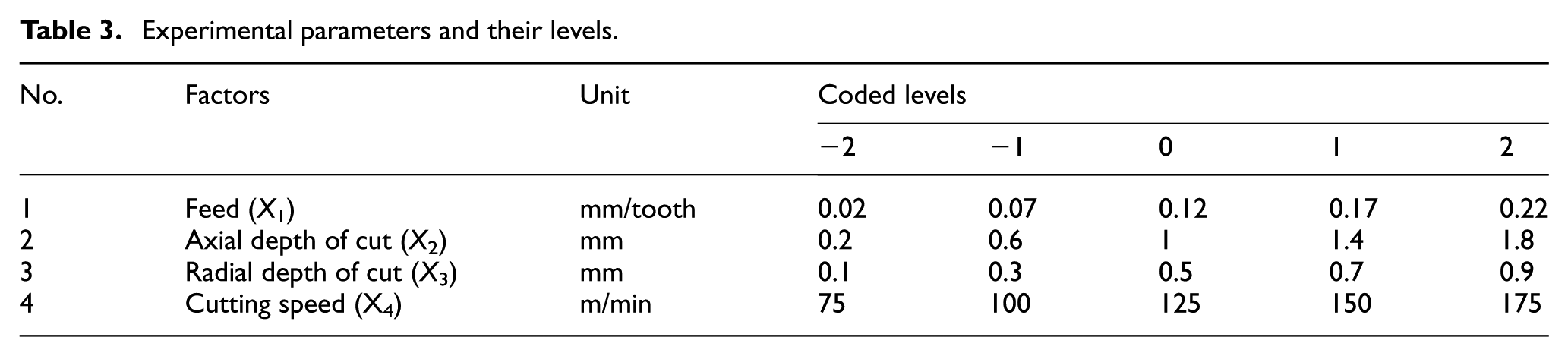
Influence of four machining parameters on the surface roughness, namely, feed per tooth (f_z), axial depth of cut (A_p), radial depth of cut (A_e), and cutting speed (V_c) have been studied. These parameters have been chosen as independent input variables. The coded values of the parameters are shown in the Table 3. A rotatable CCD has been used as a standard RSM design to study the slot milling process. The model consists of 16 cube points, 7 central points, and 8 axial points. The upper and lower limits of the factors were coded as −2 and 2, respectively. The coded values of intermediate levels can be obtained from equation (10).

X_{i} = 2 \frac{[2 X - (X_{\max} + X_{\min})]}{X_{\max} - X_{\min}}

(10)

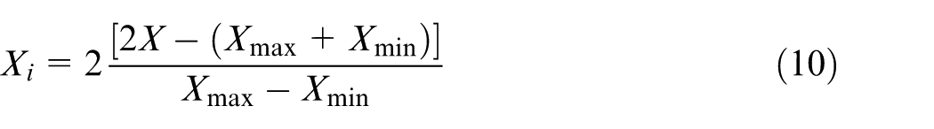
where X_i is the required coded value of the variable X. X is any value of variable from X_min to X_max. The response variable is arithmetic average surface roughness (R_a). The experimental design matrix consists of 31 runs. The experimental setup is shown in Figure 1.

Table 3.

Experimental parameters and their levels.

No.	Factors	Unit	Coded levels
No.	Factors	Unit	−2	−1	0	1	2
1	Feed (X₁)	mm/tooth	0.02	0.07	0.12	0.17	0.22
2	Axial depth of cut (X₂)	mm	0.2	0.6	1	1.4	1.8
3	Radial depth of cut (X₃)	mm	0.1	0.3	0.5	0.7	0.9
4	Cutting speed (X₄)	m/min	75	100	125	150	175

Figure 1.

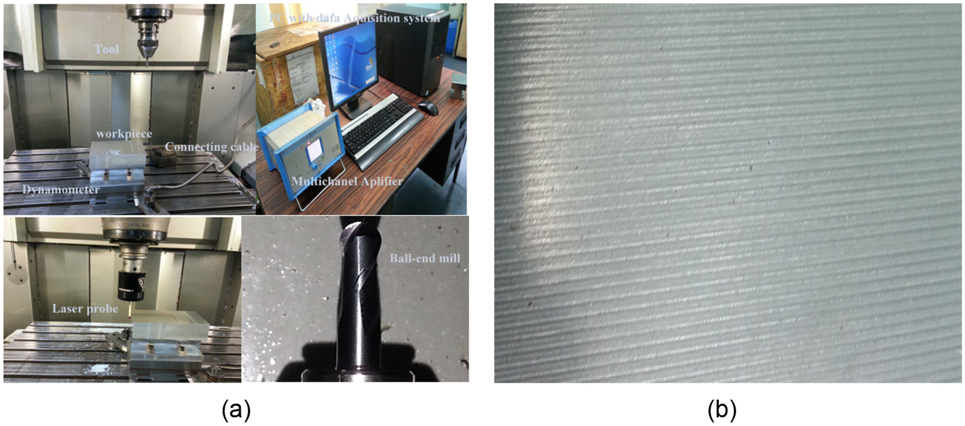
(a) Experimental setup and (b) machined surface: f_z = 0.17 mm/tooth, A_p = 0.6 mm, A_e = 0.3 mm, and V_c = 150 mm.

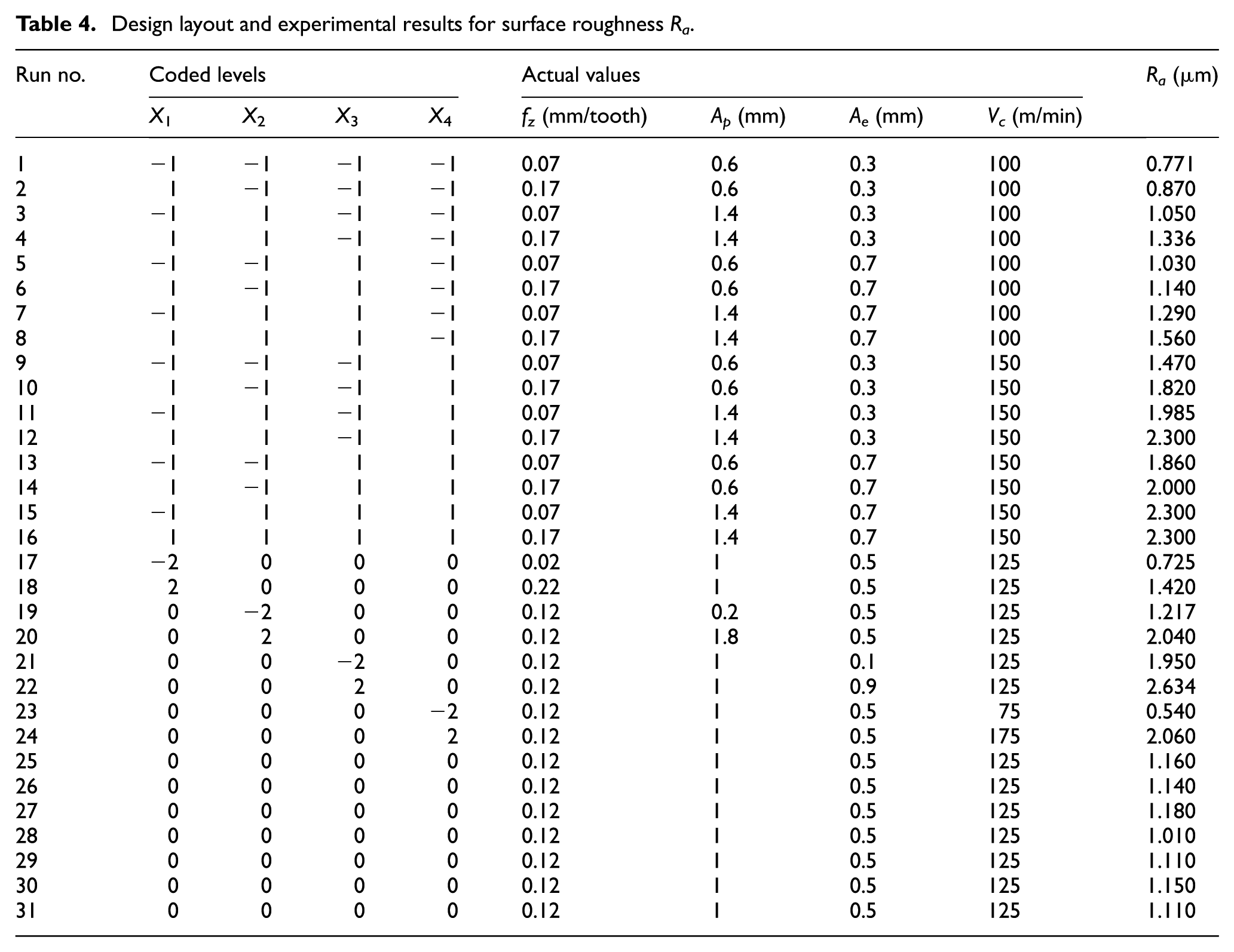
An I-shaped workpiece was prepared using flat end milling cutter. A non-contact laser probe was used to ensure the flatness of the newly machined surface. A set of 31 experiments were performed in two steps on the I-shaped Al2014-T6 workpiece of length 160 mm and width 100 mm. In the first step, the whole length of the workpiece was divided into 16 parts evenly. After collecting the desired data, the workpiece was again prepared for machining in similar way as stated above. In the second step, 15 experiments were performed. The whole experiment has been performed in standard order as shown in Table 4. After machining, the surface roughness has been measured for all the experimental runs using a surface texture measuring system (Model: Talysurf 6, Make: Taylor Hobson, UK) as per ISO standard, 4287-1997. The sampling length and traversing length were 0.25 and 25 mm, respectively. Thus, the arithmetic average roughness (R_a) data have been collected by moving stylus tip in a straight line along the slot milled grooves. The response value R_a has been measured at three different spots randomly on the machined surface and the average of the three surface roughness values has been considered as the response variable to analyse the effect of different cutting parameters. The experimental design matrix and arithmetic average surface roughness data (R_a) are shown in Table 4.

Table 4.

Design layout and experimental results for surface roughness R_a.

Run no.	Coded levels				Actual values				R_a (µm)
Run no.	X ₁	X ₂	X ₃	X ₄	f_z (mm/tooth)	A_p (mm)	A_e (mm)	V_c (m/min)	R_a (µm)
1	−1	−1	−1	−1	0.07	0.6	0.3	100	0.771
2	1	−1	−1	−1	0.17	0.6	0.3	100	0.870
3	−1	1	−1	−1	0.07	1.4	0.3	100	1.050
4	1	1	−1	−1	0.17	1.4	0.3	100	1.336
5	−1	−1	1	−1	0.07	0.6	0.7	100	1.030
6	1	−1	1	−1	0.17	0.6	0.7	100	1.140
7	−1	1	1	−1	0.07	1.4	0.7	100	1.290
8	1	1	1	−1	0.17	1.4	0.7	100	1.560
9	−1	−1	−1	1	0.07	0.6	0.3	150	1.470
10	1	−1	−1	1	0.17	0.6	0.3	150	1.820
11	−1	1	−1	1	0.07	1.4	0.3	150	1.985
12	1	1	−1	1	0.17	1.4	0.3	150	2.300
13	−1	−1	1	1	0.07	0.6	0.7	150	1.860
14	1	−1	1	1	0.17	0.6	0.7	150	2.000
15	−1	1	1	1	0.07	1.4	0.7	150	2.300
16	1	1	1	1	0.17	1.4	0.7	150	2.300
17	−2	0	0	0	0.02	1	0.5	125	0.725
18	2	0	0	0	0.22	1	0.5	125	1.420
19	0	−2	0	0	0.12	0.2	0.5	125	1.217
20	0	2	0	0	0.12	1.8	0.5	125	2.040
21	0	0	−2	0	0.12	1	0.1	125	1.950
22	0	0	2	0	0.12	1	0.9	125	2.634
23	0	0	0	−2	0.12	1	0.5	75	0.540
24	0	0	0	2	0.12	1	0.5	175	2.060
25	0	0	0	0	0.12	1	0.5	125	1.160
26	0	0	0	0	0.12	1	0.5	125	1.140
27	0	0	0	0	0.12	1	0.5	125	1.180
28	0	0	0	0	0.12	1	0.5	125	1.010
29	0	0	0	0	0.12	1	0.5	125	1.110
30	0	0	0	0	0.12	1	0.5	125	1.150
31	0	0	0	0	0.12	1	0.5	125	1.110

Results and discussion

As shown in Table 4, the experimental results have been analysed using a statistical software MINITAB 16. A mathematical model has been established among the input parameters and the surface roughness as per the foregoing discussion. The level of confidence has been considered to be 95%.

ANOVA and mathematical model development

ANOVA is very useful in drawing inferences based on statistical analysis. Test of significance for regression model and individual model coefficients are commonly obtained by the ANOVA. The terms which do not affect the model significantly may be eliminated using backward elimination, forward addition, or stepwise elimination method. Thus, significant terms are identified by conducting significance test for individual terms of the model and are shown in Table 5. It has been observed that all the linear terms are significant and all the interaction terms are insignificant. Among the squared terms, all the terms have been found to be significant except X₁*X₁. In this study, insignificant terms have been eliminated using backward elimination process. Thus, ANOVA of the model parameters is further carried out after backward elimination and has been presented in Table 6.

Table 5.

Analysis of variance for surface roughness R_a.

Sources	DoF	Seq SS	F value	p value	Significance <0.05
Model	14	8.76041	83.47	0.000	Significant
X ₁	1	0.36507	48.7	0.000	Significant
X ₂	1	0.96240	128.38	0.000	Significant
X ₃	1	0.43902	58.56	0.000	Significant
X ₄	1	4.19003	558.92	0.000	Significant
X ₁*X₁	1	0.08545	0.7	0.416	Insignificant
X ₂*X₂	1	0.25407	60.05	0.000	Significant
X ₃*X₃	1	2.37800	323.79	0.000	Significant
X ₄*X₄	1	0.05373	7.17	0.000	Significant
X ₁*X₂	1	0.00185	0.25	0.626	Insignificant
X ₁*X₃	1	0.01756	2.34	0.145	Significant
X ₁*X₄	1	0.00010	0.01	0.909	Insignificant
X ₂*X₃	1	0.00640	0.85	0.369	Insignificant
X ₂*X₄	1	0.00601	0.8	0.369	Insignificant
X ₃*X₄	1	0.00073	0.1	0.759	Insignificant
Residual error	16	0.11995	−	−	−
Lack-of-fit	10	0.10120	3.24	0.082	Insignificant
Pure error	6	0.01874	−	−	−
Total	30	8.88036	−	−	−

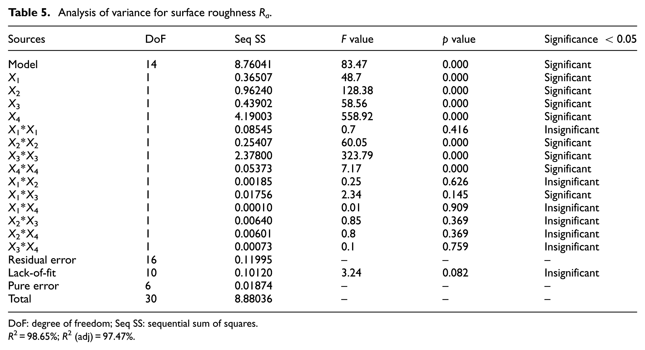
DoF: degree of freedom; Seq SS: sequential sum of squares.

R ² = 98.65%; R² (adj) = 97.47%.

Table 6.

Analysis of variance for surface roughness R_a (backward elimination).

Sources	DoF	Seq SS	F value	p value	PC
Model	7	8.72	181.60	0.000	98.19
X ₁	1	0.365	53.20	0.000	4.11
X ₂	1	0.962	140.26	0.000	10.83
X ₃	1	0.439	63.98	0.000	4.94
X ₄	1	4.190	610.64	0.000	47.18
X ₂*X₂	1	0.278	67.89	0.000	3.13
X ₃*X₃	1	2.429	361.34	0.000	27.35
X ₄*X₄	1	0.058	8.46	0.008	0.65
Residual error	23	0.157	−	−	1.76
Lack-of-Fit	17	0.139	2.62	0.119	1.56
Pure error	6	0.018	−	−	0.20
Total	30	8.88	−	−	−

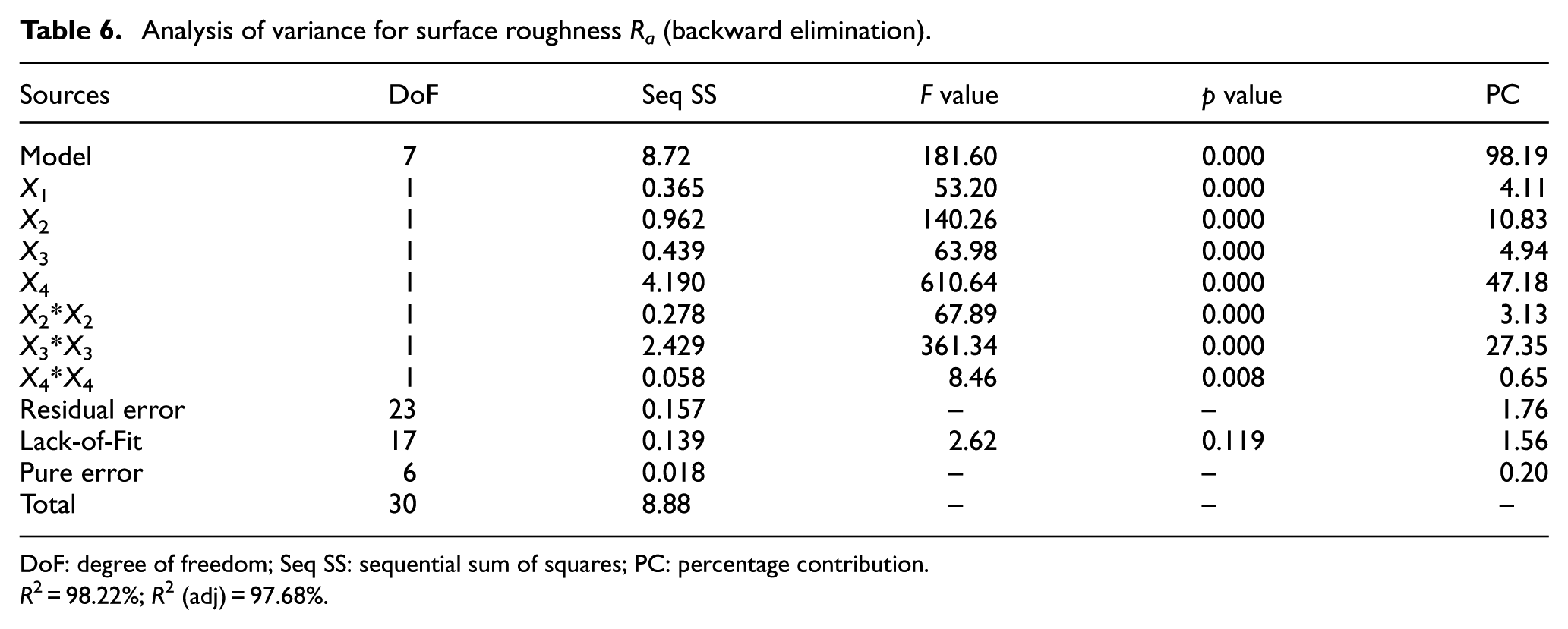
DoF: degree of freedom; Seq SS: sequential sum of squares; PC: percentage contribution.

R ² = 98.22%; R² (adj) = 97.68%.

Adequacy test for the developed model

Table 6 reveals that the second-order regression model for R_a is significant (p = 0.00). Lack-of-fit is insignificant (p = 0.119) which is desirable. R² is one of the most important statistics which is a measure of the amount of reduction in the variability of response obtained using the regressor variables in the model. Always a higher value of R² is desirable (closer to 1). A large value of R² does not imply that the regression model is good. The value of R² increases when a variable is added to the model. Therefore, adjusted R² is preferred. It often decreases if unnecessary terms are added.¹⁶ The presence of insignificant terms in model can be also identified with the difference between R² and R² (adj). Larger is the difference indicates that insignificant terms have been included in the model. From Table 6, it can be seen that the difference between R² and R² (adj) of the reduced model is very small (0.0054). The obtained R² (adj) value (0.9768) is very close to unity which shows a very good correlation between experimental and predicted results.

F test has been performed to check the adequacy of the developed model. The model is considered to be adequate when the F value for lack-of-fit of the developed model is less than the standard tabulated F value (4.06) at 95% confidence level. After eliminating the insignificant terms through backward elimination, the F value of lack-of-fit has become 2.62 (Table 6), which indicates that the model is still adequate.

Analysis of the parametric influences on the response

Percentage contribution (PC) of each significant terms of the reduced model is shown in Table 6. It is found that cutting speed is the most significant parameter accounting for 47.18% in linear part. The PC of feed per tooth, axial depth of cut, and radial depth of cut is 4.11%, 10.93%, and 4.92%, respectively. The interaction terms are found to be insignificant. It is further observed that cutting speed is the dominant cutting parameter among all the four parameters which influence surface roughness very much in HSM milling.

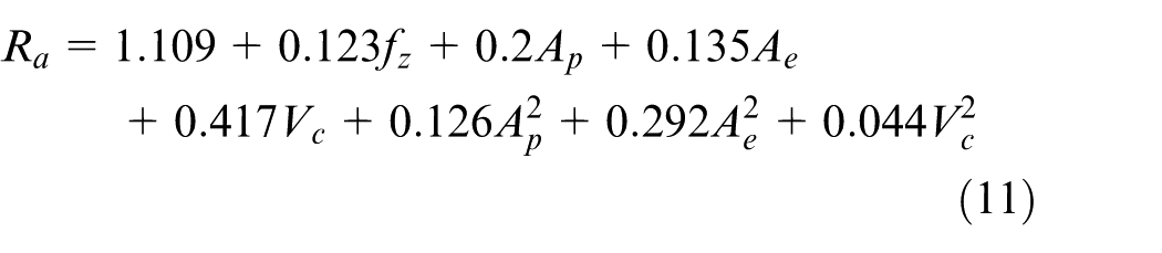
Surface plots for the surface roughness are shown in the Figure 2. Roughness has curvilinear profile in accordance with the fitted quadratic model. Surface roughness increases with the increase in feed. From the surface plot profile shown in the Figure 2(a), (b), and (d), it may be observed that the surface roughness first decreases and then increases, with increase in radial depth of cut. Surface roughness decreases when radial depth of cut increased from 0.1 to 0.5 mm. The increasing trend of surface roughness is observed when radial depth of cut increases from 0.5 to 0.9 mm. Surface roughness also increases with increase in feed per tooth for all the combinations of the cutting parameters as shown in Figure 2(d)–(f). At lower axial depth of cut, the surface roughness increases with the increase in radial depth of cut. It is observed that the change in surface roughness is small by increasing feed per tooth as compared to the radial depth of cut. Therefore, surface roughness may be decreased by decreasing radial depth of cut. The regression equations for the arithmetic average surface roughness in terms of coded level are as follows

R_{a} = 1.109 + 0.123 f_{z} + 0.2 A_{p} + 0.135 A_{e} + 0.417 V_{c} + 0.126 A_{p}^{2} + 0.292 A_{e}^{2} + 0.044 V_{c}^{2}

(11)

Figure 2.

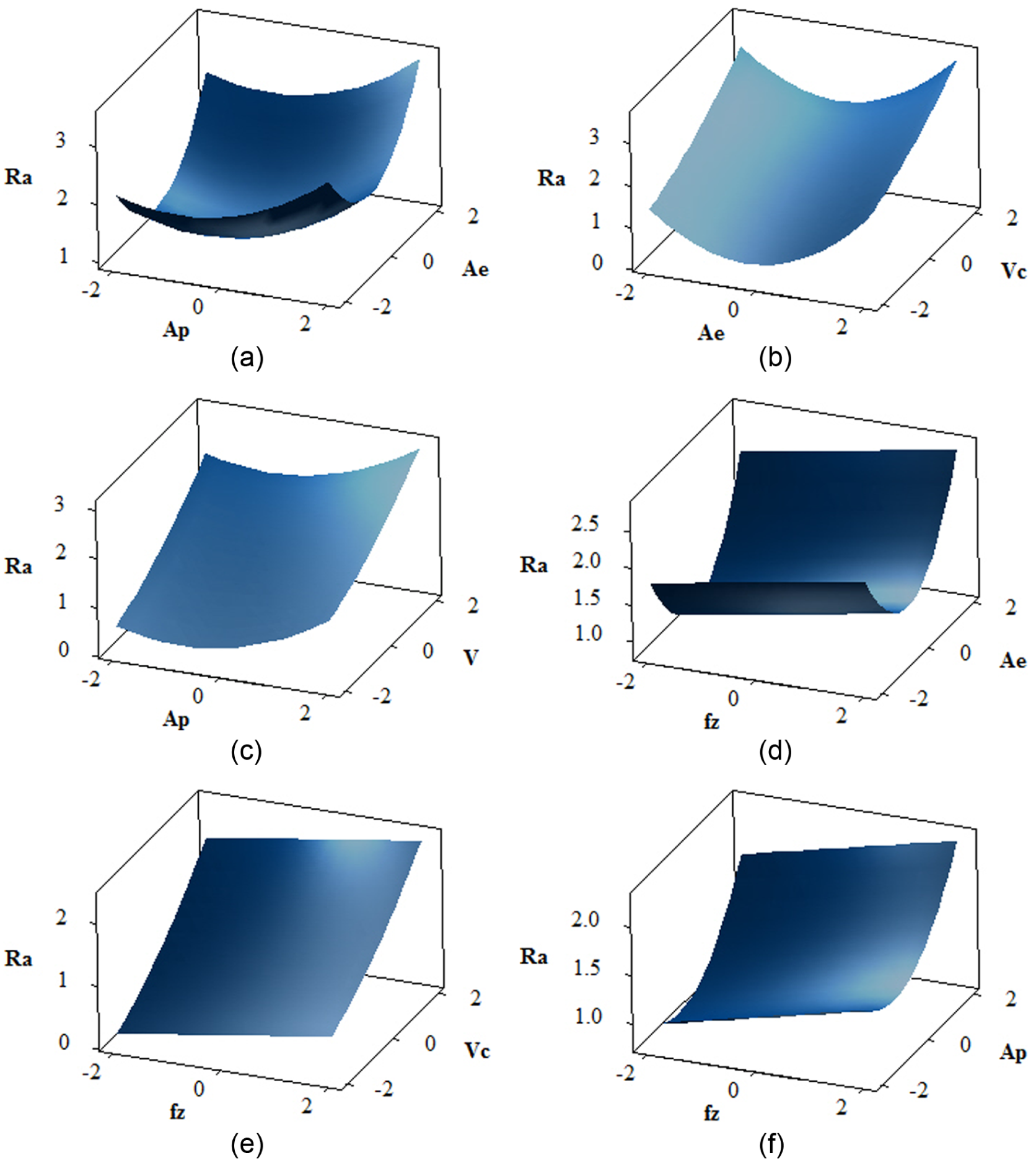
Response surface plots for surface roughness (R_a) µm: (a) R_a as a function of axial and radial depth of cut, (b) R_a as a function radial depth of cut and cutting speed, (c) R_a as a function of axial depth of cut and cutting speed, (d) R_a as a function of feed per tooth and radial depth of cut, (e) R_a as a function of feed per tooth and cutting speed, and (f) R_a as a function of feed per tooth and axial depth of cut.

Optimization of surface roughness

In this article, minimization of surface roughness has been formulated. The empirical equation of surface roughness has been developed through RSM as discussed previously. The adequacy and variability of the developed model have been tested and found that the developed model is adequate and can be used for the further processing.

Optimization using RSM

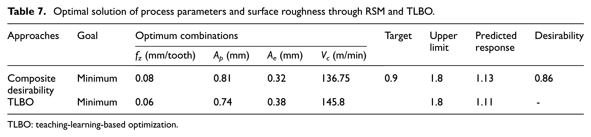
In this article, the objective (goal) is to minimize surface roughness in a desired range of 0.9–1.8 µm. The optimization results for surface roughness have been shown in Figure 3. In Figure 3, columns represent cutting parameters, while a row corresponds to response. Variation of response is indicated by each cell of the plot with change of a parameter keeping other parameters fixed. The current parameter settings are indicated at middle row of the top of the column and can change with the parameter settings interactively. The response (surface roughness, R_a), goal for the response minimization, predicted values of responses at the current parameter settings with individual desirability score is indicated at each row in left column. The optimum results for surface roughness (R_a) using RSM optimization is shown in Table 7. The optimum cutting parameters in coded unit are found to be feed per tooth of at level −0.80 (0.08 mm), axial depth of cut −0.47 (0.81 mm), radial depth of cut −0.32 (0.43 mm), and cutting speed at level of 0.47 (136.75 m/min) and the corresponding optimized value of surface roughness is 1.13 µm. Overall composite desirability is 0.86 as shown in Figure 3.

Figure 3.

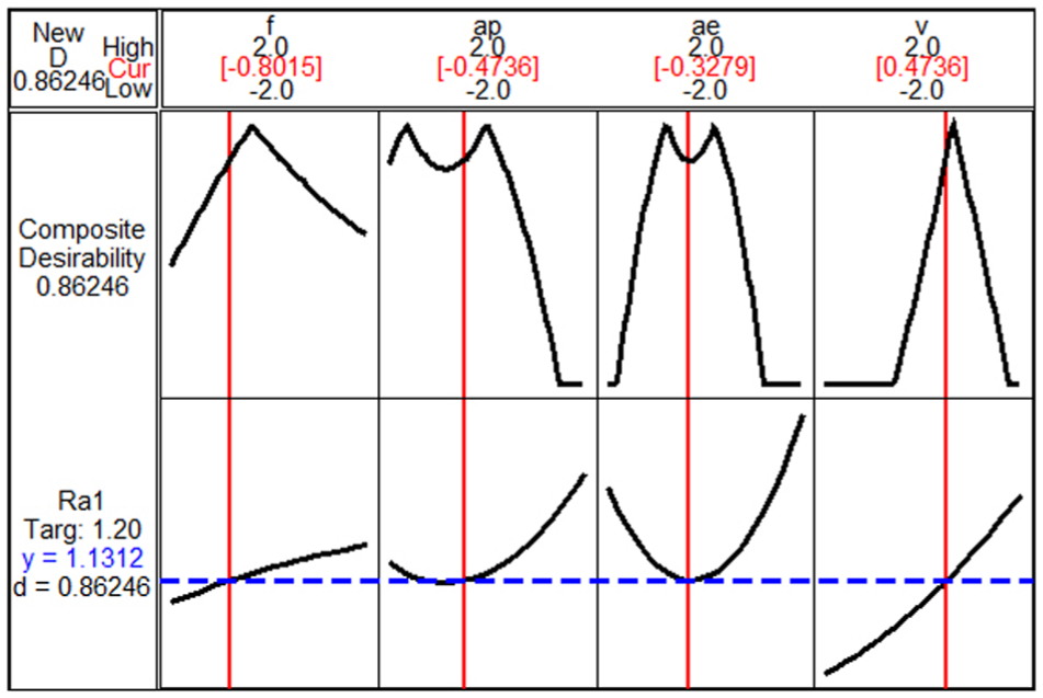
Optimization results for surface roughness using composite desirability function.

Table 7.

Optimal solution of process parameters and surface roughness through RSM and TLBO.

Approaches	Goal	Optimum combinations				Target	Upper limit	Predicted response	Desirability
Approaches	Goal	f_z (mm/tooth)	A_p (mm)	A_e (mm)	V_c (m/min)	Target	Upper limit	Predicted response	Desirability
Composite desirability	Minimum	0.08	0.81	0.32	136.75	0.9	1.8	1.13	0.86
TLBO	Minimum	0.06	0.74	0.38	145.8		1.8	1.11	–

TLBO: teaching-learning-based optimization.

Optimization using TLBO

The detailed procedures for implementation of TLBO are stated as follows:

1. Define the optimization problem

$Minimize : R_{a} (f_{z}, A_{p}, A_{e}, V_{c})$

Subjected to: $\begin{matrix} 0.02 mm / tooth \leq f_{z} \leq 0.22 mm / tooth, \\ 0.2 mm \leq A_{p} \leq 1.8 mm \\ 0.1 mm \leq A_{e} \leq 0.9 mm, \\ 75 m / \min \leq V_{c} \leq 175 m / \min \end{matrix}$

The developed mathematical model for surface roughness shown in equation (11) has been used as fitness function of TLBO for minimization. The constraints are feed per tooth (f_z), cutting speed (V_c), and axial and radial depth of cut (A_p and A_e, respectively).

2. Initialize the population

In the second step, a random population is generated according to population size and number of cutting parameters. Learners represent population size and subjects represent the cutting process parameters in TLBO. The cutting process parameters are used to generate a random initial population.

3. Teacher phase solution

4. Learner phase solution

5. Termination criterion.

The program will be terminated when the maximum generation number is achieved; otherwise, it will again start from step 3 and will continue till the maximum generation number is achieved. In this article, Deb’s heuristic constraint handling method has been adopted to handle the constraints in the problem. Initially, various trails have been carried out by running TLBO algorithm for different population sizes, numbers of generations, and teaching factor to get the consistent results. The optimum result has been obtained at 20 population size, 100 number of generations, and in 10 iterations. Teaching factor has been selected 2 after numerous trails. The obtained result is shown in Table 7.

The obtained optimum result for surface roughness is 1.11 µm. The global optimum value for the surface roughness is obtained at run no. 67. The corresponding optimum actual values of the cutting parameters are shown in Table. 8.

Table 8.

Confirmation tests in actual values and its results.

Exp. trial	f_z (mm/tooth)	A_p (mm)	A_e (mm)	V_c (m/min)	Predicted R_a (µm)	Experimental R_a (µm)
CD	0.08	0.81	0.32	136.75	1.13	1.21
TLBO	0.06	0.74	0.38	145.8	1.11	1.16
16	0.17	1.4	0.7	150	2.44	2.38
25	0.12	1	0.5	125	1.10	1.18

CD: composite desirability function; TLBO: teaching-learning-based optimization.

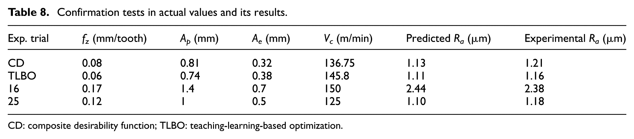
Four confirmation experiments have been carried out to verify the adequacy of the developed model. The predicted and experimental values of the confirmation tests are shown in Table 8. First two tests are performed with the optimal cutting parameters obtained by composite desirability function (CD) and TLBO. Other two test conditions have been selected from the previous experimental plan (from Table 4). It can be seen that predicted results and experimental results are very close to each other. It may also be observed that the TLBO method yields better optimization compared to composite desirability approach.

Conclusion

In this article, mathematical modelling of surface roughness for HSM milling has been carried out in terms of feed per tooth, cutting speed, axial depth of cut, and radial depth of cut. A second-order full quadratic model developed is reasonably adequate and may be used for prediction of surface roughness within the ranges of the cutting parameters using RSM. However, the following conclusions have been drawn from the present work:

ANOVA of individual parameters revealed that cutting speed is the most significant parameter influencing the surface roughness accounting 47.18% contribution. Surface roughness increases with the increase in cutting speed.

Feed per tooth, axial depth of cut, and radial depth of cut have also significant effect on surface roughness accounting 4.11%, 10. 83%, and 4.92% contributions, respectively. The interaction terms are found to be insignificant.

Surface roughness continuously increases with the increase in feed per tooth keeping other parameters unchanged. From the three-dimensional (3D) surface plot, it is found that the surface roughness decreases when radial depth of cut increases from 0.1 to 0.5 mm, and increases when radial depth of cut increases from 0.5 to 0.9 mm.

The optimization using TLBO methodology took minimum effort and provided better results. The optimal parametric setting obtained by TLBO has been verified through experiments. Thus, the method is an efficient method and may further be employed for optimization of cutting forces and material removal rate in HSM process.

Footnotes

Appendix 1 Acknowledgements

The experimental work was carried out using Vertical Milling Centre in Manufacturing Technology Laboratory, CSIR-CMERI Durgapur, India. The authors acknowledge the support extended by Mr S.Y. Pujar for his assistance in conducting experiments.

Declaration of conflicting interests

The author(s) declared no potential conflicts of interest with respect to the research, authorship, and/or publication of this article.

Funding

The author(s) received no financial support for the research, authorship, and/or publication of this article.

References

Sonawane

Joshi

SS.

Analytical modelling of chip geometry and cutting forces in helical ball end milling of super alloy Inconel 718. CIRP J Manuf Sci Technol 2010; 3: 204–217.

Benardos

Vosniakos

GC.

Predicting surface roughness in machining: a review. Int J Mach Tool Manu 2003; 43: 833–844.

Sriyotha

Sahasrabudhe

Yamazaki

et al . Geometrical modelling of ball end finish milling process for a surface finish. Proc IMechE, Part B: J Engineering Manufacture 2006; 220: 467–477.

Liu

Loftus

Prediction of surface quality from ball-nose milling in high speed machining applications. Proc IMechE, Part B: J Engineering Manufacture 2006; 220: 571–578.

Fuh

CF.

A proposed statistical model for surface quality prediction in end-milling of Al alloy. Int J Mach Tool Manu 1995; 35(8): 1187–1200.

Alauddin

El Baradie

Hashmi

MSJ

. Computer-aided analysis of a surface-roughness model for end milling. J Mater Process Tech 1995; 55: 123–127.

Alauddin

El Baradie

Hashmi

MSJ

. Optimization of surface finish in end milling Inconel 718. J Mater Process Tech 1996; 56: 54–65.

Monsour

Abdalla

CEnf

Surface roughness model for end milling: a semi-free cutting carbon casehardening steel (EN32) in dry condition. J Mater Process Tech 2002; 124: 183–191.

Lin

TR.

Experimental design and performance analysis of TiN-coated carbide tool in face milling stainless steel. J Mater Process Tech 2002; 127: 1–7.

10.

Vivancos

Luis

Costa

et al . Optimal machining parameters selection in high speed milling of hardened steels for injection moulds. J Mater Process Tech 2004; 155–156: 1505–1512.

11.

Batista

Rodrigues

Coelho

RT.

Modelling and characterisation of roughness of moulds produced by high- speed machining with ball nose end mill. Proc IMechE, Part B: J Engineering Manufacture. Epub ahead of print 5 May 2015. DOI: 10.1177/0954405415584898.

12.

Wang

Chang

HY.

Experimental study of surface roughness in slot end milling AL2014-T6. Int J Mach Tool Manu 2004; 44: 51–57.

13.

Ginta

Amin

AKN

Mohd Radazi

HCD

et al . Development of surface roughness model in end milling Titanium alloy Ti-6Al-4V using uncoated carbide inserts. Eur J Sci Res 2009; 28(4): 542–551.

14.

Ding

Zhang

Wang

et al . Empirical model and optimal cutting parameters for cutting forces and surface roughness in hard milling of AISI H13 steel. Int J Adv Manuf Tech 2010; 51: 45–55.

15.

Bhardwaj

Kumar

Singh

PK.

Effect of machining parameters on surface roughness in end milling of AISI 1019 steel. Proc IMechE, Part B: J Engineering Manufacture 2014; 228(5): 704–714.

16.

Montgomery

DC.

Design and analysis of experiments. 4th ed. New York: Wiley, 1997.

17.

Rao

Savsani

Vakharia

DP.

Teaching–learning-based optimization: a novel method for constrained mechanical design optimization problems. Comput Aided Design 2011; 43: 303–315.

18.

Rao

Savsani

Vakharia

DP.

Teaching–learning-based optimization: an optimization method for continuous non-linear large scale problem. Inform Sciences 2012; 183: 1–15.

19.

Rao

Kalyankar

VD.

Parameter optimization of modern machining processes using teaching–learning- based optimization algorithm. Eng Appl Artif Intel 2013; 26: 524–531.

20.

Rao

Patel

An elitist teaching–learning-based optimization algorithm for solving complex constrained optimization problems. Int J Ind Eng Comput 2012; 3(4): 535–560.

21.

Baghlani

Makiabadi

MH.

Teaching-learning-based optimization algorithm for shape and size optimization of truss structures with dynamic frequency constraints. IJST Trans Civ Eng 2013; 37: 409–421.

22.

Puri

Banerjee

Multiple-response optimisation of electrochemical grinding characteristics through response surface methodology. Int J Adv Manuf Tech 2013; 64: 715–725.

23.

Derringer

Suich

Simultaneous optimization of several response variables. J Qual Technol 1989; 12: 214–219.

24.

Sreejith

Ngoi

BK.

Dry machining: machining of the future. J Mater Process Tech 2000; 101: 287–291.