
Abstract
Contrary to the conventional serial kinematics machine tools, the parallel kinematics machine tools exhibit nonlinear behavior which is a major source of the machining error. This causes even a linearly programmed path to be traversed along a nonlinear path. The resulting error, known here as the kinematic error, should be critically considered during the toolpath planning. The estimation of the maximum kinematic error using the concept of median osculating circle is introduced in this article. The proposed formulation demonstrates that the maximum kinematic error depends on the curvature of the actual trajectory. In order to estimate the curvature, constant curvature contour maps are introduced. These maps depend on the structural parameters of the machine and are recommended to be provided by the machine’s manufacturer. The constant curvature contour maps are illustrated to be an effective graphical tool for kinematic error estimation and thus successfully conducting the optimal planning of the toolpath and the workpiece setup. Consequently, it is recommended in this article that the constant curvature contour maps be employed in the format of a database by computer-aided manufacturing systems during toolpath planning and by interpolators during command generation or by a part programmer to optimally setup the workpiece or conduct the toolpath planning such that the least kinematic error occurs during the machining.
Keywords
Introduction
Parallel kinematics (PK) mechanisms have found extensive applications in various industries 1 such as machine tools. 2 A major drawback of parallel kinematics machine (PKM) tools is their nonlinear behavior. It has been established in the literature that the kinematics of parallel mechanisms map linear relations inside the actuators’ space into nonlinear relations inside the end effector’s space.3–6 In other words, the upper platform in a hexapod machine tool moves along a nonlinear path although the pods are linearly actuated by servo drives. The nonlinear behavior of the PK mechanisms significantly affects the accuracy of the interpolated toolpaths. Contrary to PKMs, the straightness in serial kinematics (SK) machine tools can be obtained along Cartesian axes, and out of straightness is mainly attributed to the malfunction of mechanical elements. This has been verified by Altintas et al. 7 who illustrated that the SK machine tools exhibit linear behavior and a linear toolpath is provided by simply generating linear commands to axes’ drives. It is noteworthy that the guide-ways in SK machine tools represent the Cartesian axes and act as prismatic joints. The nonlinearity of parallel mechanisms has been investigated by some researchers. Jinsong et al. 3 employed Bates and Watts measures of nonlinearity for analysis of the accuracy of interpolated toolpaths. Karimi and Nategh 4 employed the same measures to conduct statistical investigation into the effect of toolpath parameters. Wang et al. 5 employed singular values of the Jacobian matrix to predict the interpolation error resulting from the kinematic nonlinearity of a 3-degree-of-freedom (DOF) PKM tool. Zheng et al. 6 introduced the middle sampling interpolation algorithm to limit the interpolation error for a 5-DOF PKM tool. They also showed that when the cutting tool is commanded to move linearly, it moves along a circle-like trajectory. Jinsong et al. 3 also achieved the same result.
The planning of optimal toolpath and workpiece setup inside the workspace of PKM tools has been widely investigated by researchers from the viewpoints of singularity avoidance, and optimization of the force, energy, time, and stiffness. Khoukhi et al. 8 presented an approach for the multi-objective dynamic trajectory planning of PKMs under task, workspace, and manipulator constraints. In the proposed trajectory planning method, the electrical energy, the kinetic energy, and robot traveling time separating two sampling periods were minimized, and a measure of manipulability allowing singularity avoidance was maximized. Dasgupta and Mruthyunjaya 9 addressed the problem of singularity-free path planning. An algorithm has been developed to construct continuous paths within the workspace of the manipulator by avoiding singularities and ill-conditioning. Given two end-poses of the manipulator, the algorithm finds out safe (well-conditioned) points and plans a continuous path from the initial pose to the final one. Dash et al. 10 determined the singularity points within the reachable workspace of the parallel manipulators, grouped them into several clusters, and modeled them as obstacles. A path planning algorithm was employed to find an optimal path avoiding these obstacles. Lin et al. 11 proposed a singularity avoidance approach of the path planning scheme based on a DNA evolutionary computing algorithm whose coding technique successfully speeded up the execution of search for fast path generation within the feasible workspace. Oen et al. 12 presented the synthesis of the point-to-point trajectory of the moving platform such that the distribution of the cutting force of the tool bit along a specified machining contour is optimized. Shaw and Chen 13 employed the genetic algorithm to minimize the six axial forces of the Stewart-platform-based milling machine at every contact point, while using the iso-scallop method in the process of generating the cutting path. Plessis and Snyman 14 conducted the optimal trajectory planning by minimizing the dynamic actuator forces required for executing the prescribed path, subject to constraints on the geometry and the ranges of actuator lengths. Kumar et al. 15 developed a stiffness model for contour generation application to identify the trajectory with maximum stiffness for complex contours in a reconfigurable Stewart platform. Harib et al., 16 employed a knowledge-based approach, which used a set of qualitative rules among the input and output parameters, to conduct the optimal trajectory planning. In their work, the condition number of the Jacobian was adopted as the objective function. The minimization of the objective function provided six coordinates of the end effector of their manipulator. Zhang et al. 17 introduced the mean value and the standard deviation of the trace of the generalized compliance matrix as two global compliance indices. They illustrated that the mean value represented the average compliance of the PKM over the workspace, while the standard deviation indicated the compliance fluctuation relative to the mean value. They presented several compliance mappings, which can be employed during toolpath planning of the developed PKM. Afroun et al. 18 first approximated the time evolution of the mobile platform, Cartesiancoordinates, and the orientation by cubic spline functions with free control points and then employed the sequential quadratic programming to optimally determine the position of the control points as well as the transfer time. Pateloup et al. 19 discussed the optimal location of a trajectory inside the workspace of PKM tool to minimize the machining time. However, they neglected the kinematic nonlinearity and the consequent machining error. Smirnov et al. 20 investigated the optimal trajectories for PKM tools considering the energy optimization. Chen and Pham 21 proposed a planning process which minimized the traverse time and expended energy subject to various constraints imposed by the associated kinematics and dynamics of the manipulator. Pugazhenthi et al. 22 proposed an optimal trajectory planning scheme for Stewart-platform-based machine tools in which the stiffness of the structure was maximized and simultaneously the force requirement of the actuators was minimized, while satisfying the constraints of workspace and singularity. Muruganandam and Pugazhenthi 23 presented a methodology to plot the workspace atlas based on stiffness for hexapod machine tools. They also demonstrated how such stiffness-based workspace atlas could help in selecting optimal workpiece location. Kim and Sarma 24 showed that the performance envelope of a machine at a point on the surface is very anisotropic. They introduced the greedy approach, for obtaining the directions of the best performance. Wang et al. 25 studied the effects of geometric and non-geometric constraints on the Stewart platform workspace based on which they reported how to determine the pose of a workpiece in a parallel machine tool. Song and Mou 26 proposed a method to find the near-optimal part setup position and orientation based on the workspace, stiffness, and accuracy capability of a PKM that could be used for 5-axis machining.
The nonlinear behavior of PKM tools requires special attention during part programming. The intensity of nonlinearity varies within the machine’s workspace. The optimal placement of the workpiece inside the workspace of PKM tool is, therefore, of special importance for avoiding intense nonlinearities which can lead to unacceptable machining tolerances and increase in scraps. The optimal setup of workpiece alleviates the need to decrease the interpolation step. The decrease in interpolation step can encounter technical limitation of the controller and require the feed-rate to decrease. The decrease in feed-rate results in its distancing from the optimal value and leads to decrease in productivity.
The PKM tool’s part programmer should have a clear idea about the optimal setup of the workpiece within the machine’s workspace before he can decide the machining strategy and the desired toolpath. This requires that the part programmer has a proper understanding of the way the nonlinearity of the PKM changes over the workspace. The change of nonlinearity within the workspace of a PKM tool is, however, much complicated and far beyond the part programmer’s grasp. Actually, he is not required to think about the kinematics of the machine when programming a toolpath for a SK machine tool. He should equally be excused from dealing with the kinematics of the PKM when programming the toolpath. Therefore, he needs a handy little tool to aid him with quickly grasping the change pattern of the nonlinearity. Although both optimal toolpath/workpiece setup and the nonlinearity of PKMs have been discussed in the literature, no significant work has been presented considering the optimal workpiece location regarding the kinematic nonlinearity of PKMs. A map demonstrating the change pattern of nonlinearity can perform the role of this tool. It can make it as a visual aid. The constant curvature contour (CCC) maps proposed in this study are quite appropriate for this purpose, which can graphically present an estimate of the maximum kinematic error occurring along a given toolpath. It is envisaged that the CCC maps would be eligible to be embodied in a database inside computer-aided manufacturing (CAM) software for use in toolpath planning in hexapod machine tools. The introduction of CCC maps is the main novelty of this article. The CCC maps depend on the structural parameters of the machine such as the location of the spherical and universal joints, as well as the height of the UP at the home position. Therefore, CCC maps are recommended to be provided by the hexapod machine tool manufacturers.
Kinematic nonlinearity and maximum kinematic error estimation
The kinematics of the PKMs have been illustrated to be nonlinear. 27 During the trajectory generation, such a nonlinear behavior brings about kinematic error. 28 The kinematic error is defined as the distance between the actual position of the UP and its position where it is commanded to be at a specified position. The workspace of the PKMs is known to be inhomogeneous in terms of stiffness, dexterity, and kinematic nonlinearity, which makes the optimal workpiece setup a nontrivial problem. The heavy computational burden makes it technologically almost impossible to incorporate the analytical calculations into the real-time interpolation algorithms. Some attempts by Muruganandam and Pugazhenthi 23 have been made to introduce a graphical means to conduct the optimal workpiece setup.
Although the kinematic error concept is developed for the platform at a specific position, it can be readily applied to the UP trajectories as the trajectory is discretized into a finite sequential number of points. Karimi and Nategh 28 presented the hexapod kinematic error model and mathematically demonstrated that the kinematic error depends not only on the UP position but also on the trajectory parameter (the distance between the start and end points of the trajectory). The same phenomenon has also been illustrated in Jinsong et al. 3 and Karimi and Nategh 4 separately. The constant curvature curves are introduced in this section to provide a graphical tool for planning the toolpath and workpiece setup. The constant curvature curves take the advantage of estimating the maximum kinematic error for a toolpath using the concept of the median osculating circle (MOC) as follows.
When the UP moves between two points, it is observed from the derivative plot of the kinematic error along the trajectory for numerous examples that the derivative decreases almost linearly and crosses the abscissa only once and at the middle of the trajectory’s length. Based on this observation, a hypothesis is proposed that when actuators elongate with constant speed, the actual trajectory of the UP can be approximated by a circular path as shown in Figure 1. Such an observation has already been published by Jinsong et al. 3 and Zheng et al. 6 The geometrical difference between the desired and actual trajectories is the kinematic error whose maximum value is denoted by e*. It is known that e* happens almost at the middle of the trajectory. The osculating circle at the midpoint of the actual trajectory, named as MOC, is shown in Figure 1(a). The radius of MOC is the reciprocal of the curvature of the actual trajectory at its midpoint. Although no analytical information for the actual trajectory is available, the curvature at the midpoint can be readily calculated from the forward kinematics formulation of velocity and acceleration.
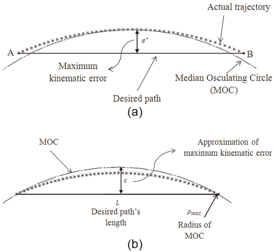
Estimation of maximum kinematic error using MOC: (a) desired path, actual trajectory, and the MOC and (b) shift of MOC.
Figure 1(a) shows that MOC osculates the actual trajectory at the midpoint and might not pass through the beginning and end points of the trajectory (points A and B, respectively). It should be noted that the actual and the desired trajectories meet each other at these two points. Provided that the desired path’s length is smaller than the diameter of osculating circle, which is the case for trajectories with common speeds in machining, MOC can be moved such that it intersects with the desired path at both A and B points as shown in Figure 1(b).
Based on the concept introduced in Figure 1(b), the maximum kinematic error can be calculated as follows
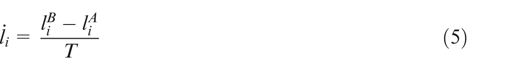
where ε is an approximate of the maximum kinematic error for the desired path, ρMOC is the radius of MOC, L is the path length, and κ* is the curvature of the path at the midpoint. The curvature κ* can be obtained as follows
where

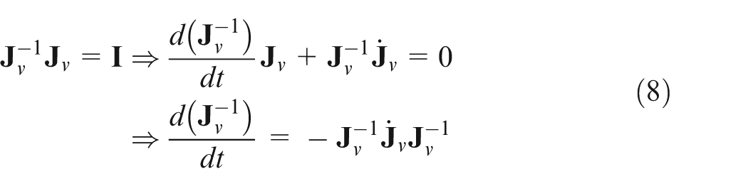
where
where
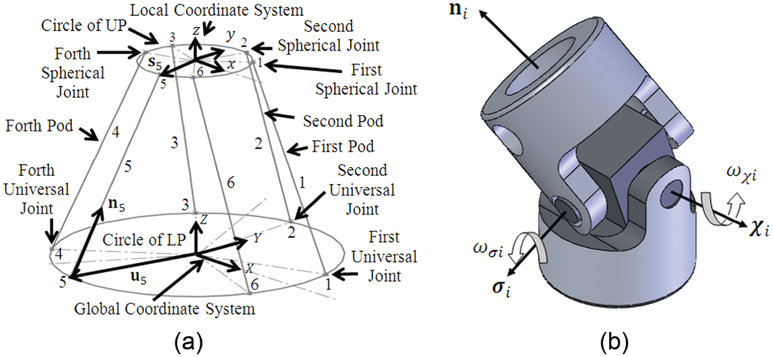
Hexapod mechanism: (a) the kinematic chains and (b) the rotation axes of universal joints.
where
where v is the velocity of UP during its travel from points A to B.
The derivative of equation (3) yields the acceleration as follows
where
Substituting equation (8) into equation (7) yields

where
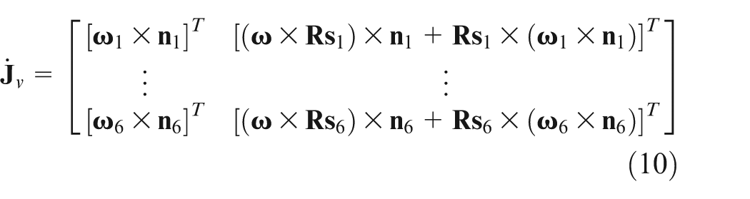
where

where
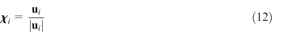
where
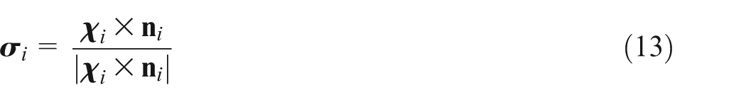
where ωχi and ωσi are obtained as follows (these terms are first presented by Harib and Srinivasan 27 )
where
CCC maps
Equation (1) illustrates that the length of the desired toolpath and the curvature of the actual trajectory at its midpoint directly govern the kinematic error. The length of the desired toolpath is an independent parameter, while the curvature of the actual trajectory at its midpoint depends on parameters of the desired toolpath such as the location of its midpoint, as well as its orientation and length. It is shown in the Appendix 2 that the UP travel speed also referred to as feed-rate has no effect on the curvature.
The CCC maps (Figures 3 and 4) illustrate the variation of κ* inside the workspace. To obtain plots of this figure, all types of toolpaths (horizontal, vertical, and inclined toolpaths) are examined. The curvature κ* is calculated by determining pods’ elongation rate from equation (5); the UP velocity and acceleration vectors from equations (3) and (9), respectively; and assuming


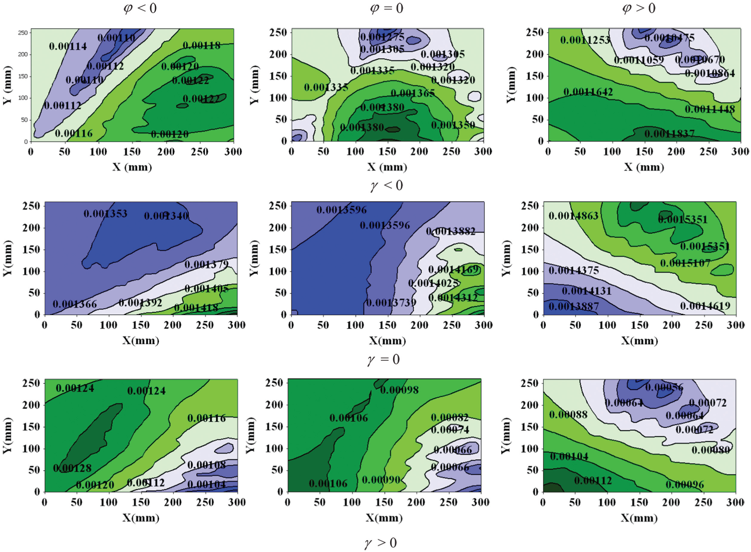
CCC maps for z = 700 mm and L = 150 mm.
CCC for a vertical toolpath (γ = 90°) for z = 700 mm.
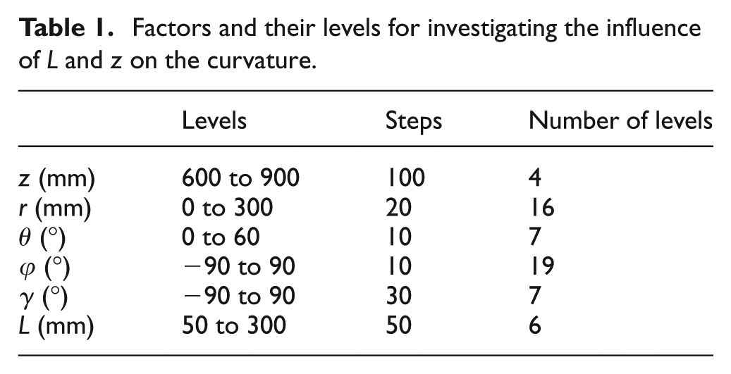
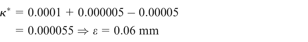
Figures 3 and 4 have been plotted for z = 700 mm and L = 150 mm. To consider the effect of z and L on the curvature, a comprehensive investigation has been conducted. In this investigation, the relevant parameters with the levels presented in Table 1 and their permutations were taken into account. The corresponding curvature was calculated for each toolpath. It was evidenced that L and z had no interaction with the rest of the factors. The results are depicted in Figure 5. It is clear from this figure that an increase in L leads to the decrease in the curvature. A similar trend is also observed for the influence of z on the curvature. In Figure 5, κ* is the mean value of the curvature obtained by considering different levels of the rest of the factors.
Factors and their levels for investigating the influence of L and z on the curvature.
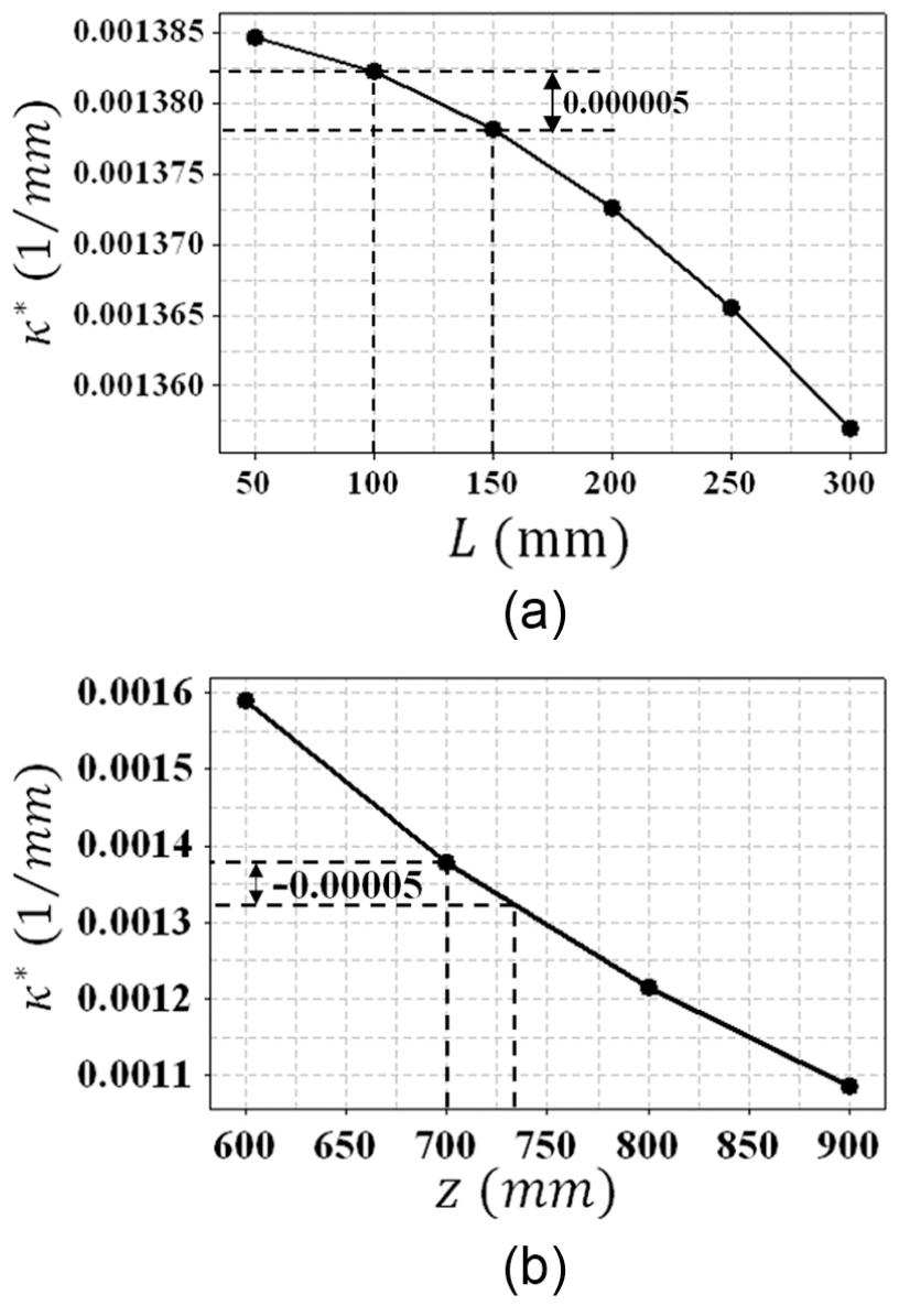
Plot of curvature versus (a) length and (b) height of the actual trajectory.
Illustrative example
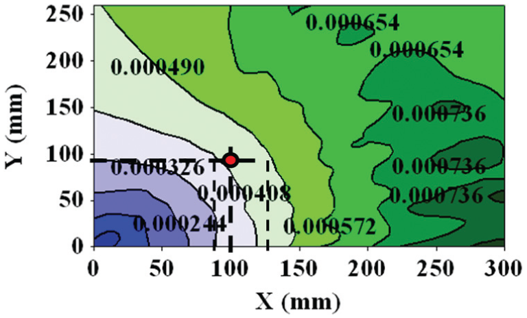
Figures 3–5 provide a tool to estimate the maximum kinematic error and choose the region with less kinematic error. This way the planning of the optimal toolpath planning or workpiece setup can be performed by a part programmer. A database can also be developed based on the information provided by Figures 3–5, to be employed by CAM software. The remainder of this section provides an illustrative example which demonstrates how CCC maps can be employed to optimally locate a toolpath.
A vertical toolpath (corresponding to machining operations such as drilling, reaming, and vertical boring) is considered with its midpoint at

Replacing κ* = 0.000383 (mm−1) and L = 100 mm into equation (1) yields ε = 0.48 mm.
Figure 4 suggests that placing the toolpath closer to the origin decreases the kinematic error. If the toolpath is moved to the location
Figures 3 and 4 present the curvature of the toolpaths whose midpoints are situated in the first region of symmetry. The hexapod consists of six areas of symmetry
28
as depicted in Figure 6. For the toolpaths whose midpoints are not located in the first region of symmetry, the equivalent of these midpoints in the first area should be found prior to using the CCC maps. This is done with the aid of the principle axes of symmetry. For example, for the point
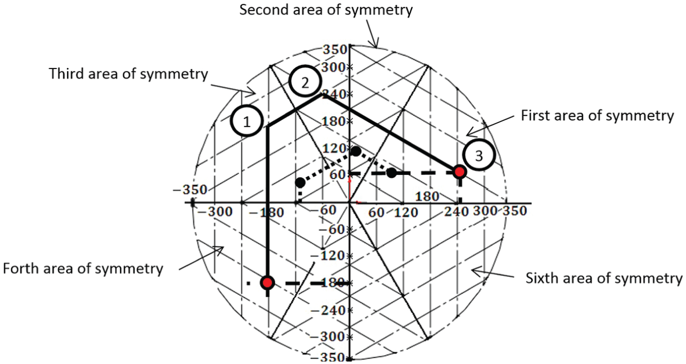
Guidelines to find symmetrical equivalents.
Experimental setup and verification
The hexapod machine manufactured in this research as shown in Figure 7 consists of a Stewart platform mechanism, a PC on which an interface (human–machine interface (HMI)) is installed, a motion controller, and six servo systems including servo drives and servo motors. The interface developed by the authors is programmed in Visual C# and is capable of interpreting the G-code commands based on ISO 6983. Motion controller is a real-time module and is capable of controlling six servo systems simultaneously. Commands are input using G-code standard. The HMI interprets the command, solves the inverse kinematics, and sends the data corresponding to the six pod lengths to the motion controller. The motion controller provides the six servo drives with the appropriate voltage as the servo input command and receives the feedback from the servo encoders to close the position control loop. The velocity control loop is closed in the servo drive. A proportional–proportional–integral (P-PI) controller has been developed for the machine. The P-controller is applied to the position control loop and the PI-controller is applied to the velocity control loop. The system dynamic characteristics are identified experimentally in this research and the controller gains are tuned correspondingly. The Stewart mechanism as described earlier has six universal and six spherical joints. The six universal joints are arranged on a circle with the radius of 634.24 mm on lower platform, identified after calibration. 29 Each pair of universal joints has an angular distance of 40° from each other and each pair is 120° away from the adjacent one. The six spherical joints are also arranged around a circle on the UP with the radius of 250.93 mm, after calibration. They are also arranged in pairs. Each pair of spherical joints has an angular distance of 85° from each other and pairs are 120° away. To measure the position of UP during its motion, an optical pair of digital cameras is used. The cameras take a picture from two perpendicular directions from a target installed on UP every 1/30 of a second. The side camera is carefully aligned normal to yz-plane of the machine and the front camera is also aligned normal to xz-planes of the machine. The films recorded by the cameras are processed using image correlation function embedded in MATLAB to obtain the location of the target every 1/30 of a second.
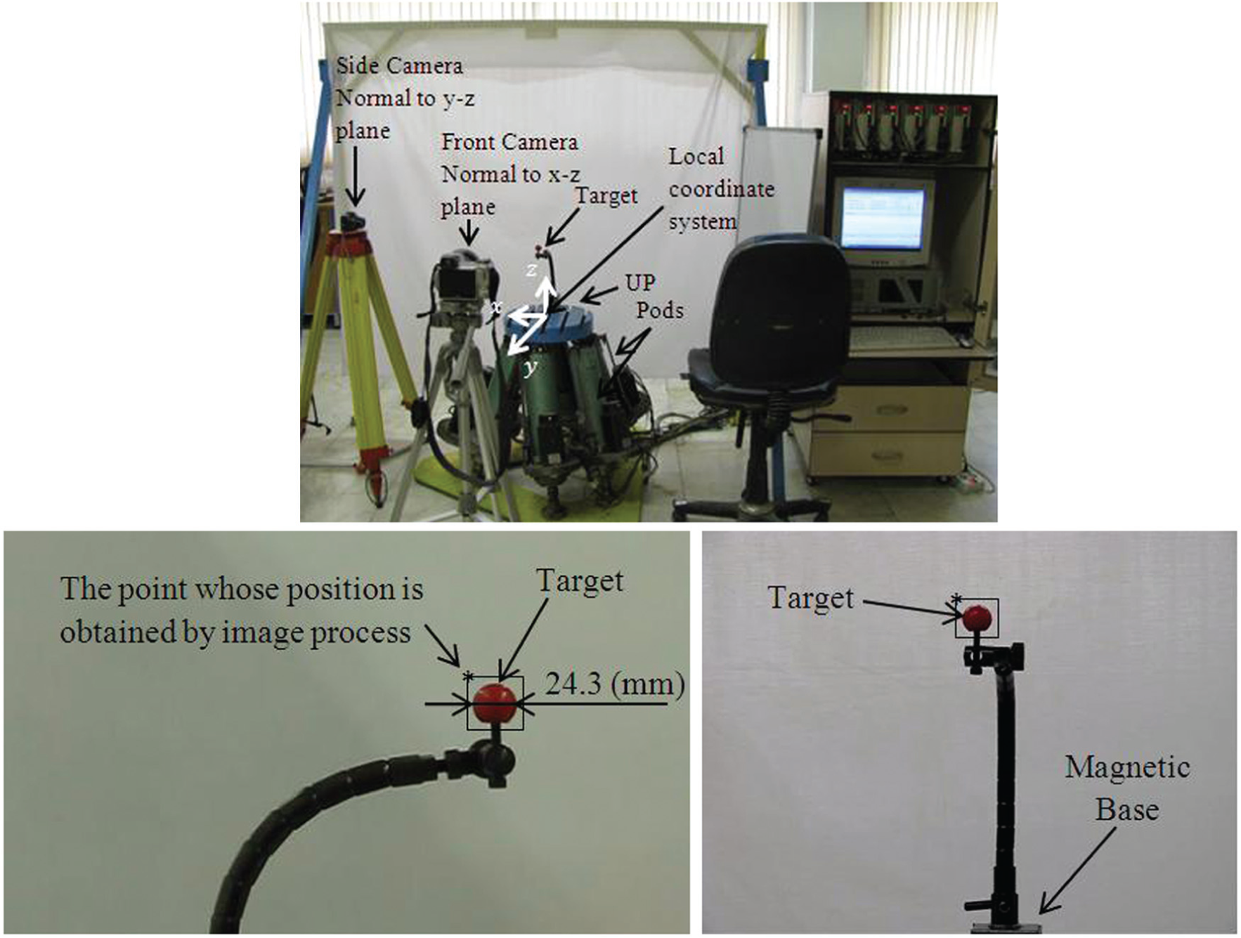
Experimental setup.
The image correlation output is obtained in terms of pixels, which is calibrated using the target whose diameter is 24.3 mm. Measuring the number of pixels occupied by the target in the images recorded by side and front cameras revealed that the resolution of displacement measurement during the experiments varied from 0.4 to 0.7 mm for front camera depending on the zoom of the camera and 0.3 to 0.5 mm for the side camera.
The Taguchi L18 standard array has been employed for the design of experiments. The length and the location of the midpoint together with the orientation of the toolpath are the relevant factors in the design of experiments. The values of factors, and the experimental and theoretical results are presented in Table 2. Each run of the experiment indicates a toolpath with unique parameters. The maximum kinematic error is measured for each toolpath. The experimental measurements are compared with the maximum kinematic error obtained from equation (1) based on the concept of MOC. The curvature is obtained from the CCC maps presented in Figures 3 and 4. For the toolpath with the length and height of midpoint other than L = 150 mm and z = 700 mm, Figure 5 is used to adjust the values of the curvature obtained from CCC maps.
Maximum kinematic error for different toolpaths.
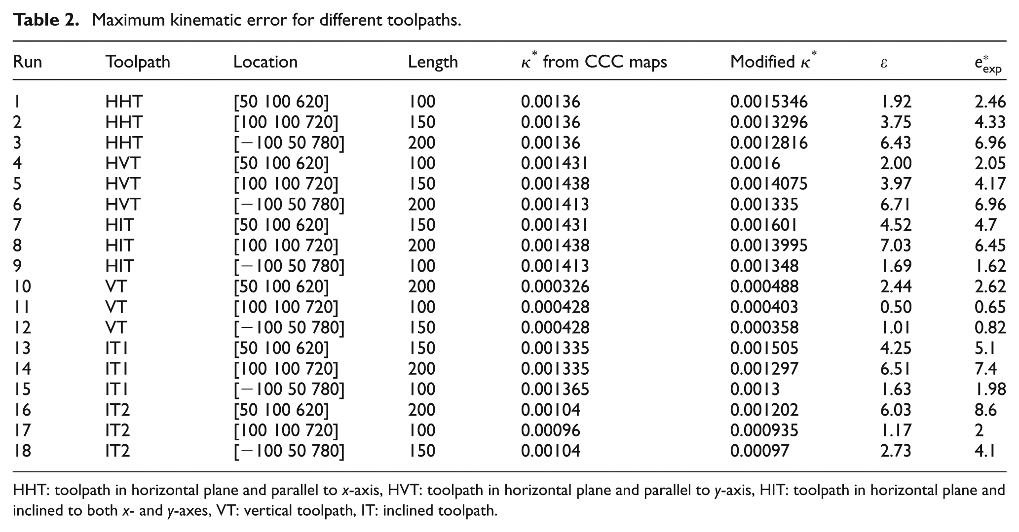
HHT: toolpath in horizontal plane and parallel to x-axis, HVT: toolpath in horizontal plane and parallel to y-axis, HIT: toolpath in horizontal plane and inclined to both x- and y-axes, VT: vertical toolpath, IT: inclined toolpath.
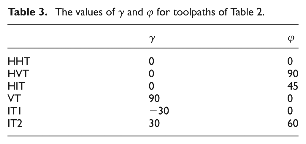
The angles γ and ϕ which describe the toolpath’s orientation are presented in Table 3 for the toolpaths of Table 2.
The values of γ and φ for toolpaths of Table 2.
The experimental results and the theoretical approximate results for the maximum kinematic errors are illustrated in Figure 8. The difference between the results has also been indicated on this figure in percentage. From this figure, it can be seen that the maximum discrepancy between the results is 27.3%. The average estimation error for the 18 toolpaths is 11.3%.
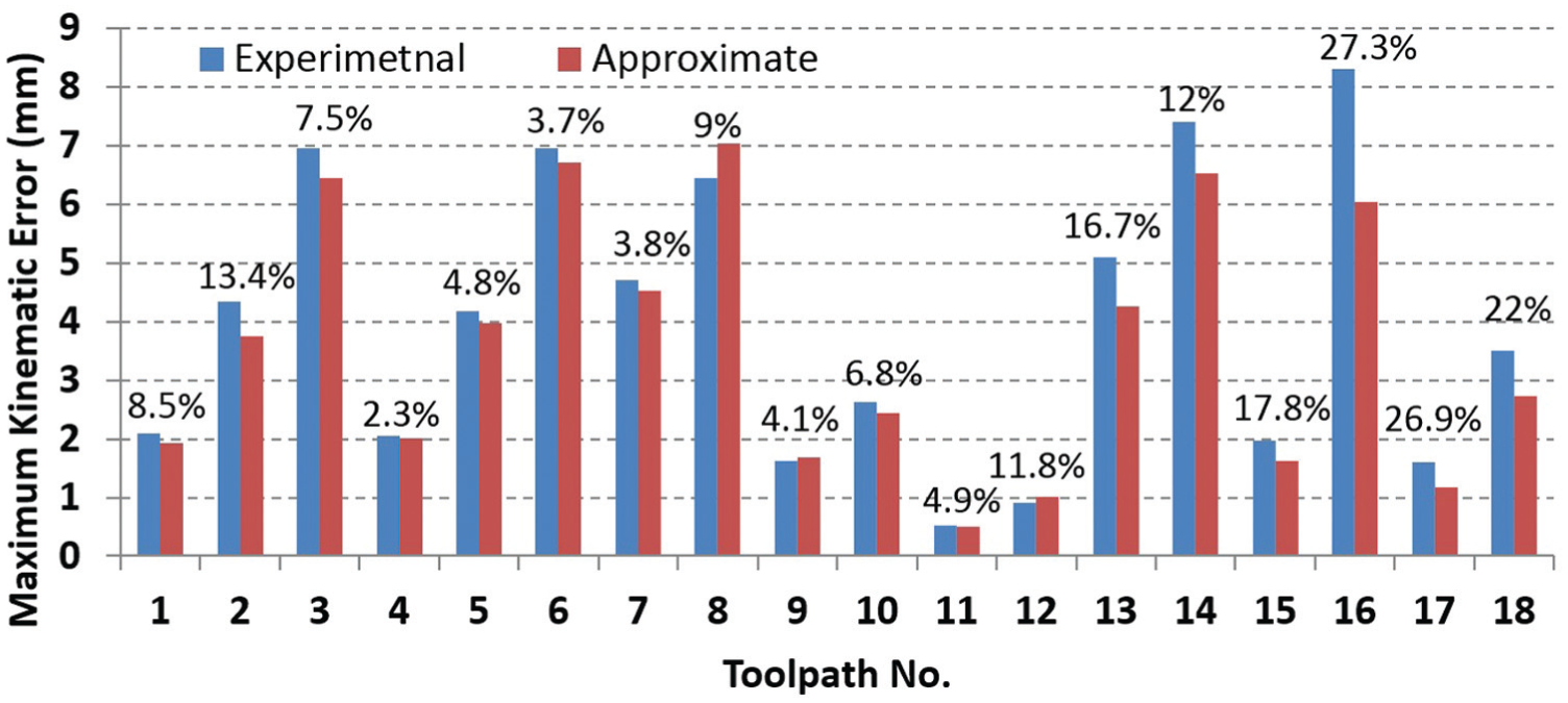
The experimental and theoretical values of the maximum kinematic error.
The sources of inaccuracies are mainly the errors of the measurement procedure, as well as the inaccuracies inherent in the manufacture of the machine structure. Although the calibration has been performed on this structure in a previous work 29 and applied to the interpolation procedure of the machine, some errors still exist due to the manufacturing and calibration inaccuracies as reported in Nategh and Agheli. 29 Details of the error sources are elaborated in Nategh and Agheli 29 for this structure.
Conclusion
An analytical tool has been developed for approximating the maximum kinematic error of hexapod machine tools on the basis of MOC.
CCC maps were introduced in this article to quickly and graphically find the curvature of the actual trajectory. The CCC maps provide a means to estimate the kinematic error inside the workspace and thus enable a part programmer to optimally setup the workpiece. The manufacturers of the hexapod machine tools can provide the users with CCC maps as an aid to the part programmer.
It was also analytically shown that the upper platform’s travel speed has no effect on the curvature of the actual trajectory and thus has little effect on the maximum kinematic error.
It was shown that generally as the toolpath inclines more toward a horizontal plane, a poorer estimation tends toward the border of the workspace. A better estimation is obtained near the horizontal x-axis of the machine for the toolpaths whose projections on the horizontal xy-plane make small angle with this axis. The poorer estimation moves away from the x-axis as this angle increases.
The presented formulation and method were experimentally verified. The average discrepancy between the experimental and theoretical results was about 11%, while its maximum was about 27%.
Footnotes
Appendix 1
Appendix 2
Declaration of conflicting interests
The authors declare that there is no conflict of interest.
Funding
This research received no specific grant from any funding agency in the public, commercial, or not-for-profit sectors.