Topology face–based change propagation analysis in aircraft-assembly tooling design

Abstract

Assembly tooling design is implemented according to the constraints of geometric information and technical requirements of aircraft. Changes in aircraft parts will cause changes in assembly tooling parts. Using topology faces as basic processing units and focusing on the constraint relationships between topology faces, this article presents a method for change propagation analysis from aircraft to assembly tooling, which assists designers to detect changes efficiently and assess the change influence qualitatively in a uniform way. First, change vector representing the change state of the original parts’ topology faces and relation matrix recording the relationships between the topology faces are introduced. Then, based on the change vectors and relation matrices, an algorithm is developed to obtain the overall geometrical change propagations from aircraft parts to assembly tooling parts. Meanwhile, a concept of change influence index is presented to evaluate the change qualitatively. Finally, a computer-aided system is developed and the proposed change propagation analysis method is demonstrated by applying it to an aircraft-assembly tooling.

Introduction

Aircraft-assembly tooling plays an important role in guaranteeing the required location and orientation of aircraft subassemblies and parts according to the design specifications. Assembly tooling parts are large in amount and complex in structure. Instead of the traditional process of product development, which is highly procedural, a high-performance design method is defined by the following key terms, “dynamic,”“concurrent,”“distributed” and “collaborative.” ¹ Accordingly, aircraft design and assembly tooling design are also carried out concurrently. Due to the customer requirements, technology innovation, mistakes and so on, design change in aircraft occurs frequently. Thus, the frequency of design change in the assembly tooling caused by design change in aircraft may increase significantly. Besides, the numerous parts of assembly tooling and complex relationships between aircraft parts and assembly tooling parts make the change management a time-consuming and effort-consuming task. Traditionally, an assembly tooling designer is informed about aircraft design changes, and then makes a decision on the assembly tooling parts which need to be changed by his or her own experiences. Due to the complex geometrical constraints between aircraft parts and assembly tooling parts as well as the possibility of change propagation, such manual change management way may cause the assembly tooling designers to omit some changes in parts and delay the development cycle. And the aircraft designers do not know how the change impact is imposed on the assembly tooling design. At present, there is no effective method and tool to proactively manage the aircraft design changes and systematically analyze the change propagation to assembly tooling.

It is known that assembly tooling design is implemented according to the constraints of geometric information and technical requirements from the aircraft. This research, therefore, proposes to analyze the change propagation from aircraft parts to assembly tooling parts focusing on the constraint relationships between geometric topology faces and presents a computational method to assist designers to detect the overall design changes efficiently and assess the change influence (CI) or impact qualitatively in a uniform way. The aim of this research is to provide an efficient and proactive change management for aircraft-assembly tooling design.

The remainder of the article is structured in six sections. In section “Literature review,” the literature review about engineering change (EC) and change propagation is conducted. In section “Basic topology objects,” knowledge about basic topology objects is introduced. In section “Constraint model,” a constraint model is introduced to describe the relationships between topology faces of aircraft parts and assembly tooling parts. In section “Change propagation analysis method,” how to analyze the change propagation from aircraft parts to assembly tooling parts based on the linkages between topology faces is detailed. In section “Case study,” a change propagation analysis system is introduced and an aircraft-assembly tooling case study is given to test the system. And section “Conclusion and future work” concludes the article.

Literature review

During the product evolution process, changes are usually unavoidable and the change propagation can lead to an augmentation of the design complexity. ² It has been suggested that ECs use around one-third of the engineering design capacity.^3–5 A number of researches about ECs have been done and many methods have been proposed to analyze ECs. As defining and analyzing the EC is the main work of change propagation, ⁶ Cohen et al. ¹ describe changes with an information schema. The information schema’s main elements are entities, relationships between entities and attributes that describe the entities. Connections between components of a product can make the product complex ⁷ and complex product can lead to complex change propagation. Model characteristics–properties modeling/property-driven development, used to represent the relations between characteristics and properties, is combined with Failure Modes and Effects Analysis (FMEA) methodology to analyze the propagation path. ⁸ The common FMEA is developed in order to assess the risks and impacts of changes and to document the analysis. To predict the change propagation, change prediction method (CPM) is used to predict the risks of change propagation. ⁹ Yang and Duan ² search change propagation paths with a parameter linkage network (PLN) model. However, the scale of the network is very large when the product is complex.

Design structure matrix (DSM) is a systematic and structured way for product design knowledge capturing, organization and reuse. ¹⁰ Thereby, DSM is proposed to represent and manage the design knowledge and system parameters.^10–12 Besides, DSM, a structured method that has advantages on representing dependency relations, is proposed to analyze the ECs, including the dependency relations between items, dependency strengths, and type of ECs. ¹³ Thus, DSM is widely used to construct the change data model.^13–16 Keller et al. ¹⁷ use a change methodology to support conceptual design based on the DSM. Edwin et al. ¹⁵ and Giffin et al. ¹⁶ use DSM to construct the change data model. However, Edwin et al. ¹⁵ assess the system changeability with change indices of each component without detailing the changed aspects of the component system. Giffin et al. ¹⁶ examine a large dataset to analyze the change propagation at the component level too. Although DSM is used to record the change data to analyze changes of components, ¹⁸ elements of the DSM focusing on the component level may result in two limitations. One is lack of details of changes, for example, a component is changed, but there is no description about what aspects are changed. The other one is that false change propagation may be caused if the DSM only focuses on the component level. For example, there is an assumed assembly tooling as shown in Figure 1(a) and the corresponding parts are shown in Figure 1(b). Part1 is fixed and Part2 is constrained through the bonding constraint between cylinder boss of Part1 and cylinder groove of Part2. Besides, Part3 is constrained through cylindrical surface constraint with Part2. Surfaces in green color in Figure 1 are the surfaces that are constrained. According to the methods described by Edwin et al., ¹⁵ Giffin et al. ¹⁶ and Keller et al., ¹⁷ a DSM for this example can be constructed at the part level as shown in Figure 2(a). If a planned change is applied, the boss of Part1 is changed from a cylinder boss into a cuboid boss as shown in Figure 1(c). According to the data of DSM in Figure 2(a), in the first change propagation step, Part2 is supposed to change. In the second change propagation step, Part3 is also supposed to change. Change propagation path is shown in Figure 2(b). However, change in Part3 is actually redundant and the aspects of parts required to change are unknown either. If the groove of Part2 is changed to a cuboid groove according to the Part1’s cuboid boss as shown in Figure 1(d), Part2 is constrained by Part1. Then Part3 can remain unchanged as shown in Figure 1(e). And a changed assembly tooling is shown in Figure 1(f). Besides, elements of the DSM constructed by Edwin et al., ¹⁵ Giffin et al. ¹⁶ and Keller et al. ¹⁷ are captured manually by domain experts with experiences, which is time-consuming and effort-consuming.

Figure 1.

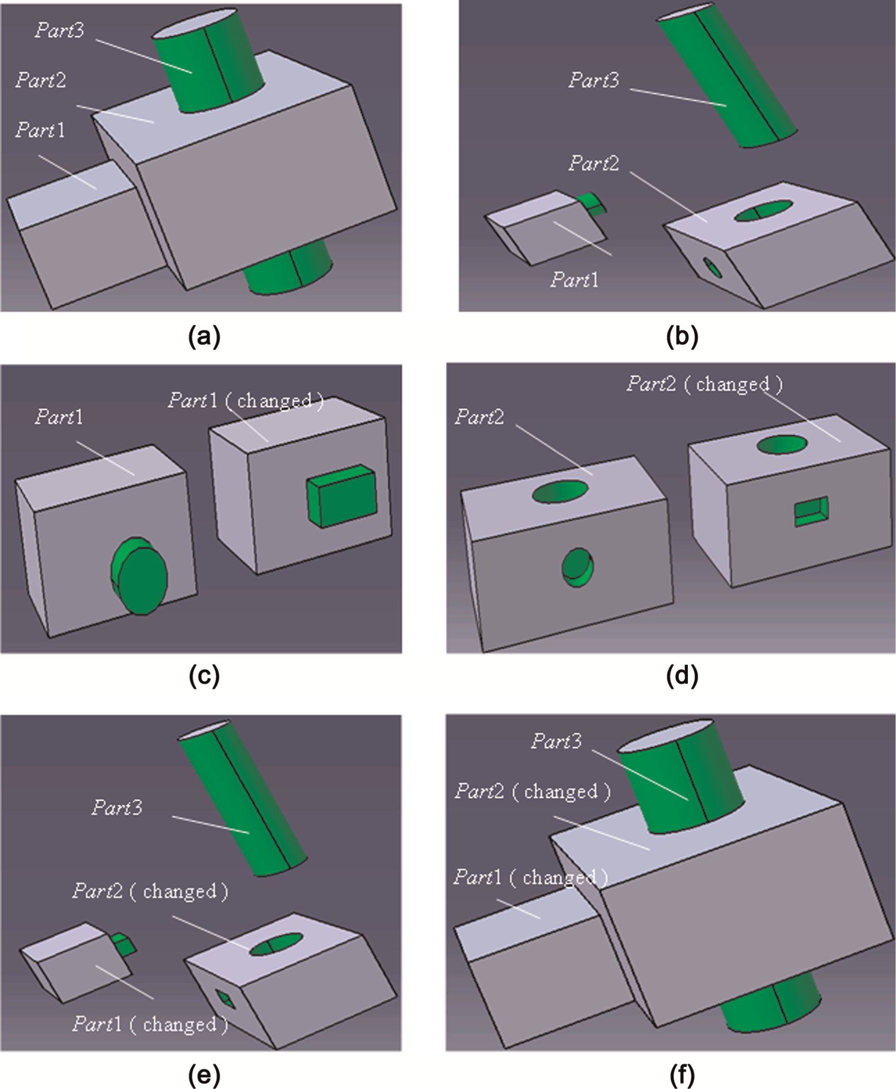
Instance of change in assembly tooling: (a) a simplified assembly tooling, (b) an exploded view of this assembly tooling, (c) a body with a cylinder boss is changed into a body with a cuboid boss, (d) a body with a cylinder groove is changed into a body with a cuboid groove, (e) an exploded view of the changed assembly tooling and (f) a new assembly tooling.

Figure 2.

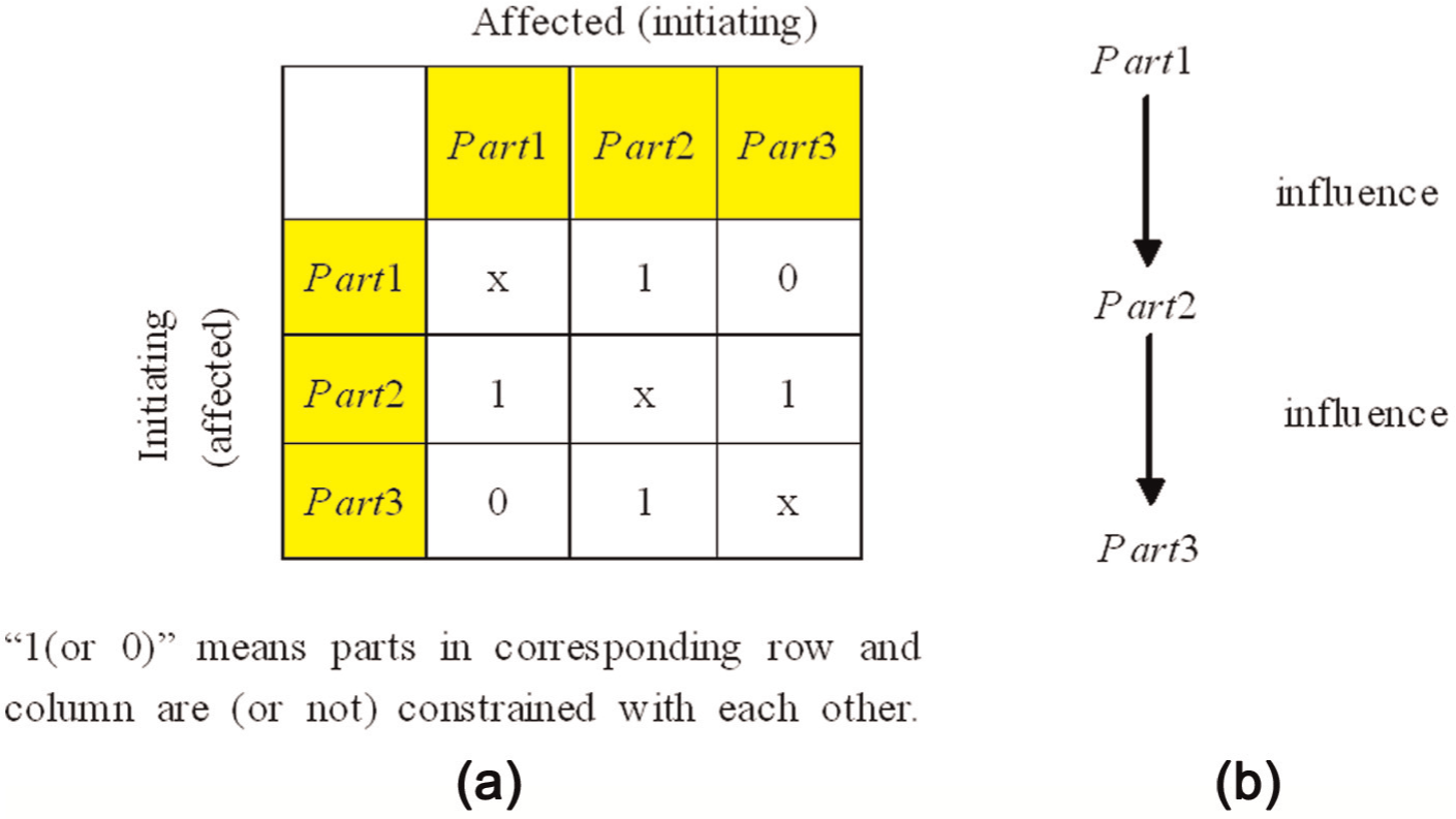
Change propagation case of assembly tooling: (a) DSM (at the part level) of the assembly tooling and (b) a false change propagation path of the assembly tooling.

To conclude, a majority of current DSM-based EC researches are conducted at the part or component level, which cannot provide more details of how changes propagate from one component to another and may lead to false change propagations. Accordingly, in this article, the geometrical relationships between parts or components are refined into the relationships between topology elements, that is, topology faces. The relationships between topology faces provide the rationales for change propagation. Furthermore, the relationships between topology faces are captured automatically from the computer-aided design (CAD) model, rather than acquired manually by designers with experiences.

Basic topology objects

In concurrent design, semantic feature model can be applied for integration of different domains. ¹⁹ Meanwhile, features can be represented by topological objects, which can be used to describe the geometrical information of components precisely and completely^20–25 by detailing their boundaries and connections, for example, faces or edges. ²⁶ Topology optimization in computer-aided mechanical part design is provided by Lu and Chen. ²⁷ And the method for integration of the topology and shape optimization into the design process is discussed by Spath et al. ²⁸ Normally, topology for geometrical design includes three types of entities, as shown in Table 1.

Table 1.

Basic topology objects.

Entity name	Entity definition	Entity description
Cell	A connected limitation of an underlying geometry	Most basic topological entity
Domain	A set of cells of dimension n connected by cells of dimension n − 1	Set of connected cells grouped to define boundaries
Body	A set of domains necessarily connected	A concrete object

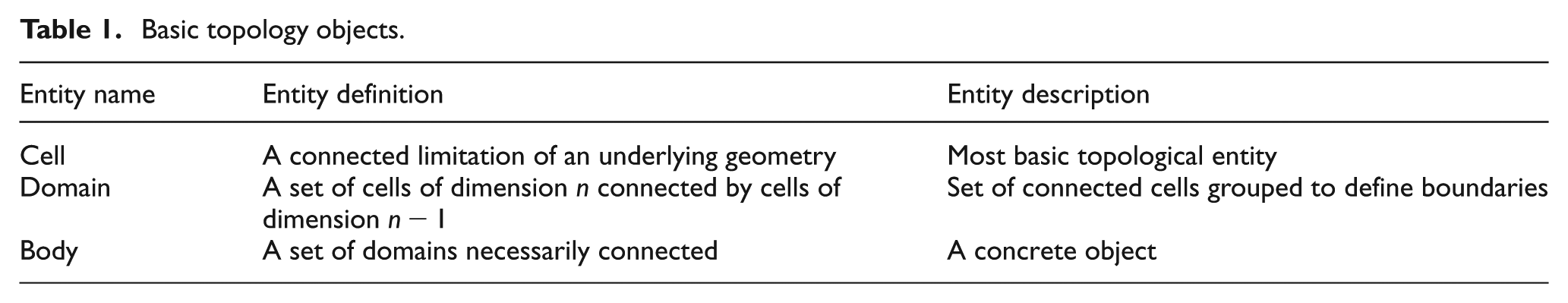
The cell is a connected limitation of an underlying geometry. In terms of the dimension in space they are in, cells are categorized into four types, that is, vertex, edge, face and volume. The cell type’s information is shown in Table 2 accordingly. Cells of upper dimensions are bounded by cells of lower dimensions, for example, a volume is the limitation of three-dimensional (3D) space by faces, and a face is the limitation of a surface by edges. A domain is a set of cells of dimension n connected by cells of dimension n − 1. And detailed examples are shown in Table 3.

Table 2.

Cell types.

Space dimension	Cell type	Associated geometry
0	Vertex	Point
1	Edge	Curve
2	Face	Surface
3	Volume	3D space

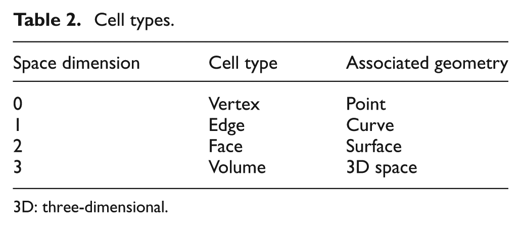
3D: three-dimensional.

Table 3.

Domain usage examples.

Domain entity	Composition of domain entity	Bounding entity
Loop	Edges connected by vertices	A face
Lump	Volumes connectedby faces	The 3D space
Shell	Faces connectedby edges	The 3D space or a volume
Wire	Edges connected by vertices	The 3D space

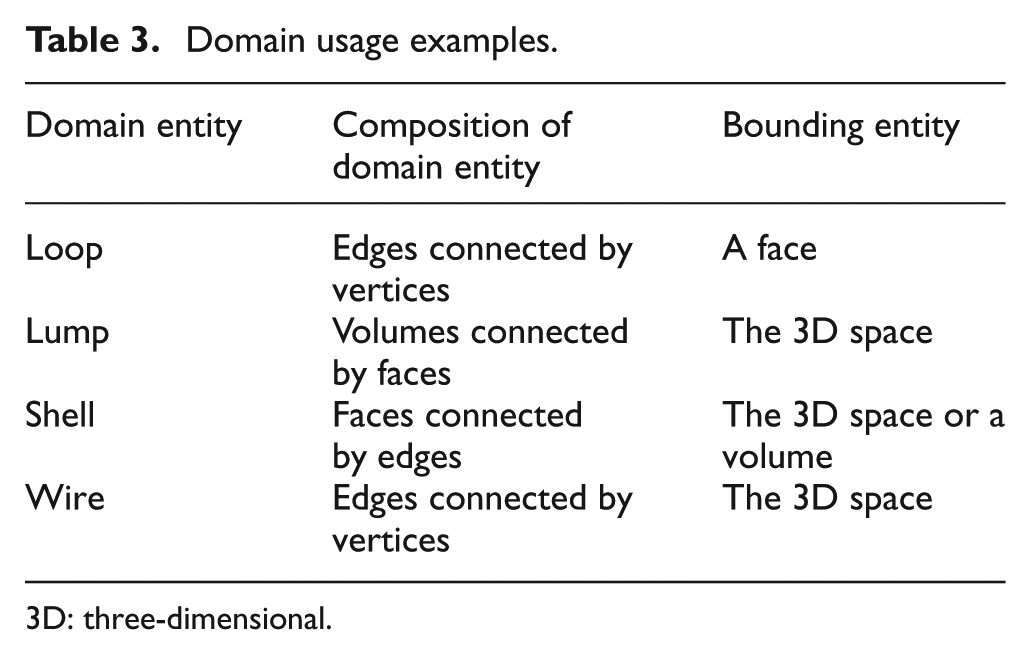
3D: three-dimensional.

Body is actually a set of domains connected and a part can be regarded as a body. For example, there is a part shown in Figure 3, which is composed of a lump made of one volume, that is, an entity. The volume has two shell boundaries: an inner shell and an outer shell. Outer shell is made up of six faces and inner shell is made up of only one face. In the outer shell, four faces are bounded by a loop and two faces are bounded by two loops. In the inner shell, only one face is bounded by two loops.

Figure 3.

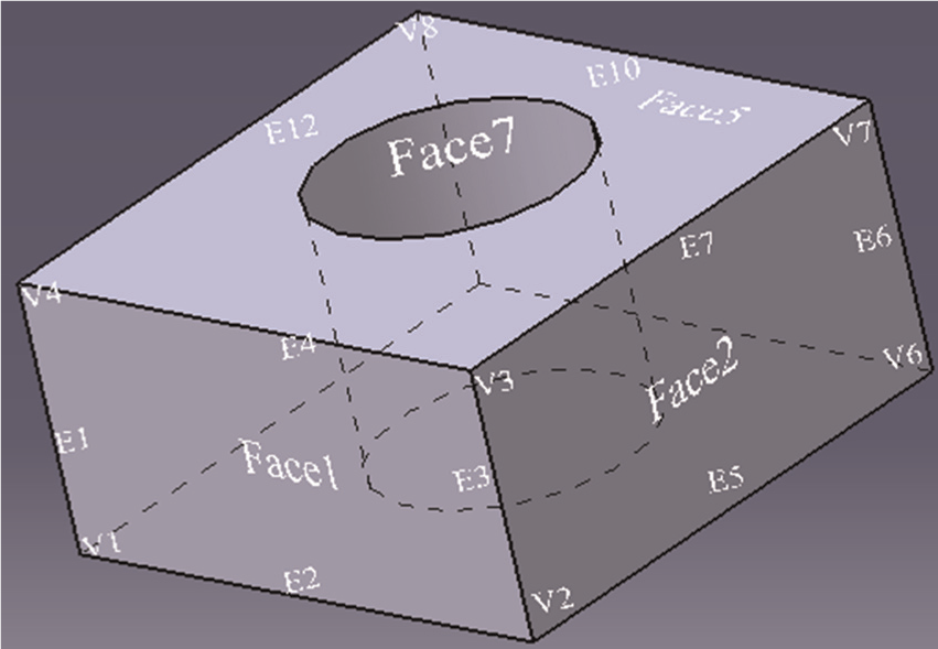
Basic topological objects.

In assembly tooling design, part as a 3D model can be bounded by topology faces. Topology face can be defined as the limitation of a surface by edges, which may be curved face or plane face. In this article, the smallest unit of a part model is topology face. A graph for the part decomposed into cells is shown in Figure 4 and it is called part decomposition graph (PDG). In Figure 4, control points (CPs) represent a number of points’ 3D coordinates acquired from the corresponding face. Besides, there is a one-to-one correspondence between a face and its corresponding CPs. Thus, a topology face is changed or not can be transformed into verifying whether its CPs remain as the same or not.

Figure 4.

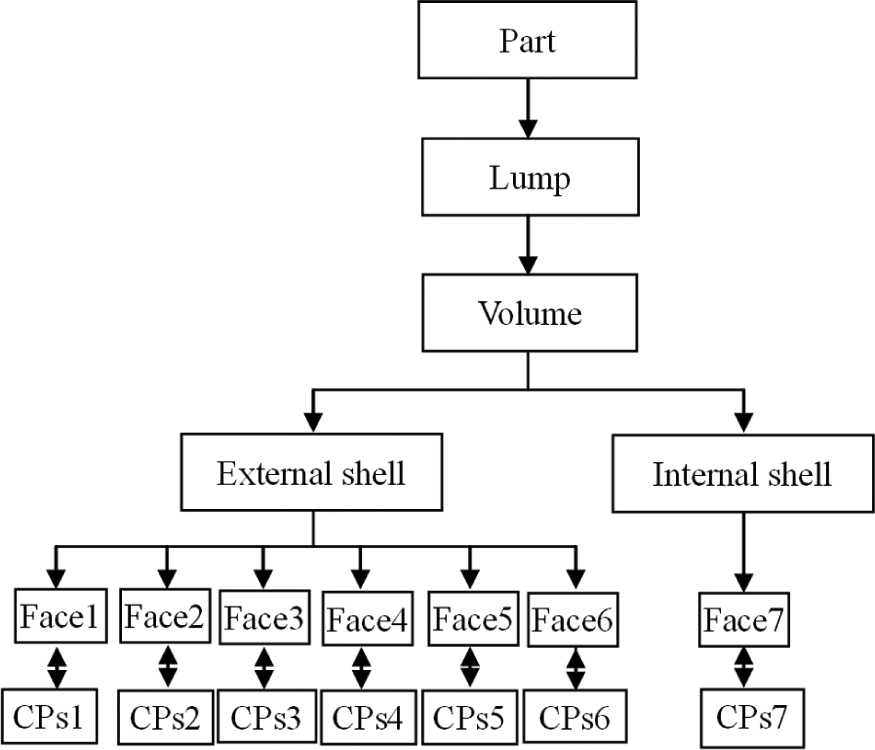
Part decomposition graph (PDG).

Constraint model

In assembly tooling design, part as a 3D model can be bounded by topology faces. And the topology faces of a part are represented in equation (1)

$$T(Parti)=\{F_i{}_1,F_i{}_2,\dots ,F_{ik},\dots ,F_{in}\}$$

(1)

where T(Part i) represents a set of topology faces of Part i. F_ik is one of the topology faces of Part i. n is the number of topology faces.

Geometrical constraints represent spatial relationships between components. ²⁹ To describe the change relationship between aircraft and its assembly tooling, a constraint model is proposed as shown in equation (2)

$$\begin{array}{c}\multicolumn{1}{c}{\mathrm{Re}(\mathrm{Part}i,\mathrm{Part}j)=\{F_{i1}\to F_{j1},F_{i2}\to F_{j2},\dots ,F_{\mathrm{ik}}}\\ \multicolumn{1}{c}{\to F_{\mathrm{jk}},\dots ,F_{\mathrm{im}}\to F_{\mathrm{jm}}\}}\end{array}$$

(2)

where Re(Part i, Part j) is a set of constraint relationships between topology faces from Part i and Part j. F_ik and F_jk are topology faces from Part i and Part j, respectively. F_ik→F_jk represents that F_jk is designed according to F_ik. m is the number of constraint relationships.

In Figure 5, 173Axxx is an aircraft and GZ-xxx AJ1 is its assembly tooling. The model is decomposed into four layers: product layer, subassembly layer, part layer and topology face layer. Besides, a product can consist of subassemblies and parts. A subassembly may consist of two parts or more. Parts are bounded by topology faces, and they can be constrained with each other through the topology face linkages. According to Figure 5, the one-way arrow means the arrow end part is designed according to the arrow start part and the double-headed arrow means that the dependence between the two parts is mutual. Aircraft design determines assembly tooling design, so the one-way arrows represent the relationships between the topology faces of an aircraft part and an assembly tooling part. The double-headed arrows represent the relationships between topology faces of aircraft parts (or assembly tooling parts). For example, Part3 of the 173Axxx is constrained by Part10 of the GZ-xxx AJ1 through the constraint between topology faces F₃₂ and F_101. The corresponding constraint model is shown in equation (3). Part6 of the 173Axxx is constrained by Part7 of the GZ-xxx AJ1 through the constraint between topology faces F₆₂ and F₇₁, and the corresponding constraint model is shown in equation (4). In conclusion, through mutual constraints by topology faces of parts, all the parts fit together to form the aircraft and assembly tooling

$$\mathrm{Re}(\mathrm{Part}3,\mathrm{Part}10)=\{F_{32}\to F_{101}\}$$

(3)

$$\mathrm{Re}(\mathrm{Part}6,\mathrm{Part}7)=\{F_{62}\to F_{71}\}$$

(4)

Figure 5.

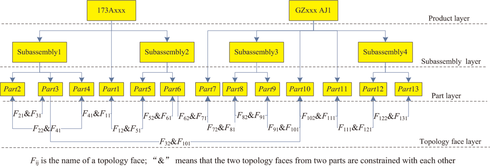
Relationship model of an aircraft and an assembly tooling.

Based on the constraint model, the relationship between two parts can be refined into the relationships between topology faces, and the change propagation can be analyzed through the linkages between topology faces. For example, a single change propagation path initiating from Part3 of 173Axxx to Part10, Part11 and Part13 of GZ-xxx AJ1 is demonstrated in Figure 6. First, a planned change is applied on the topology face F₃₂ of Part3. Due to the constraint between F₃₂ and F₁₀₁, F₁₀₁ of Part10 is influenced, which leads Part10 to change. After that, F₁₀₁ and F₁₀₂ having the same edge are adjacent, so F₁₀₂ is influenced too. Due to the linkage between F₁₀₂ and F₁₁₁, F₁₁₁ of Part11 is affected, leading Part11 to change. Finally, linkage between F₁₁₁ of Part11 and F₁₃₁ of Part13 leads Part13 to change. In this way, changes are propagated from aircraft parts to assembly tooling parts and spread between assembly tooling parts through topology faces.

Figure 6.

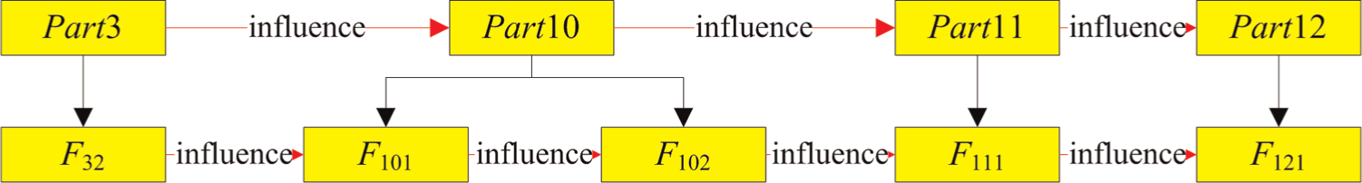
Change propagation path based on the topology face linkages.

Change propagation analysis method

In this article, a concept of change vector (CV) is presented to describe the change state of topology faces, and a concept of relation matrix (RM) is presented to describe the relationships between topology faces. Section “Change vector for aircraft part” illustrates how to capture an aircraft part CV and section “Relation matrix” details how to capture RM. In section “Change vector for assembly tooling part,” the change propagation from aircraft parts to assembly tooling parts is demonstrated based on CVs and RMs.

CV for aircraft part

The first step of the change propagation process is to capture CVs of the aircraft parts. CVs record the change state values of topology faces, and a general expression of a CV is shown in equation (5)

$$\mathrm{CV}(M)=(\begin{array}{ccccccc}\hfill a_1,\hfill & \hfill a_2,\hfill & \hfill \dots ,\hfill & \hfill a_i,\hfill & \hfill \dots \hfill & \hfill a_{n-1},\hfill & \hfill a_n\hfill \end{array})$$

(5)

where M is the name of an aircraft part. a_i is the change state value of the ith topology face. n is the number of topology faces of part M. a_i can be valued as 1 or 0. 1 (or 0) means the corresponding topology face is changed (or unchanged).

For example, a cuboid is changed from (a) to (b) as shown in Figure 7, that is, Face2 is changed from a plane face to a curved face. Due to the common edges with Face2, the adjacent faces Face1, Face3, Face5 and Face6 are also changed. Thus, the CV is (1, 1, 1, 0, 1, 1, 0).

Figure 7.

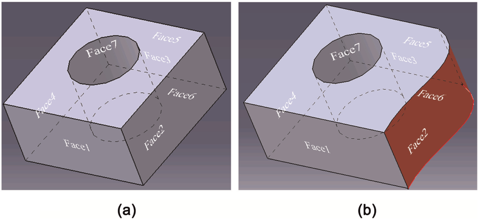
Example of change in topology face: (a) a part and (b) Face2 is changed along with Face1, Face3, Face5 and Face6.

According to the PDG in Figure 4, a part corresponds to a number of topology faces and a topology face corresponds to a number of CPs. The information of topology faces and corresponding CPs can be captured from the CAD model and recorded in a database. The flowchart of capturing CV is shown in Figure 8. CPs are used to verify whether a topology face is changed or not in the process. Details are as follows:

• Step 1: The sequence number k of an original aircraft part is initially set to 1.

• Step 2: Acquiring the topology faces’ CPs of original aircraft part k.

• Step 3: An iteration process is implemented to identify whether the CPs of original aircraft part k have been changed or not. Topology faces’ CPs of original aircraft part k are compared with those of changed aircraft parts (Part1, Part2,..., Part i,..., Part n). And CV of the aircraft part k is captured. After that, the part sequence number k is added by 1 (k = k + 1).

• Step 4: If $k\le m$ , go to Step 2; otherwise go to Step 5.

• Step 5: End of program.

Figure 8.

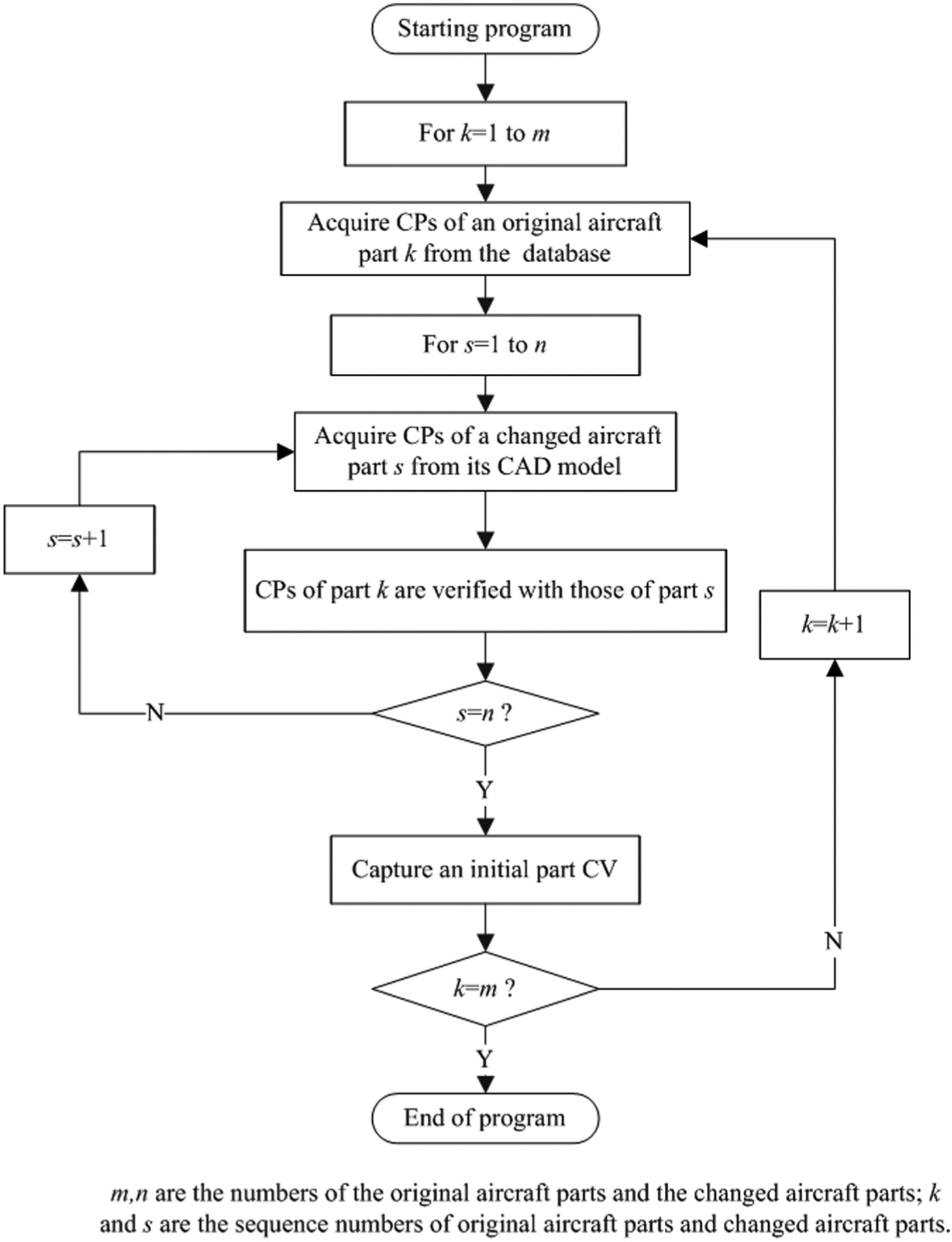
Flowchart of capturing change vector of aircraft part.

RM

In the aircraft-assembly tooling design, changes in aircraft parts will influence assembly tooling parts, and a changed assembly tooling part may influence other assembly tooling parts.

Edwin et al., ¹⁵ Giffin et al. ¹⁶ and Keller et al. ¹⁷ use a DSM-based approach to study change propagation. However, values of the matrix are captured manually by domain experts, which is time-consuming and effort-consuming. In this article, RMs (at the topology face level) are captured automatically from the original CAD model with developed algorithms. The types of RM and the algorithms of capturing RM are detailed in this section.

Type of RM

Due to the relationships between the topology faces of aircraft parts and assembly tooling parts, RM is divided into three types.

Type1: Aircraft-assembly tooling RM

This type of RM is to depict the relationships between topology faces of an aircraft part and an assembly tooling part. It is a semi-matrix which means that the topology faces of part N can be influenced by the topology faces of part M, and it is formulated in equation (6)

$$\mathrm{RM}(M,N)=\left(\begin{array}{c}\hfill a_{1n}\hfill \\ \multicolumn{1}{c}{⋮}\\ \multicolumn{1}{c}{a_{i1}}\\ \multicolumn{1}{c}{⋮}\\ \multicolumn{1}{c}{a_{m1}}\end{array}\begin{array}{c}\hfill \dots \hfill \\ \multicolumn{1}{c}{}\\ \multicolumn{1}{c}{\dots }\\ \multicolumn{1}{c}{}\\ \multicolumn{1}{c}{\dots }\end{array}\begin{array}{c}\hfill a_{1j}\hfill \\ \multicolumn{1}{c}{\ddots }\\ \multicolumn{1}{c}{a_{\mathrm{ij}}}\\ \multicolumn{1}{c}{\ddots }\\ \multicolumn{1}{c}{a_{\mathrm{mj}}}\end{array}\begin{array}{c}\hfill \dots \hfill \\ \multicolumn{1}{c}{}\\ \multicolumn{1}{c}{\dots }\\ \multicolumn{1}{c}{}\\ \multicolumn{1}{c}{\dots }\end{array}\begin{array}{c}\hfill a_{1n}\hfill \\ \multicolumn{1}{c}{⋮}\\ \multicolumn{1}{c}{a_{\mathrm{in}}}\\ \multicolumn{1}{c}{⋮}\\ \multicolumn{1}{c}{a_{\mathrm{mn}}}\end{array}\right)$$

(6)

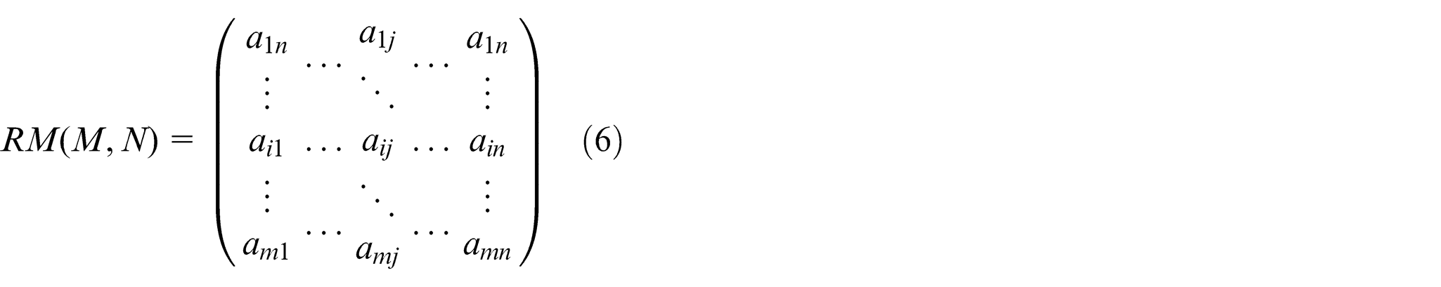
where M and N are the names of an aircraft part and an assembly tooling part, respectively. a_ij represents the change relationship between the ith topology face of Part M and the jth topology face of Part N. m and n are the numbers of topology faces of part M and part N, respectively. a_ij can be valued as 1 or 0. The value 1 (or 0) means that the two topology faces from two parts are (or are not) constrained with each other.

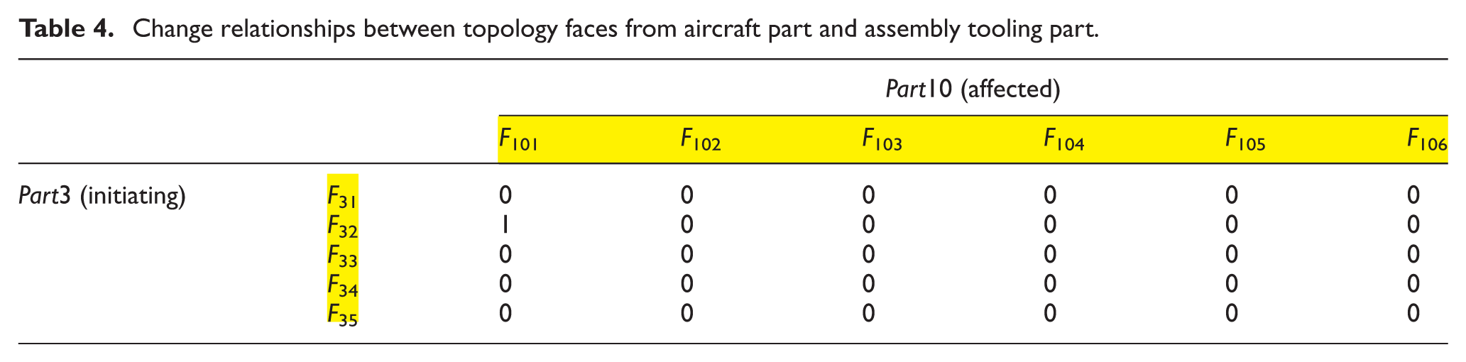
The relationship model in Figure 5 is used to demonstrate the process of capturing the aircraft-assembly tooling RM. As shown in Figure 5, Part1, Part 2, Part3, Part4, Part5 and Part6 belong to the aircraft. The others belong to the assembly tooling. Constraints exist between F₃₂ of Part3 and F₁₀₁ of Part10 and F₆₂ of Part6 and F₇₁ of Part7. And the change relationships between the topology faces of Part3 and Part10 are used to demonstrate the RM. It is assumed that Part3 has five topology faces named F₃₁, F₃₂, F₃₃, F₃₄ and F₃₅, and Part10 has six topology faces named F₁₀₁, F₁₀₂, F₁₀₃, F₁₀₄, F₁₀₅ and F₁₀₆. There is a constraint between F₃₂ and F₁₀₁, so the value for the change relationship is 1. The others are 0. Accordingly, a change relationship matrix is constructed in Table 4, and RM (Part3, Part10) is shown in equation (7)

$$\mathrm{RM}(\mathrm{Part}3,P\mathrm{art}10)=\left(\begin{array}{cccccc}\hfill 0\hfill & \hfill 0\hfill & \hfill 0\hfill & \hfill 0\hfill & \hfill 0\hfill & \hfill 0\hfill \\ \multicolumn{1}{c}{1}& \hfill 0\hfill & \hfill 0\hfill & \hfill 0\hfill & \hfill 0\hfill & \hfill 0\hfill \\ \multicolumn{1}{c}{0}& \hfill 0\hfill & \hfill 0\hfill & \hfill 0\hfill & \hfill 0\hfill & \hfill 0\hfill \\ \multicolumn{1}{c}{0}& \hfill 0\hfill & \hfill 0\hfill & \hfill 0\hfill & \hfill 0\hfill & \hfill 0\hfill \\ \multicolumn{1}{c}{0}& \hfill 0\hfill & \hfill 0\hfill & \hfill 0\hfill & \hfill 0\hfill & \hfill 0\hfill \end{array}\right)$$

(7)

Table 4.

Change relationships between topology faces from aircraft part and assembly tooling part.

		Part10 (affected)
		F 101	F 102	F 103	F 104	F 105	F 106
Part3 (initiating)	F 31	0	0	0	0	0	0
	F 32	1	0	0	0	0	0
	F 33	0	0	0	0	0	0
	F 34	0	0	0	0	0	0
	F 35	0	0	0	0	0	0

Type2: Assembly tooling part RM

This type of RM is to depict the change relationships between topology faces of an assembly tooling part. In this article, we assume that topology faces having common edges have change relationships with each other. Besides, a general name for this type of matrix is RM (M). It is a symmetric matrix, and the expression is shown in equation (8)

$$\mathrm{RM}(M)=\left(\begin{array}{c}\hfill a_{1n}\hfill \\ \multicolumn{1}{c}{⋮}\\ \multicolumn{1}{c}{a_{i1}}\\ \multicolumn{1}{c}{⋮}\\ \multicolumn{1}{c}{a_{n1}}\end{array}\begin{array}{c}\hfill \dots \hfill \\ \multicolumn{1}{c}{}\\ \multicolumn{1}{c}{\dots }\\ \multicolumn{1}{c}{}\\ \multicolumn{1}{c}{\dots }\end{array}\begin{array}{c}\hfill a_{1j}\hfill \\ \multicolumn{1}{c}{\ddots }\\ \multicolumn{1}{c}{a_{\mathrm{ij}}}\\ \multicolumn{1}{c}{\ddots }\\ \multicolumn{1}{c}{a_{\mathrm{nj}}}\end{array}\begin{array}{c}\hfill \dots \hfill \\ \multicolumn{1}{c}{}\\ \multicolumn{1}{c}{\dots }\\ \multicolumn{1}{c}{}\\ \multicolumn{1}{c}{\dots }\end{array}\begin{array}{c}\hfill a_{1n}\hfill \\ \multicolumn{1}{c}{⋮}\\ \multicolumn{1}{c}{a_{\mathrm{in}}}\\ \multicolumn{1}{c}{⋮}\\ \multicolumn{1}{c}{a_{\mathrm{nn}}}\end{array}\right)$$

(8)

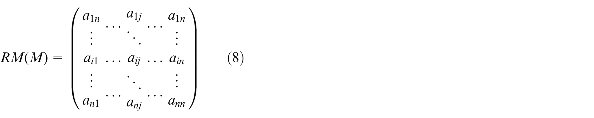
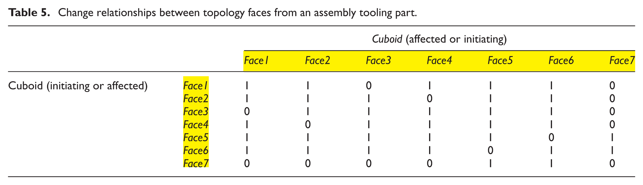
where M is the name of an assembly tooling part. a_ij represents the change relationship between the ith topology face and the jth topology face of Part M. n is the quantity of topology faces of part M. a_ij can be valued as 1 or 0. 1 (or 0) means that the two topology faces from the part have (or have no) common edges with each other. For example, a RM to describe the relationships between topology faces from the Cuboid in Figure 7(a) is shown in Table 5, and RM (Cuboid) is shown in equation (9)

$$\mathrm{RM}(\mathrm{Cuboid})=\left(\begin{array}{ccccccc}\hfill 1\hfill & \hfill 1\hfill & \hfill 0\hfill & \hfill 1\hfill & \hfill 1\hfill & \hfill 1\hfill & \hfill 0\hfill \\ \multicolumn{1}{c}{1}& \hfill 1\hfill & \hfill 1\hfill & \hfill 0\hfill & \hfill 1\hfill & \hfill 1\hfill & \hfill 0\hfill \\ \multicolumn{1}{c}{0}& \hfill 1\hfill & \hfill 1\hfill & \hfill 1\hfill & \hfill 1\hfill & \hfill 1\hfill & \hfill 0\hfill \\ \multicolumn{1}{c}{1}& \hfill 0\hfill & \hfill 1\hfill & \hfill 1\hfill & \hfill 1\hfill & \hfill 1\hfill & \hfill 0\hfill \\ \multicolumn{1}{c}{1}& \hfill 1\hfill & \hfill 1\hfill & \hfill 1\hfill & \hfill 1\hfill & \hfill 0\hfill & \hfill 1\hfill \\ \multicolumn{1}{c}{1}& \hfill 1\hfill & \hfill 1\hfill & \hfill 1\hfill & \hfill 0\hfill & \hfill 1\hfill & \hfill 1\hfill \\ \multicolumn{1}{c}{0}& \hfill 0\hfill & \hfill 0\hfill & \hfill 0\hfill & \hfill 1\hfill & \hfill 1\hfill & \hfill 0\hfill \end{array}\right)$$

(9)

Table 5.

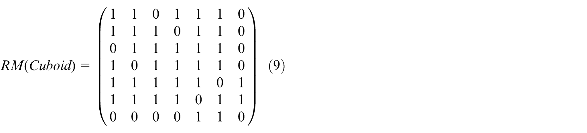
Change relationships between topology faces from an assembly tooling part.

		Cuboid (affected or initiating)
		Face1	Face2	Face3	Face4	Face5	Face6	Face7
Cuboid (initiating or affected)	Face1	1	1	0	1	1	1	0
	Face2	1	1	1	0	1	1	0
	Face3	0	1	1	1	1	1	0
	Face4	1	0	1	1	1	1	0
	Face5	1	1	1	1	1	0	1
	Face6	1	1	1	1	0	1	1
	Face7	0	0	0	0	1	1	0

Type3: Assembly tooling–assembly tooling RM

This type of RM is to depict the change relationships between the topology faces of two assembly tooling parts. The representation is similar to that of Type1. It should be noted that the topology faces captured for the RM of Type1 and Type3 are different in influence direction. The influence direction of RM of Type1 is from the topology faces of aircraft parts to those of the assembly tooling parts, but for the RM of Type3, the influence is mutual due to the design philosophy. The assembly tooling–assembly tooling RM expression is shown in equation (10)

$$\mathrm{RM}\prime (M,N)=\left(\begin{array}{c}\hfill a_{1n}\hfill \\ \multicolumn{1}{c}{⋮}\\ \multicolumn{1}{c}{a_{i1}}\\ \multicolumn{1}{c}{⋮}\\ \multicolumn{1}{c}{a_{m1}}\end{array}\begin{array}{c}\hfill \dots \hfill \\ \multicolumn{1}{c}{}\\ \multicolumn{1}{c}{\dots }\\ \multicolumn{1}{c}{}\\ \multicolumn{1}{c}{\dots }\end{array}\begin{array}{c}\hfill a_{1j}\hfill \\ \multicolumn{1}{c}{\ddots }\\ \multicolumn{1}{c}{a_{\mathrm{ij}}}\\ \multicolumn{1}{c}{\ddots }\\ \multicolumn{1}{c}{a_{\mathrm{mj}}}\end{array}\begin{array}{c}\hfill \dots \hfill \\ \multicolumn{1}{c}{}\\ \multicolumn{1}{c}{\dots }\\ \multicolumn{1}{c}{}\\ \multicolumn{1}{c}{\dots }\end{array}\begin{array}{c}\hfill a_{1n}\hfill \\ \multicolumn{1}{c}{⋮}\\ \multicolumn{1}{c}{a_{\mathrm{in}}}\\ \multicolumn{1}{c}{⋮}\\ \multicolumn{1}{c}{a_{\mathrm{mn}}}\end{array}\right)$$

(10)

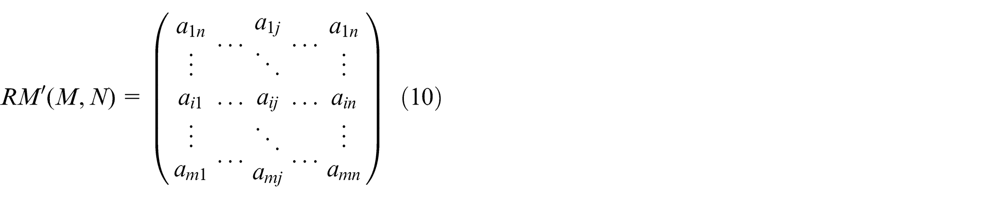
where M and N are the names of the two assembly tooling parts. a_ij represents the change relationship between the ith topology face of part M and the jth topology face of part N. m and n are the numbers of topology faces from part M and N. a_ij can be valued as 1 or 0. The value 1 (or 0) means that two topology faces from the two assembly tooling parts are (or are not) constrained with each other.

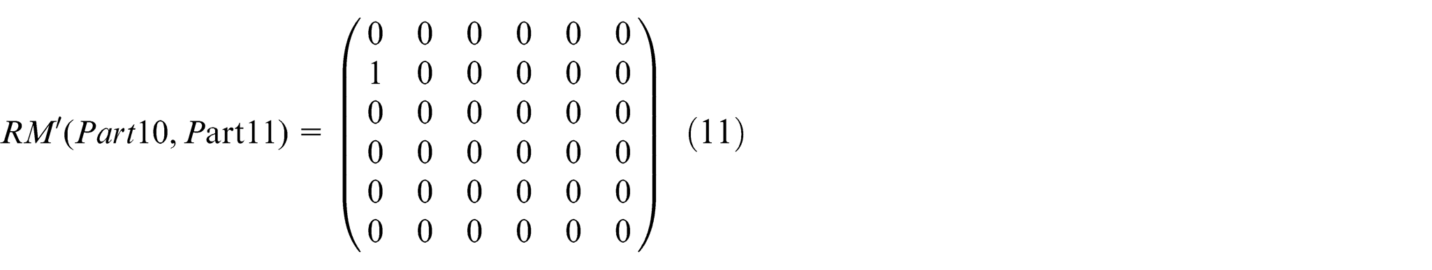
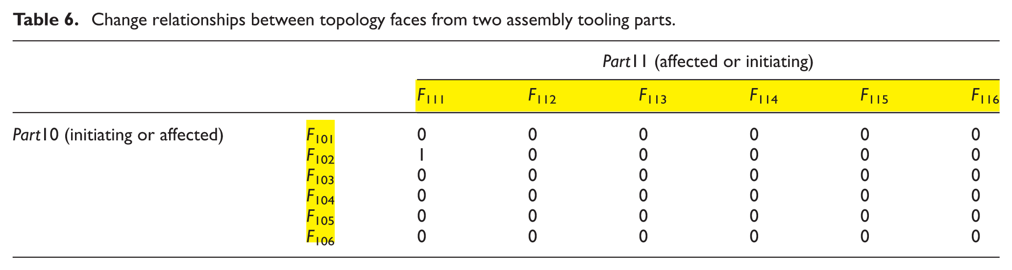
Change relationships between topology faces of Part10 and Part11 in Figure 5 are taken as examples. We assume that the quantity of topology faces of Part11 is the same as that of topology faces of Part10. And F₁₀₂ and F₁₁₁ are constrained with each other. A RM is constructed in Table 6 and RM′ (Part10, Part11) is shown in equation (11)

$$\mathrm{RM}\prime (\mathrm{Part}10,P\mathrm{art}11)=\left(\begin{array}{cccccc}\hfill 0\hfill & \hfill 0\hfill & \hfill 0\hfill & \hfill 0\hfill & \hfill 0\hfill & \hfill 0\hfill \\ \multicolumn{1}{c}{1}& \hfill 0\hfill & \hfill 0\hfill & \hfill 0\hfill & \hfill 0\hfill & \hfill 0\hfill \\ \multicolumn{1}{c}{0}& \hfill 0\hfill & \hfill 0\hfill & \hfill 0\hfill & \hfill 0\hfill & \hfill 0\hfill \\ \multicolumn{1}{c}{0}& \hfill 0\hfill & \hfill 0\hfill & \hfill 0\hfill & \hfill 0\hfill & \hfill 0\hfill \\ \multicolumn{1}{c}{0}& \hfill 0\hfill & \hfill 0\hfill & \hfill 0\hfill & \hfill 0\hfill & \hfill 0\hfill \\ \multicolumn{1}{c}{0}& \hfill 0\hfill & \hfill 0\hfill & \hfill 0\hfill & \hfill 0\hfill & \hfill 0\hfill \end{array}\right)$$

(11)

Table 6.

Change relationships between topology faces from two assembly tooling parts.

		Part11 (affected or initiating)
		F 111	F 112	F 113	F 114	F 115	F 116
Part10 (initiating or affected)	F 101	0	0	0	0	0	0
	F 102	1	0	0	0	0	0
	F 103	0	0	0	0	0	0
	F 104	0	0	0	0	0	0
	F 105	0	0	0	0	0	0
	F 106	0	0	0	0	0	0

Algorithm to capture RM

In the algorithm, CPs are used to identify the two topology faces which have change relationship with each other. There are three types of RMs captured. The algorithm of capturing RMs of Type1 and Type3 is the same and the algorithm of capturing RM of Type2 is a little different.

• 1. Algorithm of capturing RMs of Type1 and Type3.

• Change relationships between topology faces can be captured from the constraint interfaces of the CAD model of aircraft and assembly tooling. A flowchart in Figure 9 is to show the process of capturing RM. Detailed steps are illustrated as follows:

• Step 1: Relationships between a part and corresponding topology faces and relationships between topology faces and corresponding CPs are stored in a database.

• Step 2: The constraint interfaces of the CAD model of aircraft and assembly tooling are acquired. Through the relationships in the interfaces, CPs of the topology faces constrained with each other are captured.

• Step 3: CPs acquired in Step 2 are verified with CPs stored in the database.

• Step 4: If the CPs acquired in Step 2 are found in the database, corresponding topology faces are recognized and values for the change relationship in the RM are set to 1. Moreover, the corresponding parts’ names are also identified.

• Step 5: End of program.

Figure 9.

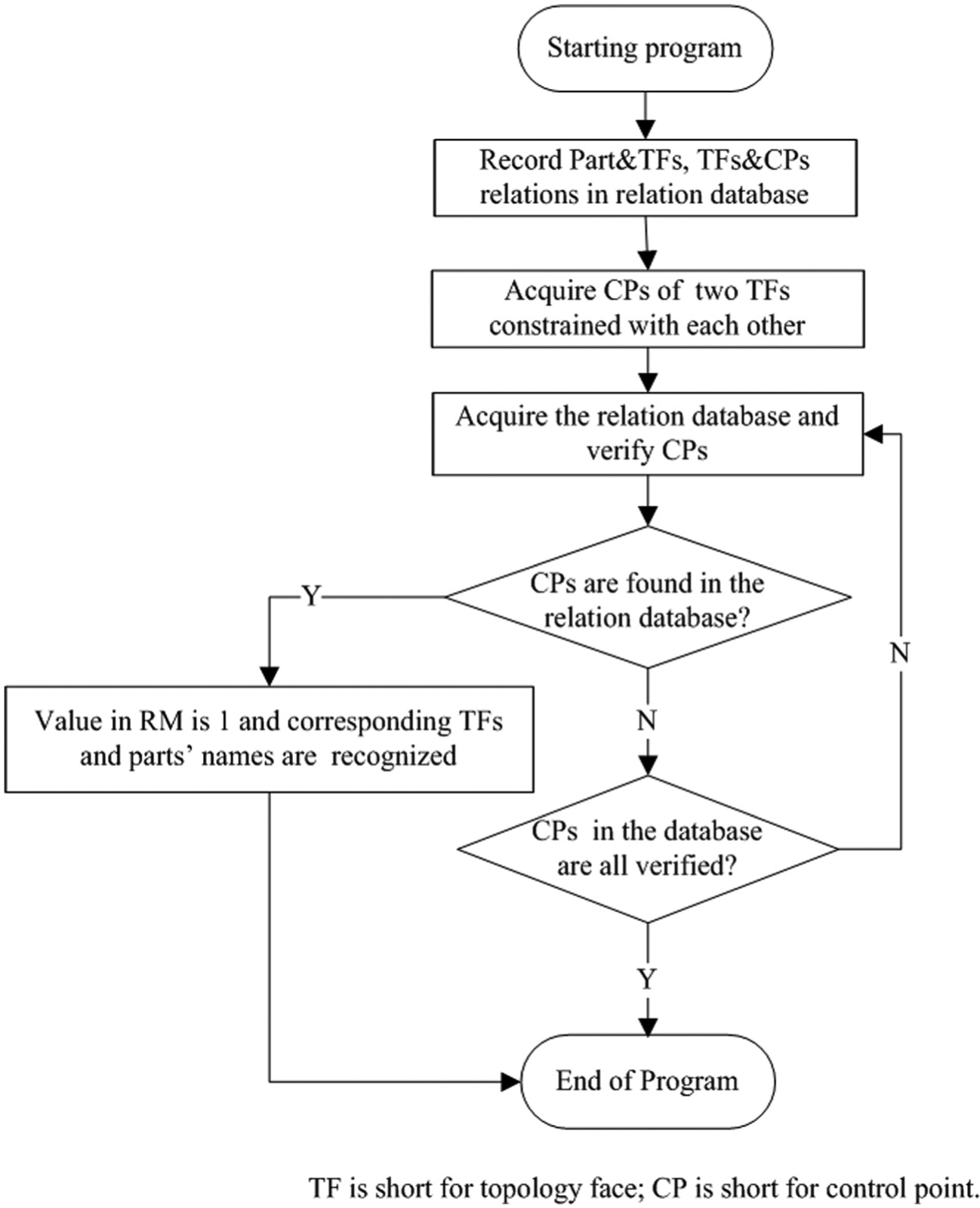
Flowchart of capturing RMs of Type1 and Type3.

Through the above steps, RMs are stored in a database for computation of the following change propagation.

• 2. Algorithm of capturing RM of Type2.

• RM of Type2 is captured through searching common edges between the topology faces of an assembly tooling part. A flowchart in Figure 10 is to describe the process of capturing RM. Detailed steps are as follows:

• Step 1: An assembly tooling part, its topology faces and corresponding CPs are stored in a database, whose structure is similar to that of the PDG.

• Step 2: The part’s topology faces are acquired.

• Step 3: Pairwise verification of topology faces is implemented to search topology faces having common edges.

• Step 4: If common edges are found between any two topology faces, value for the change relationship in the RM is set to 1. Moreover, the part’s name is also recognized.

• Step 5: End of program.

Figure 10.

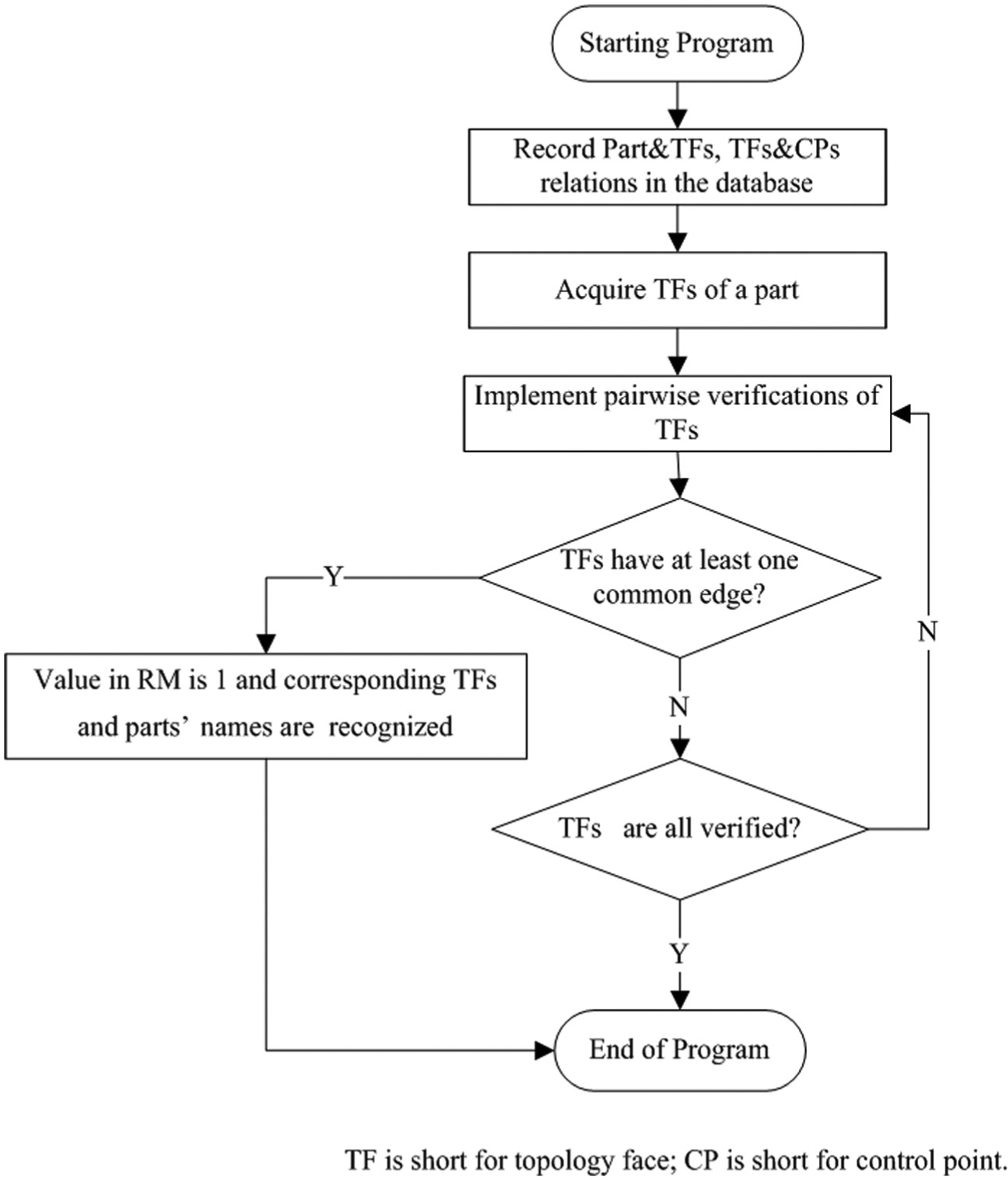
Flowchart of capturing RM of Type2.

Through the above steps, RMs are also stored in the database for computation of the following change propagation.

CV for assembly tooling part

Based on the above steps, an algorithm is proposed to compute the assembly tooling part CVs. First, initial changes are captured by verifying the topology faces of aircraft parts. Then, changes are propagated to the assembly tooling parts through linkages between the topology faces of aircraft parts and assembly tooling parts. After that, changes spread between assembly tooling parts through mutual constraints between topology faces of assembly tooling parts. Computationally, a general expression for this algorithm is shown in equation (12)

$$\mathrm{CV}(\mathrm{Ass}-k)=\{\begin{array}{cc}\hfill \mathrm{CV}(\mathrm{Air}-i)\mathrm{RM}(\mathrm{Air}-i,\mathrm{Ass}-1)\mathrm{RM}(\mathrm{Ass}-1)\hfill & \hfill k=1\hfill \\ \multicolumn{1}{c}{\mathrm{CV}(\mathrm{Ass}-1)\underset{j=2}{\overset{k}{\Pi }}\mathrm{RM}\prime (\mathrm{Ass}-j-1,\mathrm{Ass}-j)\mathrm{RM}(\mathrm{Ass}-j)}& \hfill 2\Leftarrow k\Leftarrow n\hfill \end{array}$$

(12)

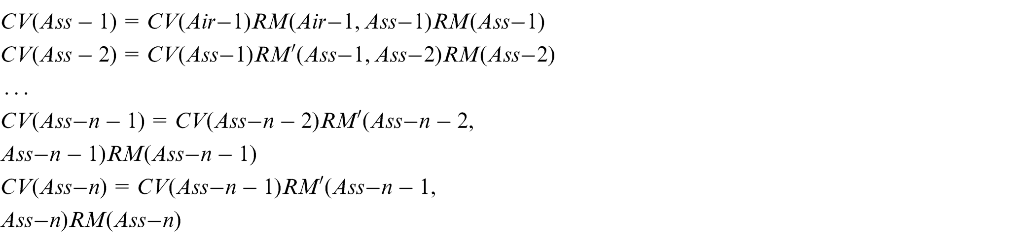
where i is the sequence number of changed aircraft part, ranging from 1 to m (m is the quantity of changed aircraft parts). k is the sequence number of influenced assembly tooling part along a single change propagation path, ranging from 1 to n (n is the quantity of influenced assembly tooling parts along the single change propagation path). n varies according to different change propagation paths. Air-i is the name of the ith changed aircraft part. Ass-j is the name of the jth influenced assembly tooling part along a single change propagation path.

A change propagation process is shown as follows. First, an aircraft part CV is captured. In the first change propagation step, the aircraft part CV is multiplied sequentially by an aircraft-assembly tooling RM and an assembly tooling part RM to obtain the first influenced part CV of the assembly tooling. In the second change propagation step, the first influenced part CV is multiplied sequentially by an assembly tooling–assembly tooling RM and an assembly tooling part RM. And the second influenced part CV of the assembly tooling is obtained. Then, computational processes similar to that in the second change propagation step is cycled until no assembly tooling parts are influenced. For example, we consider a single change propagation path of n steps, which has 1 aircraft part CV, n assembly tooling part CVs, 1 aircraft-assembly tooling RM, n assembly tooling part RMs and n − 1 assembly tooling–assembly tooling RMs. The computational process is shown below

$$\begin{array}{c}\multicolumn{1}{c}{\mathrm{CV}(\mathrm{Ass}-1)=\mathrm{CV}(\mathrm{Air}-1)\mathrm{RM}(\mathrm{Air}-1,\mathrm{Ass}-1)\mathrm{RM}(\mathrm{Ass}-1)}\\ \multicolumn{1}{c}{\mathrm{CV}(\mathrm{Ass}-2)=\mathrm{CV}(\mathrm{Ass}-1)\mathrm{RM}\prime (\mathrm{Ass}-1,\mathrm{Ass}-2)\mathrm{RM}(\mathrm{Ass}-2)}\\ \multicolumn{1}{c}{\dots }\\ \multicolumn{1}{c}{\mathrm{CV}(\mathrm{Ass}-n-1)=\mathrm{CV}(\mathrm{Ass}-n-2)\mathrm{RM}\prime (\mathrm{Ass}-n-2,}\\ \multicolumn{1}{c}{\mathrm{Ass}-n-1)\mathrm{RM}(\mathrm{Ass}-n-1)}\\ \multicolumn{1}{c}{\mathrm{CV}(\mathrm{Ass}-n)=\mathrm{CV}(\mathrm{Ass}-n-1)\mathrm{RM}\prime (\mathrm{Ass}-n-1,}\\ \multicolumn{1}{c}{\mathrm{Ass}-n)\mathrm{RM}(\mathrm{Ass}-n)}\end{array}$$

An assembly tooling part CV is shown in equation (13). And the summation of values in the CV is named CI index which is shown in equation (14). The larger the CI index, the more the part is influenced

$$\mathrm{CV}(M)=(\begin{array}{ccccccc}\hfill a_1,\hfill & \hfill a_2,\hfill & \hfill \dots ,\hfill & \hfill a_i,\hfill & \hfill \dots ,\hfill & \hfill a_{n-1},\hfill & \hfill a_n\hfill \end{array})$$

(13)

where M is the name of an assembly tooling part. a_i is the change state value of the ith topology face of part M. n is the quantity of topology faces from part M. a_i can be 0 or a nonzero natural number. The value 0 (or nonzero natural number) means the corresponding topology face is unaffected (or affected)

$$\mathrm{CI}(M)=\sum _{i=1}^n{a}_i$$

(14)

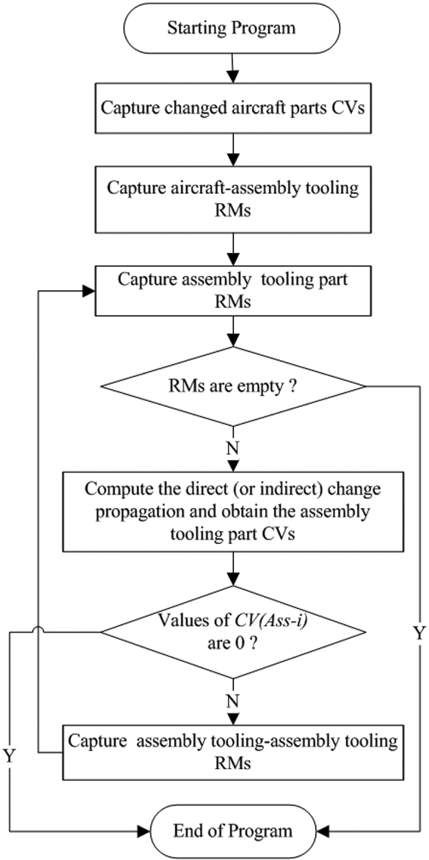
The flowchart of the change propagation analysis method is described in Figure 11. Detailed steps are as follows:

• Step 1: CVs of the changed aircraft parts are captured according to the algorithm in section “Change vector for aircraft part.”

• Step 2: Aircraft-assembly tooling RMs are captured according to the first algorithm in section “Algorithm to capture RM.”

• Step 3: Assembly tooling Part RMs are captured according to second algorithm in section “Algorithm to capture RM.”

•  If (RMs are empty)

•   Go to Step 6.

•  Else

•   Go to Step 4.

• Step 4: Assembly tooling parts’ CVs from the direct (or indirect) change propagation are computed according to the algorithm in section “Change vector for assembly tooling part.”

•  If (CVs = 0)

•   Go to Step 6.

•  Else

•   Go to Step 5.

• Step 5: Assembly tooling–assembly tooling RMs are captured according to the first algorithm in section “Algorithm to capture RM.”

•  If (RMs are empty)

•   Go to Step 6.

•  Else

•   Go to Step 3.

• Step 6: End of program.

Figure 11.

Flowchart of change propagation.

The judgments are used to determine whether the change propagation process should be finished. Values of CV equaling to 0 mean that the part’s topology faces remain unchanged and the change propagation process ends. Besides, if the RM is empty, which means the influenced part’s topology faces have no change relationships with the remaining topology faces of assembly tooling parts, the process also ends.

Case study

Based on the method and algorithms above, a computer-aided change propagation analysis system is developed with CATIA V5 using the CAA technology, including module of capturing CV for aircraft parts, module of capturing relation matrices, module of implementing change propagation and module of outputting change list.

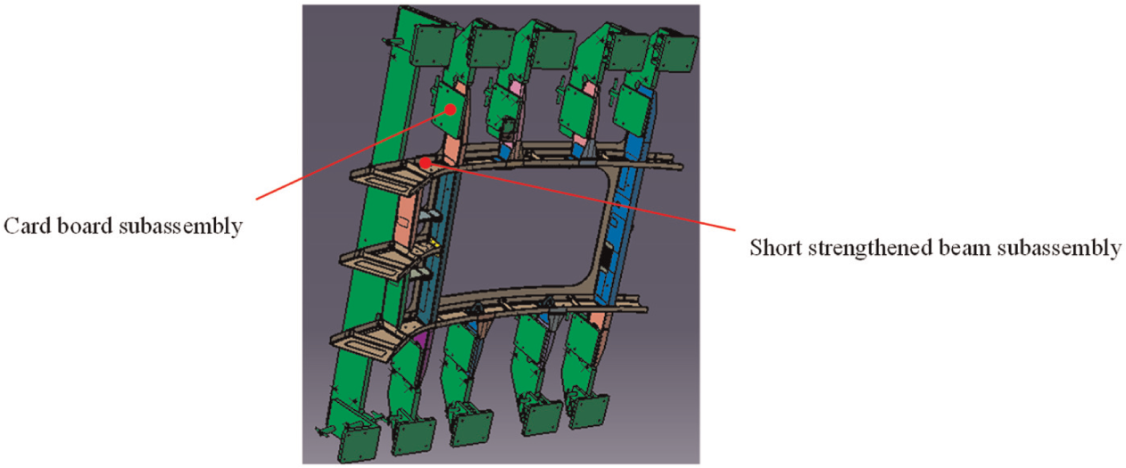
An assembly tooling called GZ-xxx AJ1 in Figure 12 is applied to test the system. The assembly tooling consists of a skeleton, a subassembly of cardboard and a subassembly of frame positioning, which are in blue, green and yellow sequentially. And the frame of an aircraft is also shown in Figure 12. The cardboard subassembly’s function is to locate the short strengthened beam subassembly of the frame as shown in Figure 13.

Figure 12.

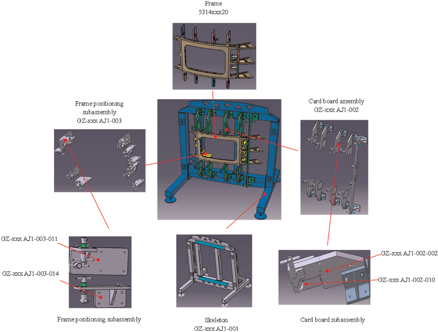
Application instance.

Figure 13.

Constraint relationship.

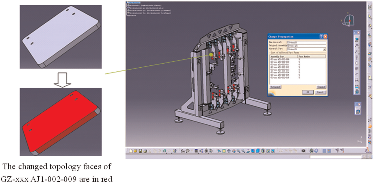
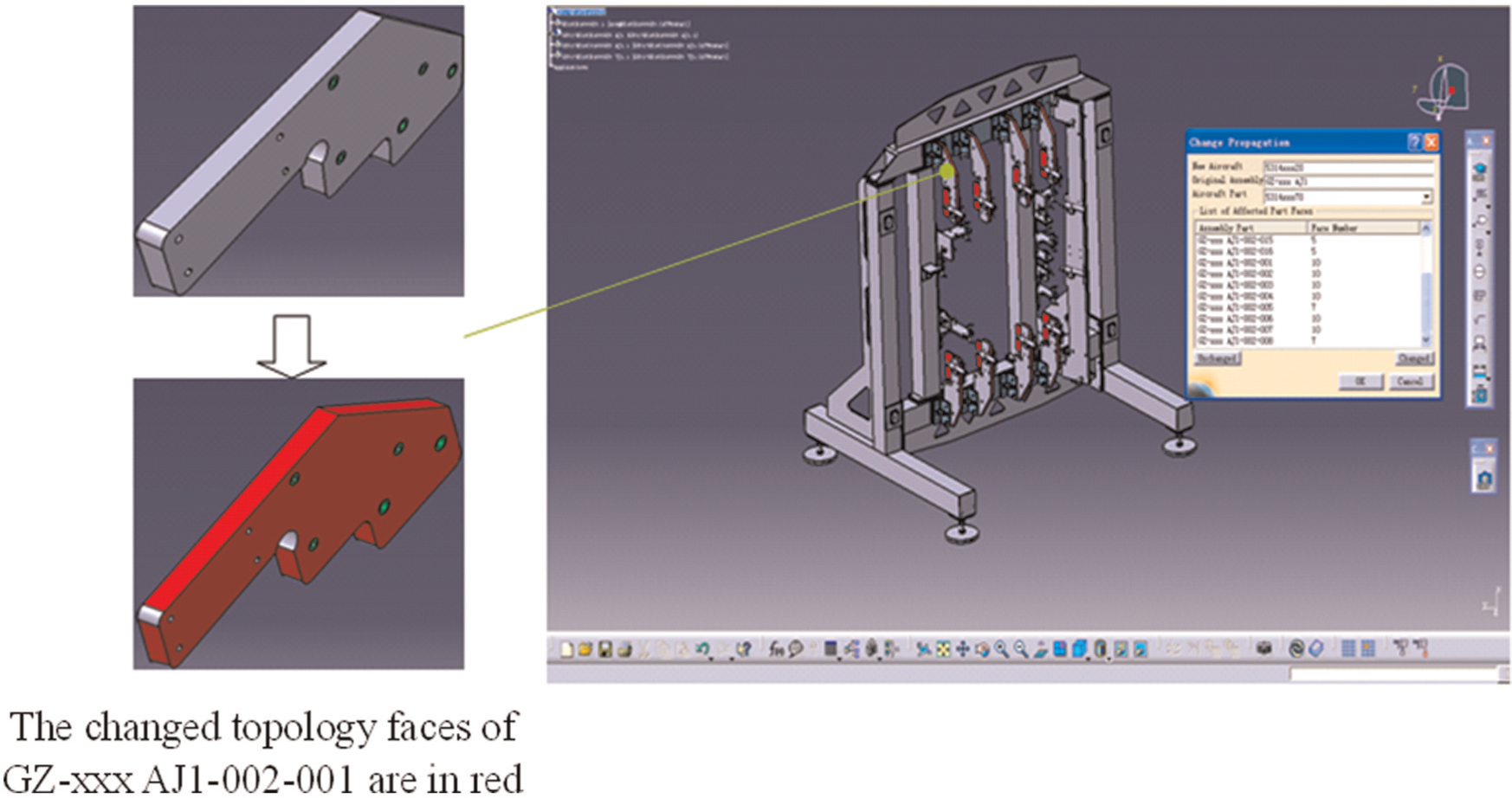
If distances between the short strengthened beams of the aircraft are changed, the change propagation process begins. First, CVs for the short strengthened beams are captured. Then, three types of relation matrices are obtained. After that, changes are propagated to the assembly tooling and the CVs for the influenced assembly tooling parts are computed with the change propagation algorithm. The change propagation process is detailed as follows. First changes are propagated to the topology faces of GZ-xxx AJ1-002-i (i = 009–016) which are marked with red color through the computer-aided system, as shown in Figure 14, due to the constraints between the topology faces of GZ-xxx AJ1-002-i (i = 009–016) and the short strengthened beams. Second changes are propagated to the topology faces of GZ-xxx AJ1-002-i (i = 001–008) which are marked with red color in Figure 15, due to the constraints between the topology faces of GZ-xxx AJ1-002-i (i = 001–008) and GZ-xxx AJ1-002-i (i = 009–016). Then change propagation ends because assembly tooling–assembly tooling RM in the next propagation step is empty. With this computer-aided system, the aircraft designer can conveniently detect the change propagation to the assembly tooling earlier and can further assess the CI qualitatively in a uniform way before the real change implementation.

Figure 14.

First change propagation step.

Figure 15.

Second change propagation step.

Regarding the change propagation results, it is found that 115 topology faces of cardboard subassembly are required to change. Numbers of topology faces required to change are shown in the system window and these topology faces are marked with red color to remind the designers of the potential changes. The number of the topology faces of each part required to change is shown in Table 7. According to these CI indices, predication can be made by designers to assess the CI. For this case, the CI index of GZ-xxx AJ1-002-i (i = 001–008) is relatively lager. The recommendation is that more attention should be paid to the change of GZ-xxx AJ1-002-i (i = 001–008). Besides, in concurrent design of aircraft and assembly tooling, CIs on the assembly tooling vary according to the schemes of aircraft design change. And the minimal influence risk on the assembly tooling is actually expected. Based on the CI index, influence on the assembly tooling can be continuously fed back from the assembly tooling designers to the aircraft designers and recommendations can be provided. In this way, the scheme of aircraft design change with the minimal influence risk on the assembly tooling can be suggested.

Table 7.

CI index of the affected assembly tooling part.

Part name	CI index
GZ-xxx AJ1-002-009	5
GZ-xxx AJ1-002-010	5
GZ-xxx AJ1-002-011	6
GZ-xxx AJ1-002-012	5
GZ-xxx AJ1-002-013	5
GZ-xxx AJ1-002-014	5
GZ-xxx AJ1-002-015	5
GZ-xxx AJ1-002-016	5
GZ-xxx AJ1-002-001	10
GZ-xxx AJ1-002-002	10
GZ-xxx AJ1-002-003	10
GZ-xxx AJ1-002-004	10
GZ-xxx AJ1-002-005	7
GZ-xxx AJ1-002-006	10
GZ-xxx AJ1-002-007	10
GZ-xxx AJ1-002-008	7

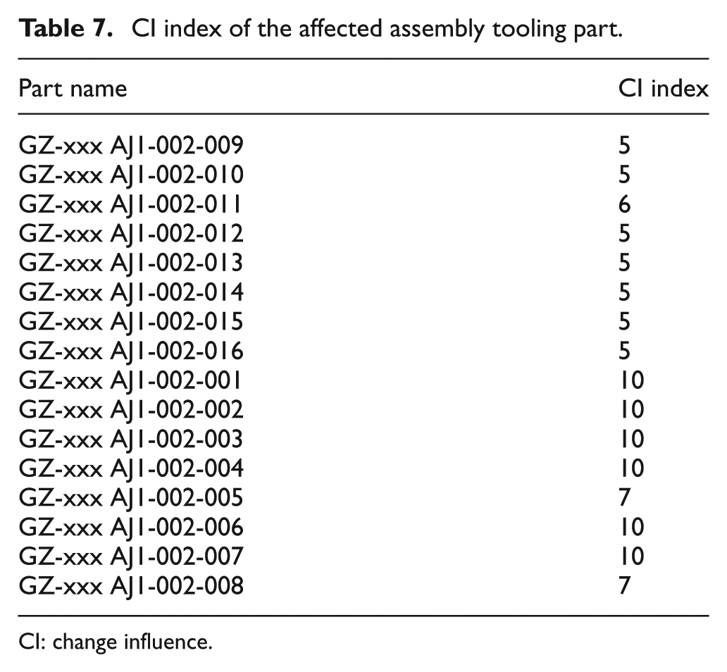
CI: change influence.

Conclusion and future work

In concurrent design, design change in assembly tooling is raised throughout the design change process of aircraft and can cause severe profit losses if not managed efficiently. Using topology faces as basic processing units and focusing on the constraint relation between topology faces, this article provides the rationales for change propagation and allows a more proactive management of changes in assembly tooling design. Four contributions of the article can be highlighted. First, for effective EC management, the shortcomings of DSM constructed at the part or component level were discussed and a practical constraint model at the topology face level was presented. Second, CV representing the changes in topology faces and RM recording change relationships between topology faces were introduced. Third, algorithms to realize the goal of detecting the change propagation from aircraft to assembly tooling were proposed. Fourth, CI index is proposed to assess the influences of changes from aircraft to assembly tooling.

Future work will incorporate the reasoning of relationships between topology faces to construct change relationships more precisely. In addition, this research will also be extended to the change propagation analysis in more aircraft and assembly tooling design cases.