Sage Journals: Discover world-class research

Abstract

This article presents experimental investigation on AISI 1019 steel for study of surface roughness in end milling operation using carbide inserts. The objective of this work is to establish the empirical relationships between the machining parameters and average surface roughness using response surface methodology. The first-order and quadratic models have been developed in terms of feed, cutting speed, depth of cut, and nose radius. Furthermore, the Box–Cox transformation has been employed to improve the prediction ability of the first-order model. The cutting speed, feed, and nose radius seem to have the significant effect on surface roughness.

Keywords

AISI 1019 steel end milling surface roughness response surface methodology Box–Cox transformation

Introduction and literature review

The manufacturing industry is continuously striving to decrease machining costs and improve the surface finish (reduced surface roughness) of the machined parts. Mechanical properties such as fatigue behavior, corrosion resistance, and creep life depend on surface roughness. Thus, surface roughness is an important factor to be taken care of during machining in manufacturing industries. Better surface finish in machining operation can be obtained by proper selection of machining parameters such as cutting speed, feed rate, depth of cut, tool angles, and nose radius. The topic has been quite interesting and useful to research across the spectrum of machining processes.^1–3

Among the various machining parameters, the main parameters affecting the surface roughness are cutting speed, depth of cut, and feed. These three are the primary parameters governing the performance of any basic machining operation. The machine operator has complete control over these parameters. Other factors such as kind of material, type of tool, tool angles, acceleration, and vibrations are also expected to influence the performance, but these are difficult to be controlled by an operator during machining.

In manufacturing industries, the end milling is one of the most commonly used material removal operations for making profiles, slots, pockets, and surface contouring in dies and molds. The widespread usage of end milling operations in manufacturing industries raised a need for developing a systematic approach that can help in achieving the minimum surface roughness, minimum tool wear, minimum cutting forces, and so on. Therefore, the topic has been the focus of the study for several researchers in the past.^4–9

Mansour and Abdalla¹⁰ investigated the effect of cutting speed, feed rate, and axial depth of cut on surface roughness during end milling of EN 32 steel with coated tungsten carbide inserts using response surface methodology (RSM). It has been concluded that surface roughness increases with increase in feed and axial depth of cut, while an increase in the cutting speed decreases the surface roughness.

Ghani et al.⁵ investigated the optimal parametric combination for minimum surface roughness and minimum cutting force in end milling of AISI H13 hardened steel using L₂₇ orthogonal array-based Taguchi approach. The optimal combination of cutting parameters for low resultant cutting force and good surface finish has been obtained at high cutting speed, low feed rate, and small depth of cut.

Wang and Chang¹¹ studied the effect of cutting speed, feed, depth of cut, concavity, and axial relief angles on surface roughness in dry and wet end milling of AL2014-T6 alloy using RSM. The cutting speed, feed, concavity, and axial relief angles have been found significant factors affecting the dry-cut model, while feed and concavity angle were found significant for the wet cutting model.

Reddy and Rao¹² investigated the optimal parametric combination (cutting speed, feed, nose radius, and rake angle) for achieving a better surface finish in dry and wet milling of AISI 1045 steel using RSM. The model obtained has further been optimized by using genetic algorithm (GA). It has been found that proper selection of parameters eliminates the use of cutting fluids during machining and hence makes machining more environmental friendly.

Oktem et al.¹³ investigated the optimal parametric combination to obtain minimum surface roughness during end milling of aluminum 7075-T6 using coated carbide tool. The cutting speed, feed, axial depth of cut, radial depth of cut, and machining tolerance have been considered as machining parameters. The RSM coupled with GA has been used for optimization of machining parameters. It has been observed that the optimum values so obtained correlate very well with the experimentally obtained values.

Chen and Savage¹⁴ developed fuzzy net-based surface roughness prediction model under different tool and workpiece combinations for end milling process. Cutting speed, feed, depth of cut, vibration, tool diameter, tool material, and workpiece material have been considered as input variables for fuzzy system. The result reveals that the developed model displays good capability to predict surface roughness.

Brezocnik et al.¹⁵ studied the influence of cutting conditions (spindle speed, feed rate, depth of cut, and vibrations) on surface roughness in end milling of 6061 aluminum. The authors proposed genetic programming to predict surface roughness values. The result reveals that the surface roughness is most influenced by the feed rate. The developed models have been observed to display good prediction ability.

Iqbal et al.¹⁶ investigated the effects of cutting parameters on tool life and surface roughness in hard milling of AISI D2 steel and X210 Cr12 steel using coated carbide ball-nose end mills. The hardened steel microstructure, workpiece inclination angle, cutting speed, and radial depth of cut have been considered as cutting parameters. The D-optimal base RSM has been employed to develop empirical models for tool life and surface roughness. For the tool life, the workpiece material is found to be the most influential parameter, while for surface roughness the workpiece inclination angle is found to be the most important parameter, the higher the values of inclination angle the better the surface finish.

The review of the research presented above reveals that work has been carried out to investigate the effect of machining parameters on surface roughness obtained during end milling of various ferrous and nonferrous metals. The AISI 1019 steel is widely used as a main engineering material in manufacturing industries, such as automotive, aerospace, and aircraft industries, where superior machinability is the most important factor. A study of surface roughness of the machined part during end milling on this material will be quite useful. The objective of this study is to investigate the effect of cutting parameters (feed, cutting speed, depth of cut, and nose radius) on surface roughness and to develop empirical models to predict the surface roughness during end milling of this material.

Experimental details and measurement

In order to accomplish the objective of this experimental work, end milling experiments were performed on AISI 1019 steel with physical vapor deposition (PVD)-coated carbide inserts on computer numerical control (CNC) machining center. All the machining experiments were carried out in wet conditions. The parameters used in the experiments were feed, cutting speed, depth of cut, and nose radius. The details of experimental setup are given in Table 1.

Table 1.

Details of experimental setup.

Test specimens	AISI 1019 steel plate of size 100 mm × 50 mm × 20 mm
Chemical composition of AISI 1019 steel (wt%)	C 0.19%, Mn 0.5%, Si 0.11%, P 0.027%, S 0.013%
Machine tool	LEADWELL V 40 CNC machining center Continuously variable spindle speed up to 8000 r/min 18.5 kW motor
Cutting inserts	PVD-coated carbide inserts (a) ISO designation of AXMT0903R05 EML (0.5 mm nose radius) (b) ISO designation of AXMT0903R08 EML (0.8 mm nose radius)
End mill	Two-flute end mill having 18 mm diameter with two inserts
Surface roughness tester	Surf coder SE 1200

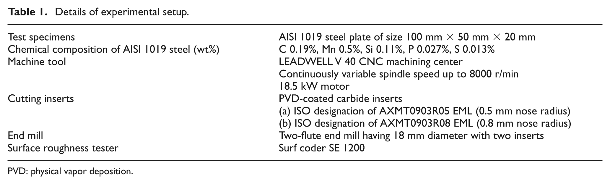
PVD: physical vapor deposition.

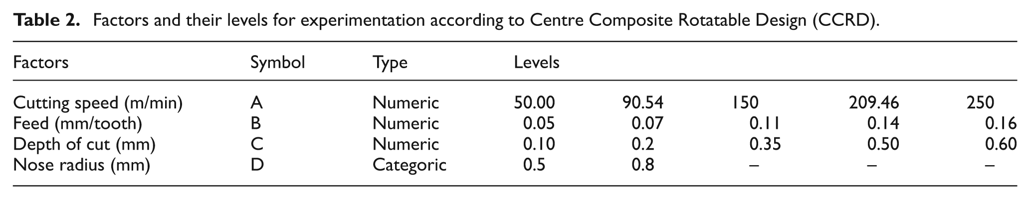
In this study, the experimental design based on RSM has been implemented to analyze the effect of four independent parameters for end milling, that is, cutting speed, feed, depth of cut, and nose radius, on surface roughness. Out of four parameters, feed, cutting speed, and depth of cut are numeric parameters and nose radius is categoric parameter. Table 2 shows machining parameters and their levels.

Table 2.

Factors and their levels for experimentation according to Centre Composite Rotatable Design (CCRD)

Factors	Symbol	Type	Levels
Cutting speed (m/min)	A	Numeric	50.00	90.54	150	209.46	250
Feed (mm/tooth)	B	Numeric	0.05	0.07	0.11	0.14	0.16
Depth of cut (mm)	C	Numeric	0.10	0.2	0.35	0.50	0.60
Nose radius (mm)	D	Categoric	0.5	0.8	–	–	–

Surface roughness is defined as the finer irregularities of the surface texture that usually results from the inherent action of the machining process.¹³ There are many parameters related to surface roughness used in literatures. Among the various roughness parameters, the centerline average (CLA) surface roughness denoted by R_a is the most accepted and widely used parameter in industries.^17–21

A portable surface roughness tester (Surf coder SE 1200) has been used to measure the CLA surface roughness values (R_a) of finish workpieces. It has three measuring modes, namely, skid, skidless, and right angle to drive. In this study, the measurements have been taken in skidless mode according to ISO 97 R standard, which includes Gaussian filter, cutoff length 0.8 mm, and evaluation length 4.0 mm (5 × 0.8 mm).

The measurements have been repeated at three different locations of the finished workpiece in the direction of the tool movement. Finally, the mean of all three CLA surface roughness values (R_a) has been considered for the particular trial.

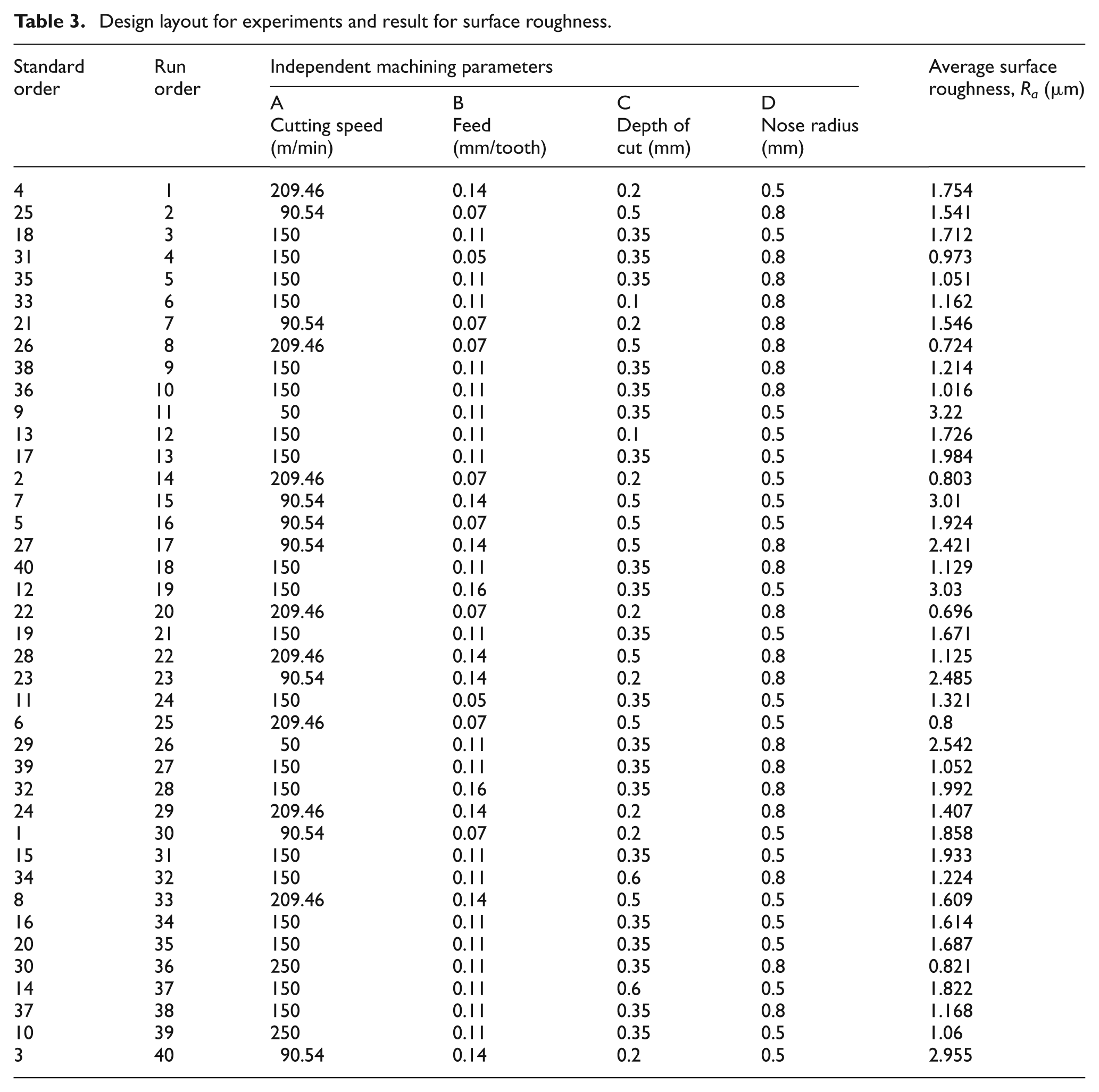
In this research, a total of 40 sets of experiments have been sorted out (20 sets each corresponding to the nose radii 0.5 and 0.8 mm) based on RSM. The complete design layout for experiments and the results obtained as per the experimental plan are shown in Table 3.

Table 3.

Design layout for experiments and result for surface roughness.

Standard order	Run order	Independent machining parameters				Average surface roughness, R_a (µm)
		A	B	C	D
		Cutting speed (m/min)	Feed (mm/tooth)	Depth of cut (mm)	Nose radius (mm)
4	1	209.46	0.14	0.2	0.5	1.754
25	2	90.54	0.07	0.5	0.8	1.541
18	3	150	0.11	0.35	0.5	1.712
31	4	150	0.05	0.35	0.8	0.973
35	5	150	0.11	0.35	0.8	1.051
33	6	150	0.11	0.1	0.8	1.162
21	7	90.54	0.07	0.2	0.8	1.546
26	8	209.46	0.07	0.5	0.8	0.724
38	9	150	0.11	0.35	0.8	1.214
36	10	150	0.11	0.35	0.8	1.016
9	11	50	0.11	0.35	0.5	3.22
13	12	150	0.11	0.1	0.5	1.726
17	13	150	0.11	0.35	0.5	1.984
2	14	209.46	0.07	0.2	0.5	0.803
7	15	90.54	0.14	0.5	0.5	3.01
5	16	90.54	0.07	0.5	0.5	1.924
27	17	90.54	0.14	0.5	0.8	2.421
40	18	150	0.11	0.35	0.8	1.129
12	19	150	0.16	0.35	0.5	3.03
22	20	209.46	0.07	0.2	0.8	0.696
19	21	150	0.11	0.35	0.5	1.671
28	22	209.46	0.14	0.5	0.8	1.125
23	23	90.54	0.14	0.2	0.8	2.485
11	24	150	0.05	0.35	0.5	1.321
6	25	209.46	0.07	0.5	0.5	0.8
29	26	50	0.11	0.35	0.8	2.542
39	27	150	0.11	0.35	0.8	1.052
32	28	150	0.16	0.35	0.8	1.992
24	29	209.46	0.14	0.2	0.8	1.407
1	30	90.54	0.07	0.2	0.5	1.858
15	31	150	0.11	0.35	0.5	1.933
34	32	150	0.11	0.6	0.8	1.224
8	33	209.46	0.14	0.5	0.5	1.609
16	34	150	0.11	0.35	0.5	1.614
20	35	150	0.11	0.35	0.5	1.687
30	36	250	0.11	0.35	0.8	0.821
14	37	150	0.11	0.6	0.5	1.822
37	38	150	0.11	0.35	0.8	1.168
10	39	250	0.11	0.35	0.5	1.06
3	40	90.54	0.14	0.2	0.5	2.955

Analysis of variance

The outcome of experiments performed as per the experimental plan is shown in Table 3 along with the run order selected at random. Further analysis of these data was carried out using the Design Expert 8.0.4.1 software.

Analysis of variance for first-order model

Analysis of variance (ANOVA) is commonly used to perform test for (1) significance of the regression model, (2) significance on individual model coefficients, and (3) lack of fit of model. This analysis is based on two assumptions: (1) the variables are normally distributed and (2) homogeneity of variance. Significant violation of either assumption can increase the chances of committing either a Type I or II error depending on the nature of the analysis and violation of the assumption. The normal probability plot of the residuals is shown in Figure 1 to examine the viability of assumptions of ANOVA for residuals.

Figure 1.

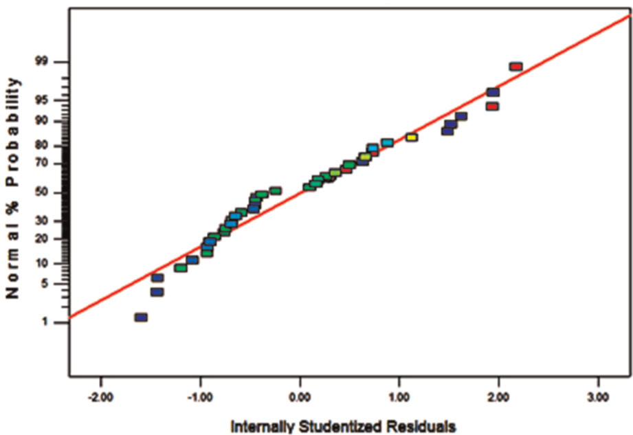
Normal probability plot of the residuals (first-order model).

The normal probability plot indicates the behavior of residuals whether the residuals follow a normal distribution or not. If the residuals follow a normal distribution, maximum number of points should fall on the straight line. Figure 1 reveals that some of the residuals are lying outside the straight line, thus not completely following the normal distribution.

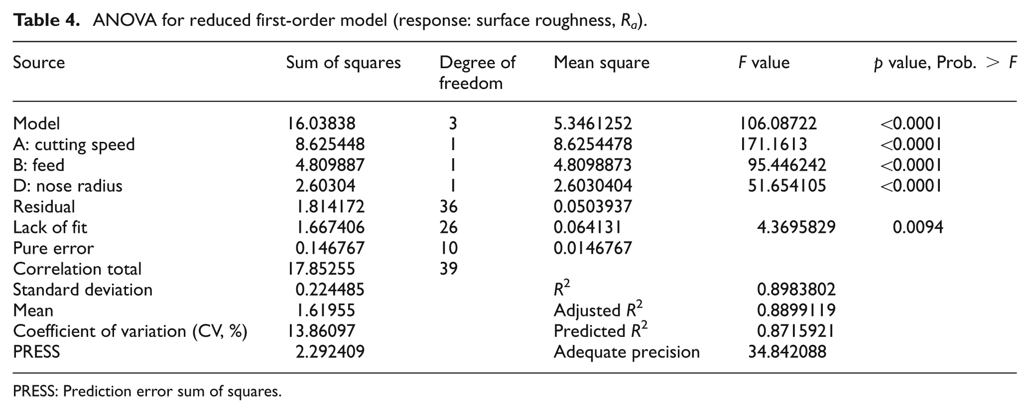
Table 4 represents the ANOVA for the reduced first-order model for surface roughness by selecting the backward elimination procedure to eliminate insignificant terms. This analysis has been carried out for a significance level of α = 0.05, that is, for a confidence interval of 95%. The table shows that the value of “Prob. > F” for model is 0.0001, which is less than 0.05, which indicates that the model is significant, that is, the terms in the model have a significant effect on the response. In the same manner, the values of “Prob. > F” for cutting speed, feed, and nose radius are less than 0.05, indicating that these terms are significant.

Table 4.

ANOVA for reduced first-order model (response: surface roughness, R_a)

Source	Sum of squares	Degree of freedom	Mean square	F value	p value, Prob. > F
Model	16.03838	3	5.3461252	106.08722	<0.0001
A: cutting speed	8.625448	1	8.6254478	171.1613	<0.0001
B: feed	4.809887	1	4.8098873	95.446242	<0.0001
D: nose radius	2.60304	1	2.6030404	51.654105	<0.0001
Residual	1.814172	36	0.0503937
Lack of fit	1.667406	26	0.064131	4.3695829	0.0094
Pure error	0.146767	10	0.0146767
Correlation total	17.85255	39
Standard deviation	0.224485		R ²	0.8983802
Mean	1.61955		Adjusted R²	0.8899119
Coefficient of variation (CV, %)	13.86097		Predicted R²	0.8715921
PRESS	2.292409		Adequate precision	34.842088

PRESS: Prediction error sum of squares.

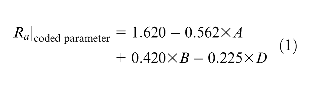
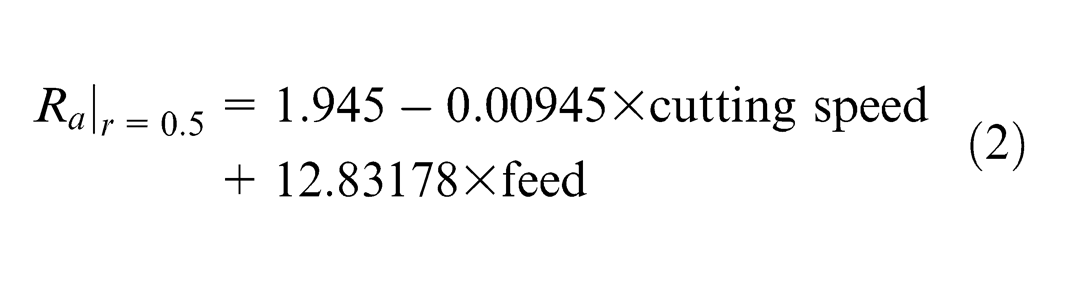
The R² value, which is the measure of proportion of total variability explained by the model, is equal to 0.8983. The adjusted R² value is equal to 0.8899; it is particularly useful when comparing models with different number of terms. The result shows that the adjusted R² value is very close to the ordinary R² value. The final empirical model for surface roughness in terms of coded factors is represented in equation (1). The final empirical models in terms of actual factors are given in equations (2) and (3) for nose radii 0.5 and 0.8 mm, respectively

\begin{matrix} {R_{a} |}_{coded parameter} & = 1.620 - 0.562 \times A \\ + 0.420 \times B - 0.225 \times D \end{matrix}

(1)

\begin{matrix} {R_{a} |}_{r = 0.5} & = 1.945 - 0.00945 \times cutting speed \\ + 12.83178 \times feed \end{matrix}

(2)

\begin{matrix} {R_{a} |}_{r = 0.8} & = 1.434 - 0.00945 \times cutting speed \\ + 12.83178 \times feed \end{matrix}

(3)

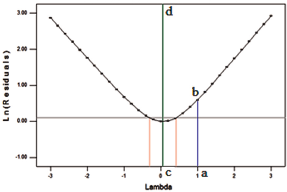
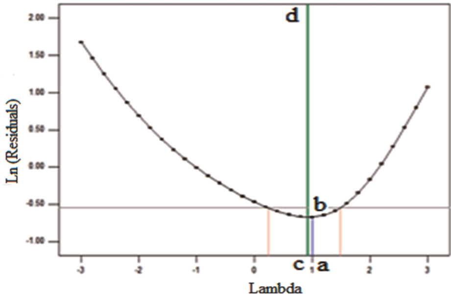
The results obtained from the first-order model have been improved using the Box–Cox transformation. This approach provides a family of transformations to normalize the data by identifying an appropriate exponent “Lambda or λ.” The “Lambda” value indicates the power to which all the data are raised to obtain the normalized set of data. Box and Cox originally envisioned this transformation as a panacea for simultaneously correcting normality, linearity, and homogeneity.²²

Figure 2 shows Box–Cox plot for power transformation of residuals. The line “a–b” indicates the current value of Lambda for residuals ( $λ_{a - b} = 1$ ), lying outside the 95% confidence limits. But the best recommended value of Lambda is approximately 0.05 as shown by line “c–d.” Thus, according to Box–Cox transformation, the natural log transformation on the response makes the residuals normally distributed.²²

Figure 2.

Box–Cox plot for power transformation (first-order model).

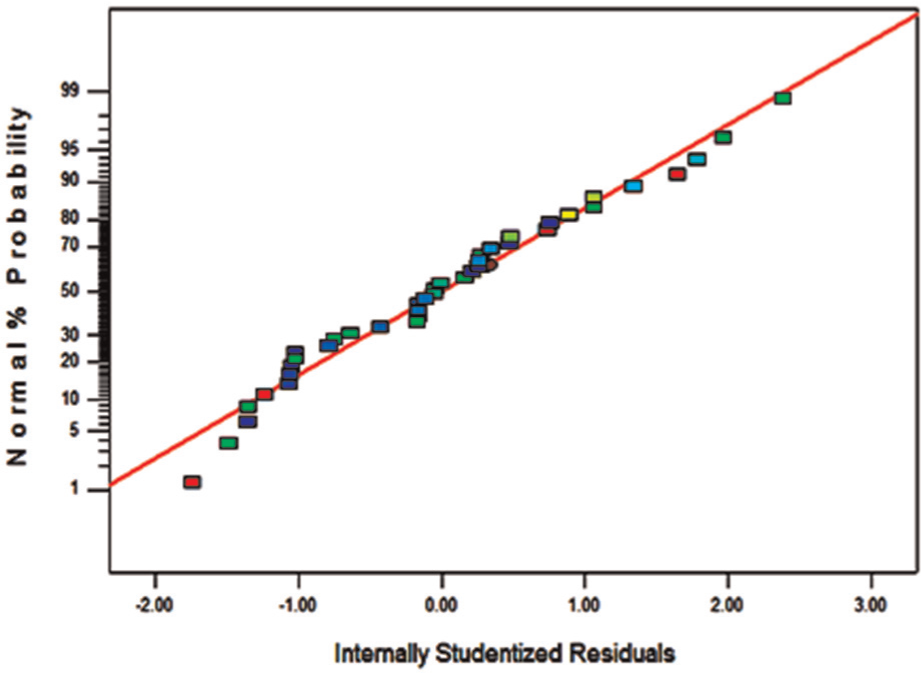
Figure 3 shows the normal distribution plot for residuals after the Box–Cox transformation. This figure shows that the most of the residuals fall on the straight line indicating that the residuals are distributed normally.

Figure 3.

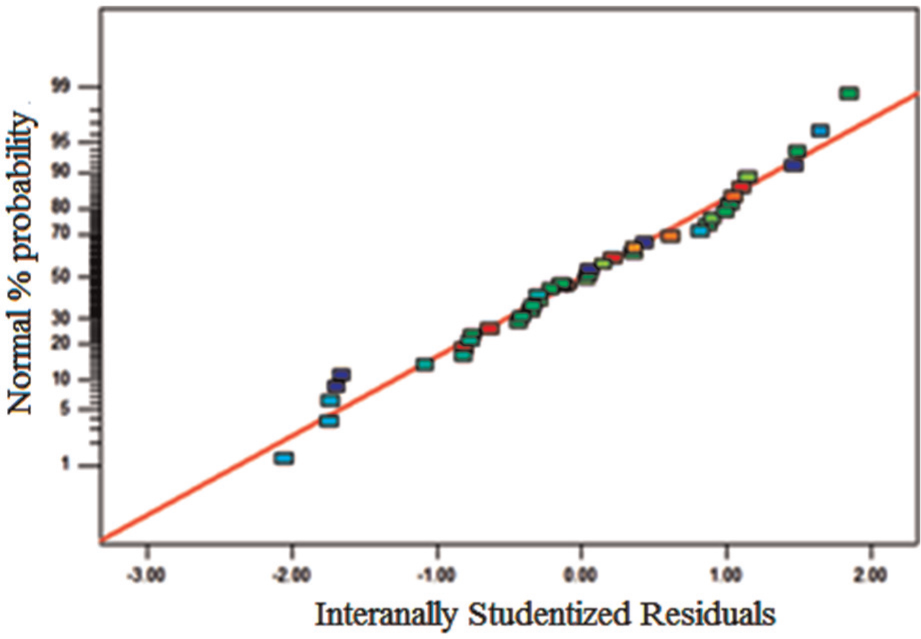
Normal probability plot for residuals after the Box–Cox transformation (first-order model).

Table 5 represents the ANOVA for the reduced first-order model for surface roughness after Box–Cox transformation. It is clear from Table 5 that the model is still significant. The terms cutting speed, feed, and nose radius are also the significant model terms. The value of “Prob. > F” for lack of fit is 0.0680, which is greater than 0.05. This indicates that lack of fit is insignificant. This is desirable to fit a model.

Table 5.

ANOVA for reduced first-order model after transformation (response: surface roughness, R_a).

Source	Sum of squares	Degree of freedom	Mean square	F value	p value, Prob. > F
Model	6.1830	3	2.0610	165.997	<0.0001
A: cutting speed	3.3198	1	3.3198	267.386	<0.0001
B: feed	1.8268	1	1.8268	147.134	<0.0001
D: nose radius	1.0364	1	1.0364	83.472	<0.0001
Residual	0.4470	36	0.0124
Lack of fit	0.3867	26	0.0149	2.470	0.0680
Pure error	0.0602	10	0.0060
Correlation total	6.6300	39
Standard deviation	0.111427		R ²		0.9326
Mean	0.399616		Adjusted R²		0.927
Coefficient of variation (CV, %)	27.88343		Predicted R²		0.9163
PRESS	0.554862		Adequate precision		43.604

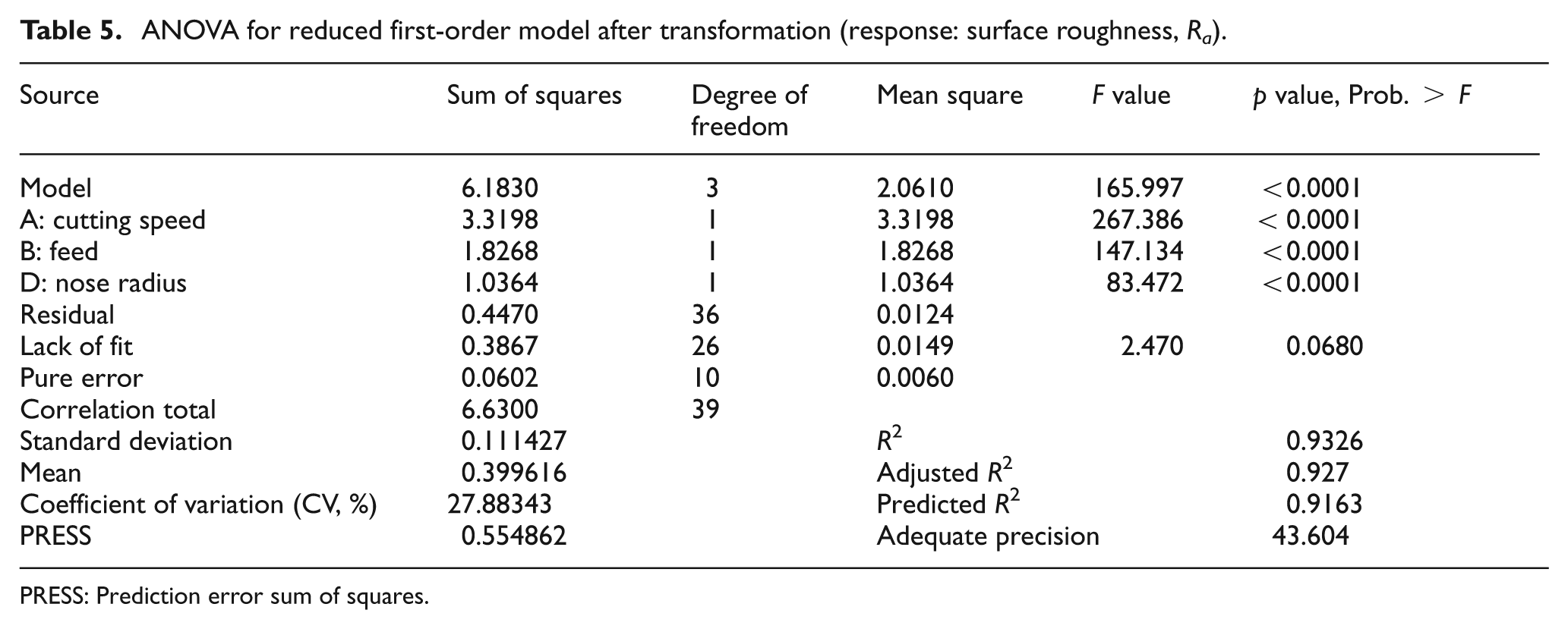
PRESS: Prediction error sum of squares.

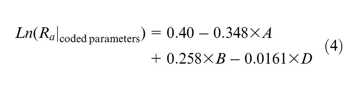
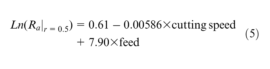
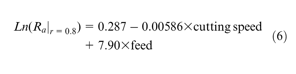
The R² value and adjusted R² value are 0.9326 and 0.927, respectively. The final regression model after transformation for surface roughness in terms of coded factors is represented in equation (4), and final empirical models in terms of actual factors are given in equations (5) and (6) for nose radii 0.5 and 0.8 mm, respectively

\begin{matrix} Ln ({R_{a} |}_{coded parameters}) & = 0.40 - 0.348 \times A \\ + 0.258 \times B - 0.0161 \times D \end{matrix}

(4)

\begin{matrix} Ln {(R_{a} |}_{r = 0.5}) & = 0.61 - 0.00586 \times cutting speed \\ + 7.90 \times feed \end{matrix}

(5)

\begin{matrix} Ln ({R_{a} |}_{r = 0.8}) & = 0.287 - 0.00586 \times cutting speed \\ + 7.90 \times feed \end{matrix}

(6)

ANOVA for quadratic model

Figure 4 shows Box–Cox power transformation plot for quadratic model. In this figure, line “a–b” indicates $λ_{a - b} = 1$ , at 95% confidence interval, and the best recommended value $λ_{c - d} ≅ 0.93$ is shown by line “c–d.” As the current value is very close to the best recommended value of Lambda, no transformation is desirable. The normal probability plot of the residuals for quadratic model is shown in Figure 5.

Figure 4.

Box–Cox power transformation plot (quadratic model).

Figure 5.

Normal probability plot of residuals for R_a data (quadratic model).

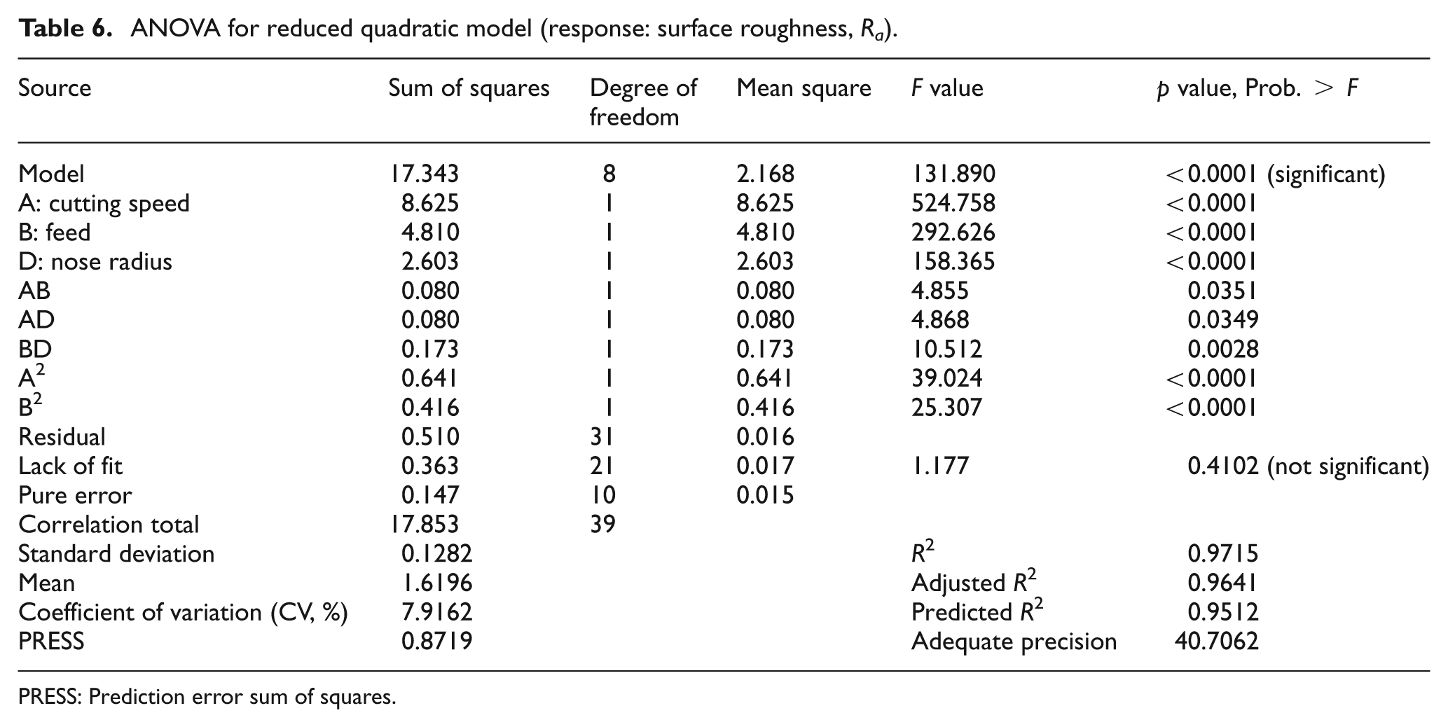
The ANOVA for response surface reduced quadratic model for surface roughness by selecting the backward elimination procedure is summarized in Table 6. This table shows that the value of “Prob. > F” for model is 0.0001 (i.e. <0.05), which indicates that the model is significant, that is, the terms in the model have a significant effect on the response. In the same manner, the value of “Prob. > F” for main effect of cutting speed, feed, and nose radius; two-level interaction of cutting speed and feed, cutting speed and nose radius, and feed and nose radius; and second-order effect of cutting speed and feed are less than 0.05, indicating that these are the significant model terms. The value of “Prob. > F” for lack of fit is 0.4102 (i.e. >0.05), which indicates that the lack of fit is insignificant.

Table 6.

ANOVA for reduced quadratic model (response: surface roughness, R_a).

Source	Sum of squares	Degree of freedom	Mean square	F value	p value, Prob. > F
Model	17.343	8	2.168	131.890	<0.0001 (significant)
A: cutting speed	8.625	1	8.625	524.758	<0.0001
B: feed	4.810	1	4.810	292.626	<0.0001
D: nose radius	2.603	1	2.603	158.365	<0.0001
AB	0.080	1	0.080	4.855	0.0351
AD	0.080	1	0.080	4.868	0.0349
BD	0.173	1	0.173	10.512	0.0028
A²	0.641	1	0.641	39.024	<0.0001
B²	0.416	1	0.416	25.307	<0.0001
Residual	0.510	31	0.016
Lack of fit	0.363	21	0.017	1.177	0.4102 (not significant)
Pure error	0.147	10	0.015
Correlation total	17.853	39
Standard deviation	0.1282			R ²	0.9715
Mean	1.6196			Adjusted R²	0.9641
Coefficient of variation (CV, %)	7.9162			Predicted R²	0.9512
PRESS	0.8719			Adequate precision	40.7062

PRESS: Prediction error sum of squares.

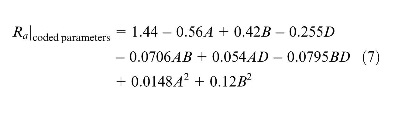
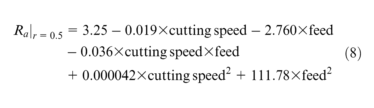
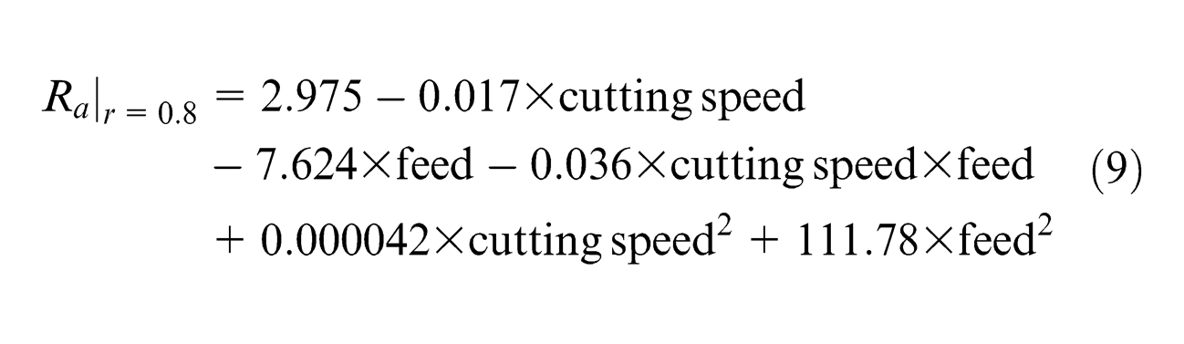
The R² value and adjusted R² value are equal to 0.9715 and 0.9641, respectively. The adequate precision value is equal to 40.7062, which is a ratio of signal to noise. A ratio greater than 4 is desirable, which indicates adequate model discrimination. The adequate precision value compares the range of the predicted values at the design points to the average prediction error. The final regression model for surface roughness in terms of coded factors is represented in equation (7). The final empirical models in terms of actual factors are given in equations (8) and (9) for nose radii 0.5 and 0.8 mm, respectively

\begin{matrix} {R_{a} |}_{coded parameters} & = 1.44 - 0.56 A + 0.42 B - 0.255 D \\ - 0.0706 AB + 0.054 AD - 0.0795 BD \\ + 0.0148 A^{2} + 0.12 B^{2} \end{matrix}

(7)

\begin{matrix} {R_{a} |}_{r = 0.5} & = 3.25 - 0.019 \times cutting speed - 2.760 \times feed \\ - 0.036 \times cutting speed \times feed \\ + 0.000042 \times cutting spee d^{2} + 111.78 \times fee d^{2} \end{matrix}

(8)

\begin{matrix} {R_{a} |}_{r = 0.8} & = 2.975 - 0.017 \times cutting speed \\ - 7.624 \times feed - 0.036 \times cutting speed \times feed \\ + 0.000042 \times cutting spee d^{2} + 111.78 \times fee d^{2} \end{matrix}

(9)

Results and discussion

Influence of machining parameters on surface roughness

In order to investigate the effects of the machining parameters (feed, cutting speed, depth of cut, and nose radius) on surface roughness, the plots between machining parameters and surface roughness have been generated using quadratic model prediction values.

Influence of nose radius on the average surface roughness at constant feed 0.11 mm/tooth, constant depth of cut 0.35 mm, and constant cutting speed 150 m/min is shown in Figure 6. Other machining parameters remaining constant, the surface roughness decreases with increase in nose radius.

Figure 6.

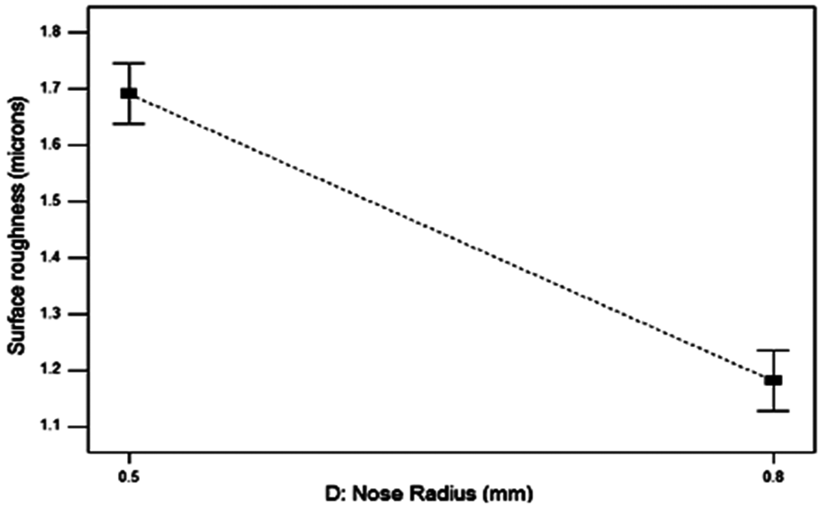
Plot between nose radius and surface roughness.

Figure 7 shows interaction plot between nose radius and speed, when other parameters are kept constant. From this interaction plot, the following facts are revealed: (1) The surface roughness decreases with increase in cutting speed. The rate of variation (decrease) in surface roughness also continuously decreases with increase in cutting speed. (2) Larger nose radius corresponds to smaller value of surface roughness for the range of cutting speed. (3) The effect of nose radius on the surface roughness is also visible from the vertical gap between the two curves corresponding to the two values of nose radius, and the maximum effect appears at minimum cutting speed.

Figure 7.

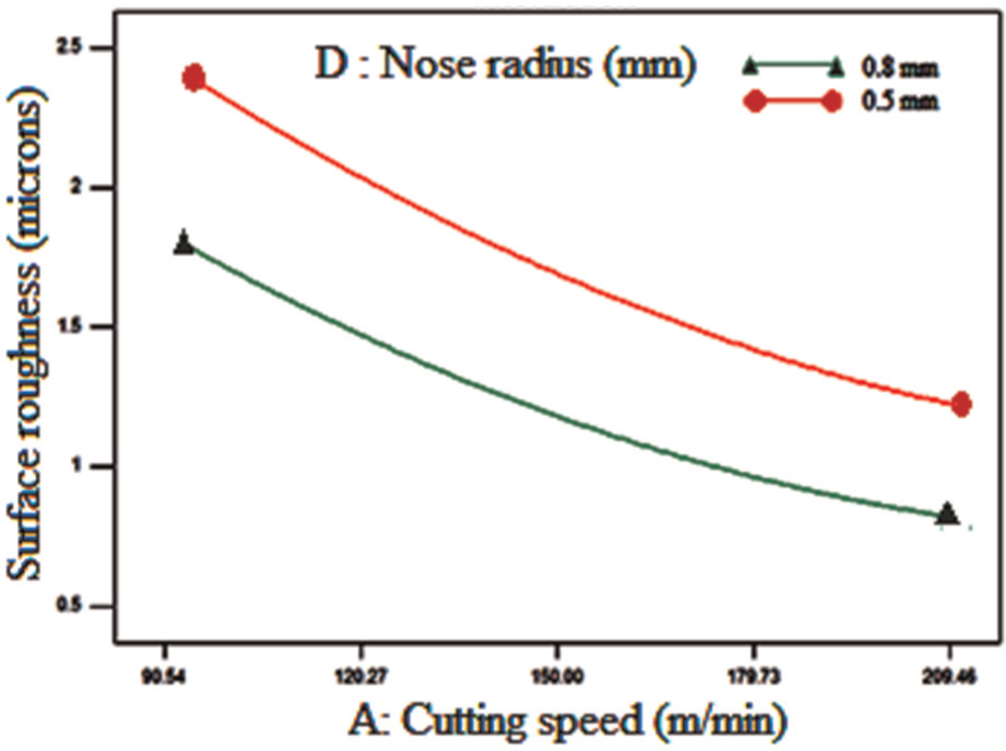
Interaction plot between nose radius and cutting speed at feed 0.11 mm/tooth and depth of cut 0.35 mm for R_a.

Interaction plot between nose radius and feed, keeping other parameters constant, is shown in Figure 8. From this interaction plot, the following facts have been revealed: (1) The surface roughness increases with increase in feed. The rate of variation (increase) in surface roughness also continuously increases with increase in feed. (2) Larger nose radius corresponds to smaller value of surface roughness for the range of feed. (3) The effect of nose radius on the surface roughness is also visible from the vertical gap between the two curves corresponding to the two values of nose radius. The maximum effect caused by variation in nose radius appears at maximum feed.

Figure 8.

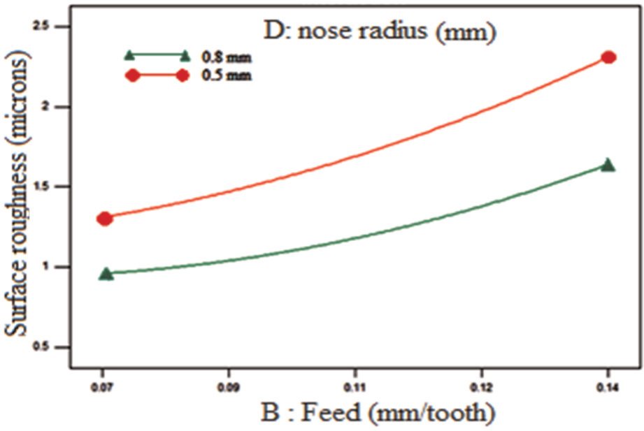
Interaction plot between nose radius and feed at cutting speed 150 m/min and depth of cut 0.35 mm for R_a.

The three-dimensional (3D) surface plots for surface roughness for nose radii 0.5 and 0.8 mm at constant depth of cut 0.35 mm are shown in Figures 9 and 10, respectively. From both the plots, it is explicable that as the cutting speed increases the surface roughness decreases, on the contrary as feed increases surface roughness also increases. This is due to the fact that at higher feed rate, tool traverses the workpiece too fast, resulting in deteriorated surface quality, while higher cutting speed increases the temperature during cutting, which softens the material to enhance the cutting performance leading to reduced surface roughness. These plots reveal that the minimum surface roughness is obtained at low level of feed, high level of speed, and high level of nose radius.

Figure 9.

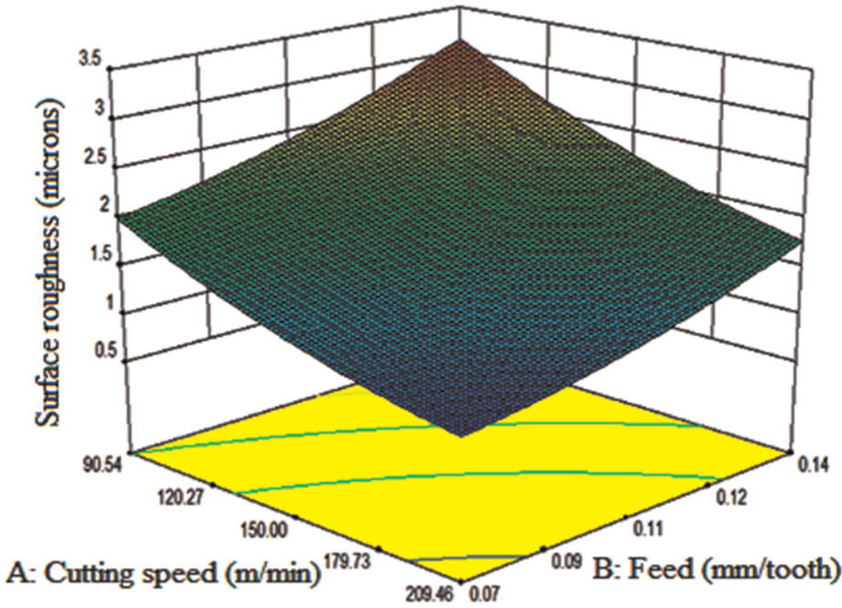
3D surface graph for surface roughness at depth of cut 0.35 mm and nose radius 0.5 mm.

Figure 10.

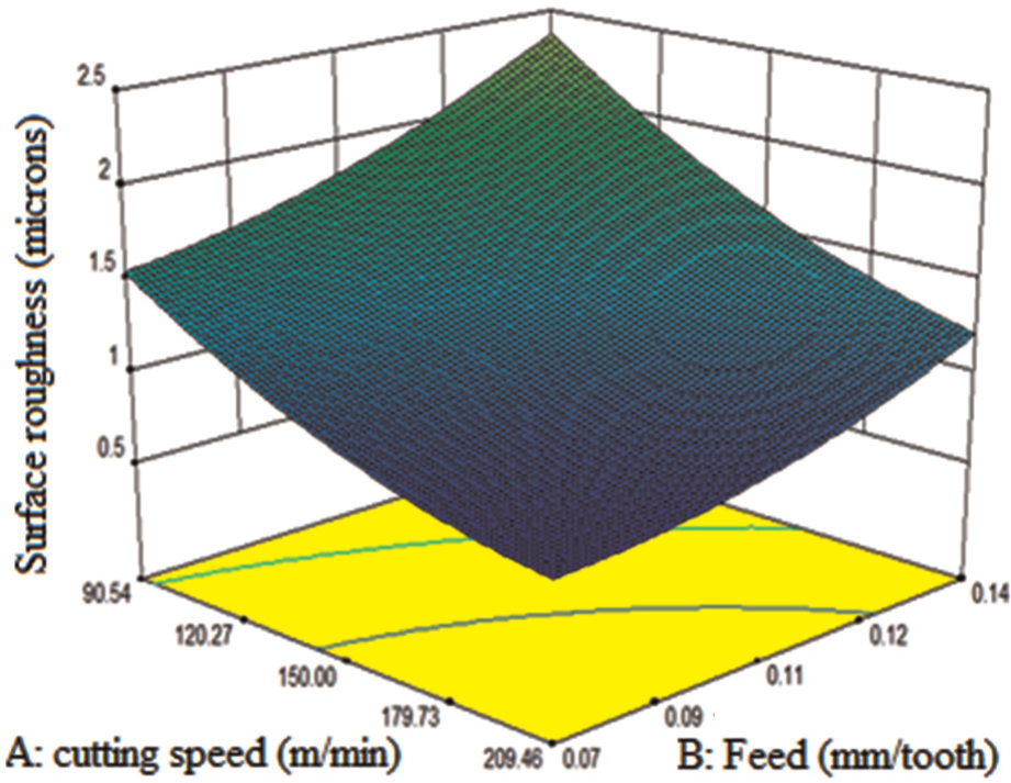
3D surface graph for surface roughness at depth of cut 0.35 mm and nose radius 0.8 mm.

Figure 11 represents the cube plot that shows the three-factor interaction, among feed, cutting speed, and nose radius. According to the plot, the surface roughness is significantly minimized (R_a = 0.672133 µm) when the feed is set to the low level (0.07 mm/tooth), speed at high level (209.67 m/min), and the nose radius at high level (0.8 mm).

Figure 11.

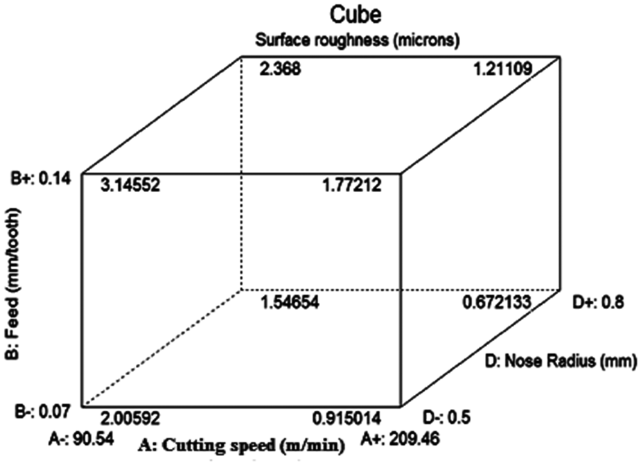
Cube plot for surface roughness at depth of cut 0.35 mm.

The percentage contribution of the significant terms on surface roughness in quadratic model is shown in Figure 12. This figure shows that the cutting speed is the dominant factor affecting the surface roughness among all machining parameters with 49.76% contribution, followed by the feed with contribution of 27.8% and the nose radius with contribution of 15%.

Figure 12.

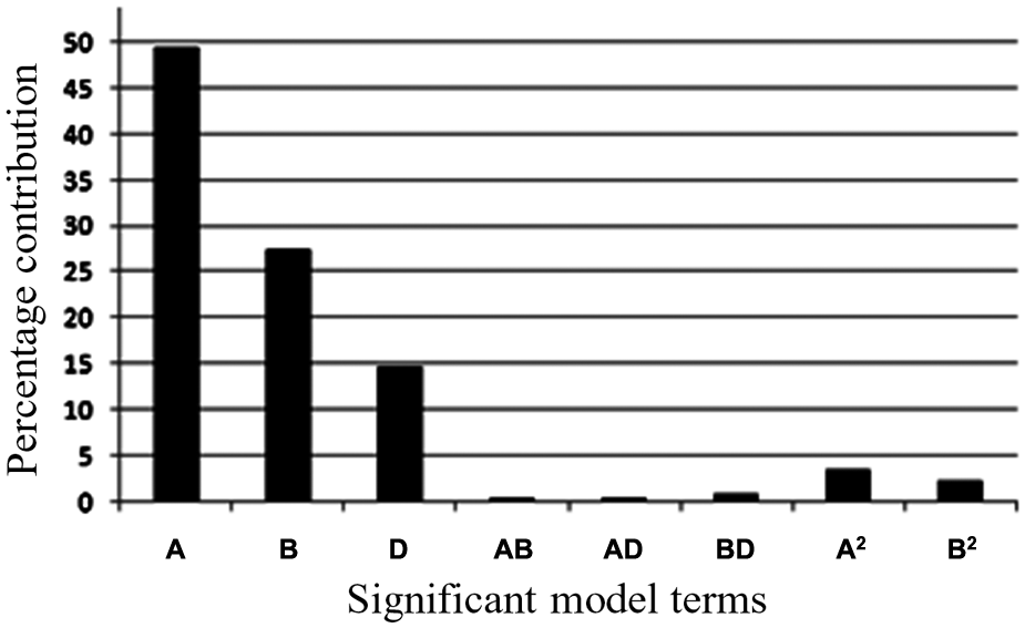
Bar chart for percentage contribution.

Error analysis for prediction models

In order to know the prediction ability of models, a comparison has been made on the basis of the statistical methods of percentage mean absolute error, percentage mean square error, and correlation coefficient (R² values). These values are determined using equations (10) and (11). Table 7 represents the comparative assessment of the results obtained using the first-order prediction models and the quadratic model for the entire data set

% Mean absolute error = (\frac{1}{n} \sum_{i} | \frac{e_{i} - p_{i}}{e_{i}} |) \times 100

(10)

% Mean square error (MSE) = (\frac{1}{n} \sum_{i} {| e_{i} - p_{i} |}^{2}) \times 100

(11)

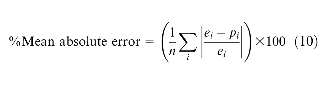
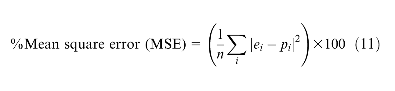
where e is the experimental value, p is the predicted value, and n is the number of treatments for experimentation.

Table 7.

Comparison of predicted surface roughness with experimental values.

Run order	Surface roughness, R_a (µm)
	Experimental	Predicted
		First-order model without transformation	First-order model with transformation	Quadratic model
1	1.858	2.017	1.917	2.006
2	0.803	0.893	0.954	0.915
3	2.955	2.856	3.215	3.146
4	1.754	1.732	1.601	1.772
5	1.924	2.017	1.917	2.006
6	0.8	0.893	0.954	0.915
7	3.01	2.856	3.215	3.146
8	1.609	1.732	1.601	1.772
9	3.22	2.820	3.148	3.148
10	1.06	0.930	0.975	1.075
11	1.321	1.169	1.134	1.190
12	3.03	2.580	2.706	2.869
13	1.726	1.875	1.752	1.692
14	1.822	1.875	1.752	1.692
15	1.933	1.875	1.752	1.692
16	1.614	1.875	1.752	1.692
17	1.984	1.875	1.752	1.692
18	1.712	1.875	1.752	1.692
19	1.671	1.875	1.752	1.692
20	1.687	1.875	1.752	1.692
21	1.546	1.507	1.389	1.547
22	0.696	0.383	0.692	0.672
23	2.485	2.346	2.330	2.368
24	1.407	1.222	1.160	1.211
25	1.541	1.507	1.389	1.547
26	0.724	0.383	0.692	0.672
27	2.421	2.346	2.330	2.368
28	1.125	1.222	1.160	1.211
29	2.542	2.310	2.282	2.455
30	0.821	0.419	0.706	0.747
31	0.973	0.659	0.822	0.948
32	1.992	2.070	1.961	2.092
33	1.162	1.364	1.270	1.181
34	1.224	1.364	1.270	1.181
35	1.051	1.364	1.270	1.181
36	1.016	1.364	1.270	1.181
37	1.168	1.364	1.270	1.181
38	1.214	1.364	1.270	1.181
39	1.052	1.364	1.270	1.181
40	1.129	1.364	1.270	1.181

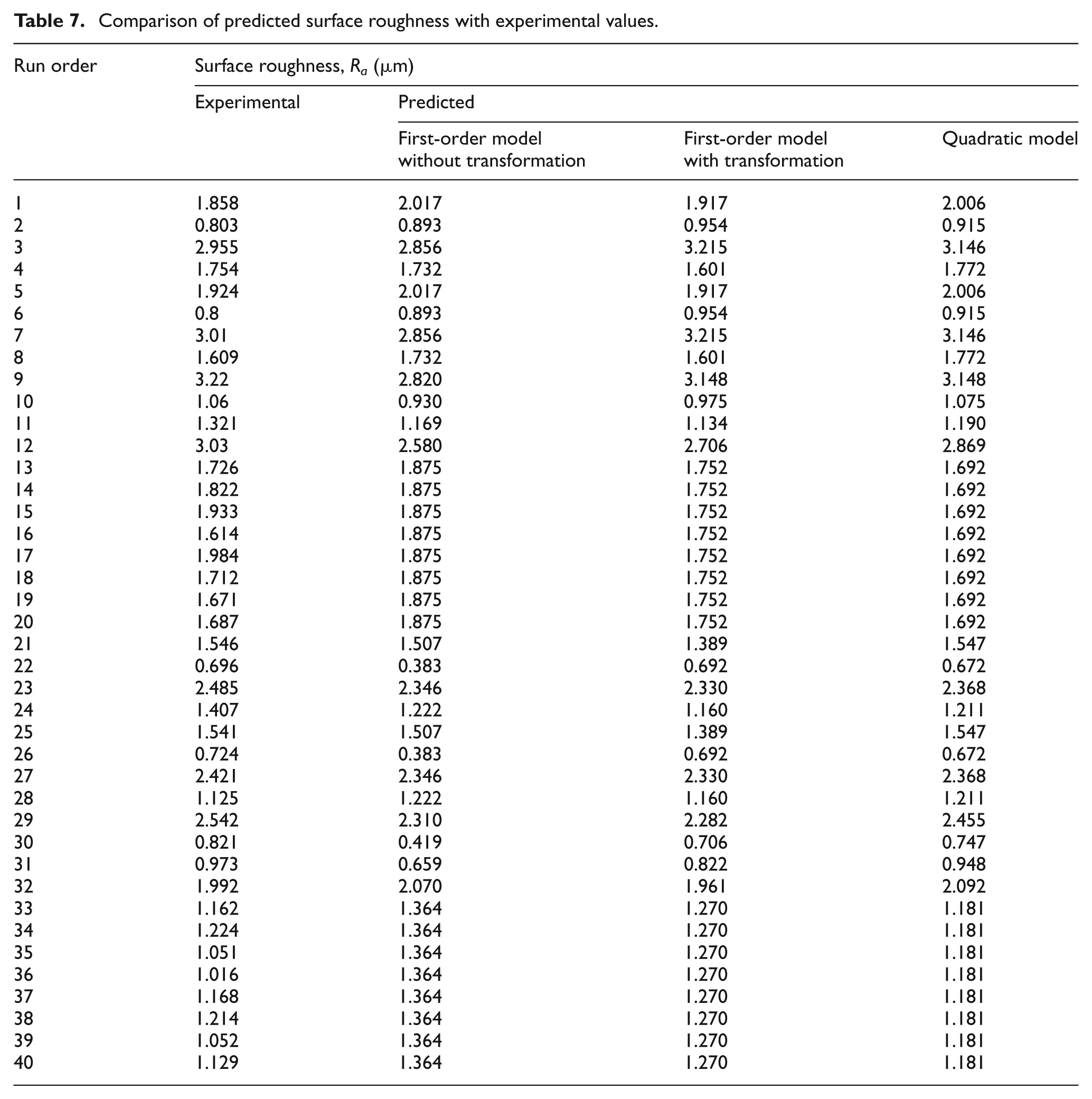
Figure 13 shows the comparison between the absolute errors calculated on the basis of results obtained using first-order models and quadratic model. This figure shows that the percentage absolute errors calculated using the first-order model without transformation are much higher than the absolute errors calculated on the basis of the first-order model with transformation and the quadratic model.

Figure 13.

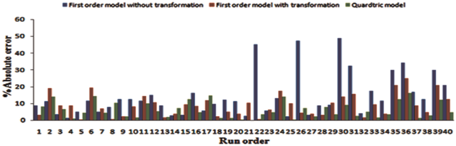
Comparison of absolute errors corresponding to (a) first-order model without transformation, (b) first-order model with transformation, and (c) quadratic model.

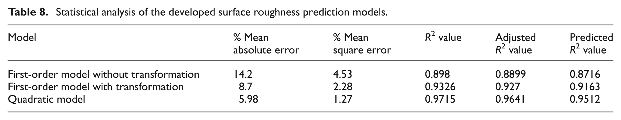
Table 8 represents the comparative assessment of the results obtained using the first-order models and the quadratic model for the entire data set on the basis of percentage absolute error, percentage mean square error, R² value, adjusted R² value, and predicted R² value. It is clearly observed that a significant difference persists between the statistical errors and R² values obtained from the first-order models and the quadratic models.

Table 8.

Statistical analysis of the developed surface roughness prediction models.

Model	% Mean absolute error	% Mean square error	R ² value	Adjusted R² value	Predicted R² value
First-order model without transformation	14.2	4.53	0.898	0.8899	0.8716
First-order model with transformation	8.7	2.28	0.9326	0.927	0.9163
Quadratic model	5.98	1.27	0.9715	0.9641	0.9512

Conclusion and future scope

This article presents an investigation into the effect of machining parameters on surface roughness during end milling of AISI 1019 steel. An attempt has been made to obtain empirical relationship between the cutting parameters and surface roughness in the form of first-order and quadratic models. Among all the empirically developed relationships, quadratic model has been found to indicate better prediction capability.

The following conclusions are derived from this study:

The cutting speed, feed, and nose radius have been found to be the significant parameters, while the depth of cut has shown negligible influence on surface roughness in all the empirically developed relationships. The results clearly illustrate that surface roughness increases with increase in the feed rate, while an increase in the cutting speed and nose radius decreases the surface roughness. Also, the effect of nose radius on the surface roughness has the maximum effect at minimum cutting speed and maximum feed.

The quadratic model indicates the highest contribution of cutting speed on surface roughness (49.76%), followed by the feed (27.8%) and nose radius (15%).

The minimum surface roughness (R_a = 0.672 µm) is achieved at low level of feed (0.07 mm/tooth), at high level of cutting speed (209.67 m/min), and at high level of nose radius (0.8 mm).

The statistical analysis of first-order models indicates that the Box–Cox transformation has a strong potential to improve the prediction ability. In this study, this has reduced the statistical errors, that is, mean absolute error (14.2%–8.7%) and mean square error (4.53%–2.28%).

As the experimental study is based on only two values of nose radii, it may not be appropriate to statistically generalize the result. However, the observation of the effect of the nose radii on surface roughness is important and an indicative one.

In this study, the machining parameters considered are cutting speed, feed, depth of cut, and nose radius. Other factors such as workpiece material, tool material, tool geometry (tool angles, more values of nose radius, and so on), acceleration, and vibrations may also influence the machining performance. An exhaustive study considering all these parameters shall be more useful.

In this study, the CLA value (denoted by R_a) has been adopted as the measure for the surface roughness. A better approach would be to consider other measures for the roughness, such as R_q (also denoted by R_RMS; i.e. root mean square value) and R_z (i.e. maximum peak to valley as well).

Footnotes

Acknowledgements

The cooperation extended by Premium Mold, Chandigarh, for facilitating the conduct of machining experiments has been quite encouraging. The efforts made by anonymous referees in going through this article and making useful comments are gratefully acknowledged.

Declaration of conflicting interests

The authors declare that there is no conflict of interest.

Funding

This research received no specific grant from any funding agency in the public, commercial, or not-for-profit sectors.

References

Davin

. A note on the determination of optimal cutting conditions for surface finish obtained in turning using design of experiments. J Mater Process Tech 2001; 116: 305–308.

Kopac

Bahor

Sokovic

. Optimal machining parameters for achieving the desired surface roughness in fine turning of cold pre-formed steel workpieces. Int J Mach Tool Manu 2002; 42: 707–716.

Ndaliman

Khan

Ali

. Influence of electrical discharge machining process parameters on surface micro-hardness of titanium alloy. Proc IMechE, Part B: J Engineering Manufacture 2013; 227: 460–464.

Alauddin

El Baradie

Hashmi

MSJ

. Computer-aided analysis of a surface-roughness model for end milling. J Mater Process Tech 1995; 55: 123–127.

Ghani

Choudhury

Hassan

. Application of Taguchi method in the optimization of end milling parameters. J Mater Process Tech 2003; 145: 84–92.

. An adaptive-network based fuzzy inference system for prediction of workpiece surface roughness in end milling. J Mater Process Tech 2003; 142: 665–675.

Reddy

Rao

. Experimental investigation to study the effect of solid lubricants on cutting forces and surface quality in end milling. Int J Mach Tool Manu 2005; 46: 189–198.

Reddy

Rao

. Selection of optimum tool geometry and cutting conditions using a surface roughness prediction model for end milling. Int J Adv Manuf Tech 2004; 26: 1202–1210.

Jaffery

SHI

Khan

sheikh

. Wear mechanism analysis in milling of Ti-6Al-4V alloy. Proc IMechE, Part B: J Engineering Manufacture. Epub ahead of print 18 April 2013. DOI: 10.1177/0954405413481210.

10.

Mansour

Abdalla

. Surface roughness model for end milling: a semi-free cutting carbon case hardening steel (EN32) in dry condition. J Mater Process Tech 2002; 124: 183–191.

11.

Wang

Chang

. Experimental study of surface roughness in slot end milling AL2014-T6. Int J Mach Tool Manu 2003; 44: 51–57.

12.

Reddy

Rao

. Selection of an optimal parametric combination for achieving a better surface finish in dry milling using genetic algorithms. Int J Adv Manuf Tech 2004; 28: 463–473.

13.

Oktem

Erzurumlu

Erzincanli

. Prediction of minimum surface roughness in end milling mold parts using neural network and genetic algorithm. Mater Design 2005; 27: 735–744.

14.

Chen

Savage

. A fuzzy-net-based multilevel in-process surface roughness recognition system in milling operations. Int J Adv Manuf Tech 2001; 17: 670–676.

15.

Brezocnik

Kovacic

Ficko

. Prediction of surface roughness with genetic programming. J Mater Process Tech 2004; 157–158: 28–36.

16.

Iqbal

Ning

Khan

. Modeling the effects of cutting parameters in MQL employed finish hard-milling process using D-optimal method. J Mater Process Tech 2007; 199: 370–390.

17.

Chang

. Study on the prediction model of surface roughness for side milling operations. Int J Adv Manuf Tech 2006; 29: 867–878.

18.

Tsao

. Grey–Taguchi method to optimize the milling parameters of aluminum alloy. Int J Adv Manuf Tech 2009; 40: 41–48.

19.

Nian

Yang

Tarng

. Optimization of turning operations with multiple performance characteristics. J Mater Process Tech 1999; 95: 90–96.

20.

Choudhary

El-baradie

. Surface roughness prediction in turning of high-strength steel by factorial design of experiments. J Mater Process Tech 1997; 67: 51–61.

21.

Yang

Trang

. Design optimization of cutting parameters for turning operations based on the Taguchi method. J Mater Process Tech 1998; 84: 122–129.

22.

Osborne

. Improving your data transformations: applying the Box-Cox transformation. Practi Assess Res Eval 2010; 15: 1–9.

Effect of machining parameters on surface roughness in end milling of AISI 1019 steel

Abstract

Keywords

Introduction and literature review

Experimental details and measurement

Analysis of variance

Analysis of variance for first-order model

ANOVA for quadratic model

Results and discussion

Influence of machining parameters on surface roughness

Error analysis for prediction models

Conclusion and future scope

Footnotes

Acknowledgements

Declaration of conflicting interests

Funding

References