A method for generating trochoidal tool paths for 2½D pocket milling process planning with multiple tools

Abstract

When used in pocket roughing, both the direction-parallel and the contour-parallel tool path strategies usually create critical cutting regions in corners and narrow slots, which can be problematic to machine. The utilization of a trochoidal tool path has been proposed recently in order to avoid these problems. In this work, a method for generating trochoidal tool paths for 2½D pocket milling using a medial axis transform is proposed. In order to achieve this goal, first the pocket and islands are represented as polygons, and the medial axis transform is calculated as a series of points. The points are then sorted and grouped by an algorithm that generates the trochoidal path whenever the desired radial depth of cut is attained. In the proposed method, machining time is reduced through a pixel-based simulation, adjusting the tool path to the remaining material. The tool path generation method allows the control of the maximum radial depth of cut, avoiding the momentary increments in radial depth of cut, since those increments are problematic when machining hard materials or when high speed machining. Also, a cutting tool selection and area segmentation method using different tool sizes are used.

Introduction

Pocket machining is one of the most important operations in computer numerical control (CNC) milling, and it has been addressed by a large number of researchers. ¹ Traditionally, two strategies are used in generating tool paths for pocket machining operations: the direction-parallel and the contour-parallel (CP) strategies. The former uses a specific direction to perform parallel passes, while the latter uses recurrent offsets from the pocket shape to generate the tool path. ² With either approach, the rough milling process can be quite demanding in narrow corners or slots because of the increase in the amount of material engaged by the tool and the changes of direction, and this becomes especially problematic when machining hard materials or in high speed machining (HSM). This problem has been characterized and studied in some investigations.^3,4 The characteristics of the cut, in particular, the change of the removed volume’s shape and its relationship with the tool shape and movement, have been measured with regard to different variables, such as cutter swept angle, ⁴ variable engagement angle,^5,6 and radial depth of cut, ⁷ and Kim ⁸ presents the relationship between the last two.

Some strategies have been proposed in previous studies to reduce or avoid this situation. In order to avoid changes in the radial depth of cut, different modifications to the traditional straight line direction-parallel and CP paths have been presented in previous works, which include the use of connecting circular arcs, B-splines, and nonuniform rational basis spline (NURBS).^8–10 Other strategies to generate tool paths have been proposed in order to avoid those discontinuities, like the spiral tool path proposed by Held and Spielberger. ¹¹

The trochoidal (TR) path presented by Ibaraki et al., ⁵ Elber et al., ¹² and Otkur and Lazoglu ¹³ uses a complex movement composed of consecutive circular moves with variable diameter and a displacement of their center points. As shown by Rauch et al., ¹⁴ this method can be applied in two ways: the circular model and the TR model. The former uses consecutive circular paths with variable center and diameter values, and it has been common to use straight line segments tangent to adjacent circles. ¹² The latter generates a more complex path without any straight line segments. ¹³

According to Rauch et al., ¹⁴ the radial depth of cut can be calculated directly in the circular model by using the values of tool radius, the circular movement radius and the center displacement distance. In more recent works, Ibaraki et al. ⁶ proposed the application of TR grooving only to the critical cutting regions, while Xiong et al. ¹⁵ proposed a combined use of CP and TR paths, using the former in large rounded regions and the latter in long and narrow regions of the pocket.

In this work, we propose an approach for pocket milling composed of two steps: (a) determination of the medial axis (MA), which is used to select the cutting tools and to generate the tool path and (b) adjustment of the tool path by using pixel-based simulation. In both steps, a discretization of the pocket area is used. This approach allows the application of an algorithm that works independently of the geometrical or topological characteristics of the pocket (e.g. the amount and shape of islands) and yet leading to a precise path for machining the pocket.

Description of the proposed method

Determination of the MA

The MA is defined as the set of center points of all the locally inscribed circles (LICs) that are tangent to the “pocket boundary” in at least two different points. The pocket boundary corresponds to a two-dimensional (2D) polygon representation of the volume to be machined.

Culver et al. ¹⁶ have presented a complete review of different methods to calculate the Voronoi diagram and the MA. The code referred to as VRONI proposed by Held ¹⁷ has been used in different works. Seth and Stori ¹⁸ presented a method to generate Voronoi mountains with the aid of geometric operators, sculpting the Voronoi mountain from an initial block by subtracting volumes.

In this work, a different method is proposed, in which the initial step consists of extracting from the given 2½D pocket a 2D polygon representation (pocket boundary). This step is out of the scope of this article, but it has been addressed by other works (e.g. Makhe and Frank ¹⁹ ). From this 2D polygon representation of the pocket (which may include islands), the MA is obtained.

First, the maximum and minimum x and y coordinates are extracted from the pocket boundary. Using these data, a work area is determined and discretized with continuous increments, generating a mesh. For each pocket (which may contain islands), the points inside and outside are selected subtracting the points inside the islands from the points inside the pocket. This process is shown in Figure 1.

Figure 1.

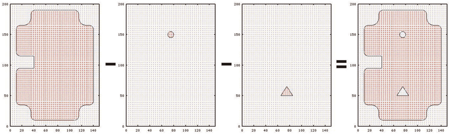
Determination of points belonging to the area in the pocket that has to be machined.

From those points, the distance to every segment in the pocket boundary is calculated using the distance formula, and the shortest distance for each point is selected and stored in a matrix, generating a discretized mesh version of a Voronoi mountain. ²⁰ Figure 2 presents an example pocket and the corresponding Voronoi mountain generated by this method. Every point’s height corresponds to the shortest distance to a pocket boundary; therefore, it corresponds to the largest diameter that can be used to machine a circle using that specific point as a center. This value is called maximally inscribed circle (MIC) by Elber et al. ¹² or LIC by Chen and Fu. ²¹ Equation (1) shows how LIC is calculated for each point within the pocket boundary

$$\text{LIC}(x,y)=\text{min}[\text{dist}(P(x,y),b_1),\text{dist}(P(x,y),b_2)\dots \text{dist}(P(x,y),b_n)]$$

(1)

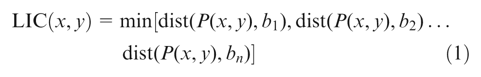
where P(x, y) are coordinates of the considered point and b_n is the portion “n” of the pocket boundary.

Figure 2.

Example pockets and their corresponding Voronoi mountains determined by the method.

Using the Laplacian discrete operator, points near the MA are selected and their x and y coordinates are extracted from this mesh. The Laplacian discrete operator is an isotropic measure of the second spatial derivative and is commonly used in edge detection for image processing, providing a simple measure of the concavity/convexity of the surface. This operator is implemented through a matrix convolution using the following matrix as kernel ²²

$$\nabla =\left[\begin{array}{ccc}\hfill 0\hfill & \hfill 1\hfill & \hfill 0\hfill \\ \multicolumn{1}{c}{1}& \hfill -4\hfill & \hfill 1\hfill \\ \multicolumn{1}{c}{0}& \hfill 1\hfill & \hfill 0\hfill \end{array}\right]$$

This well-known implementation of the operator was selected because it is already available as a function in the used programming language, and it leads to good results in detecting the MA points.

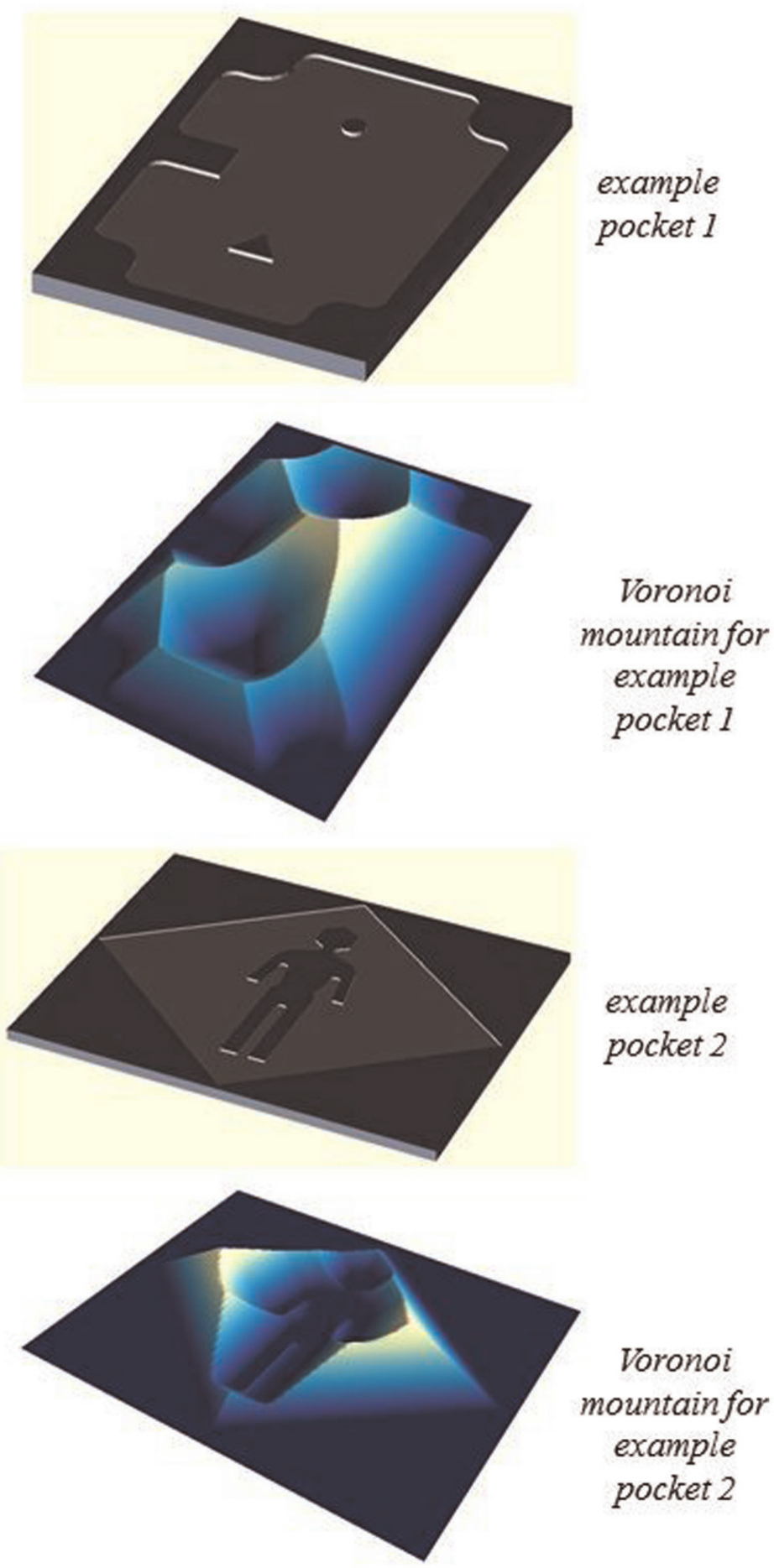
An example of the Laplacian value plotted as vectors for each point in the surface is shown in Figure 3. As seen in this figure, the points that belong to the mountain’s crest have a negative value, and such value leads to the selection of those points.

Figure 3.

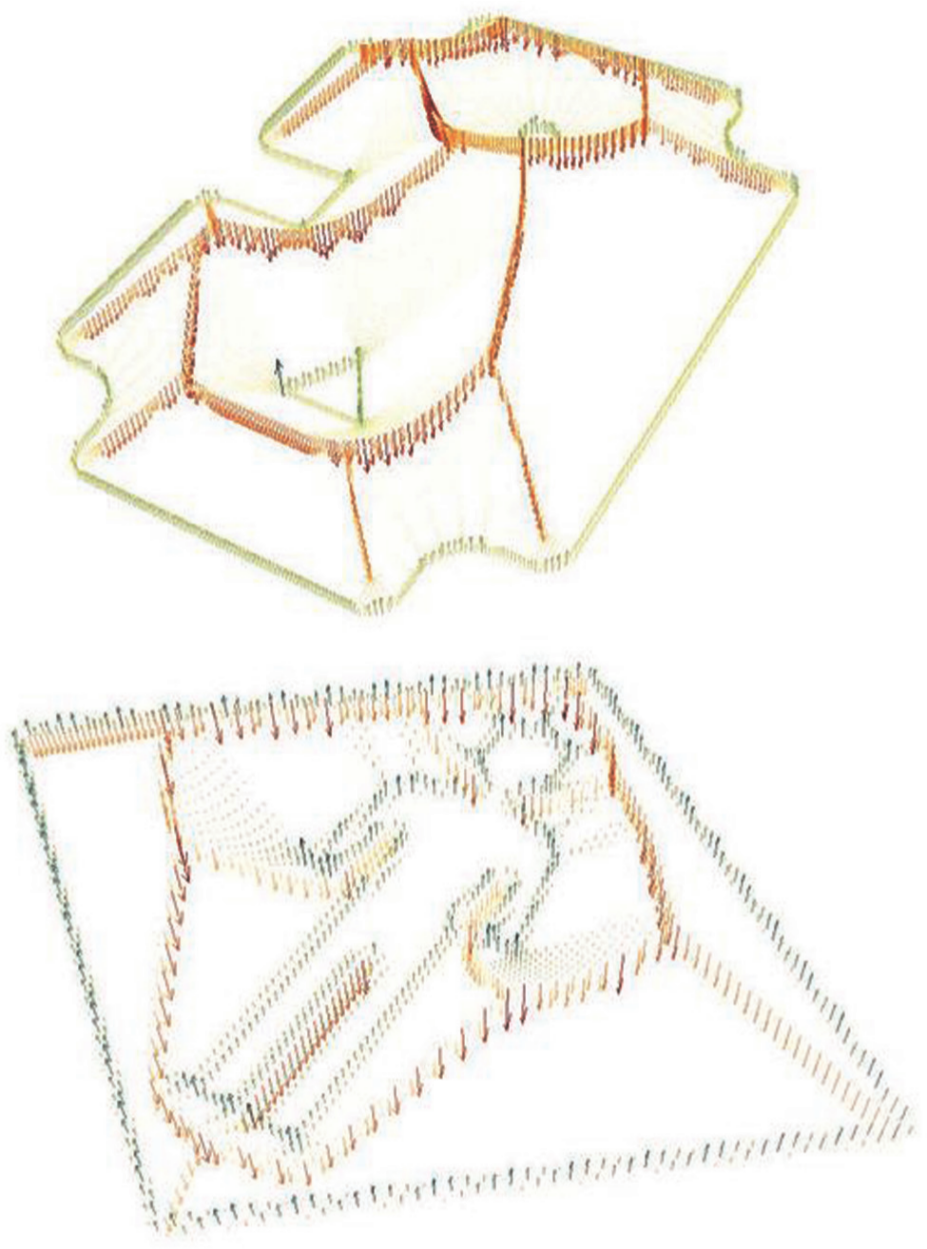
Laplacian value plotted as vectors over the Voronoi mountain.

Since a discretized mesh is used, the resulting points are not necessarily a part of the MA, but they are certainly near to it, and therefore, they need to be adjusted. For this propose, the surface gradient is used, which is a vector that points to the direction of greatest increase of a scalar field. When calculating the gradient of a Voronoi mountain, since the height of the surface represents the distance to the nearest boundary (which is equivalent to the LIC), the maximum slope will be equal to 1, and the gradient will be pointing away from the nearest boundary. The x and y coordinates of the selected point in the mesh can be adjusted by calculating the surface gradient and adding the obtained value to each one of the original coordinates of the point. In Figure 4, a detail of a Voronoi mountain gradient is shown.

Figure 4.

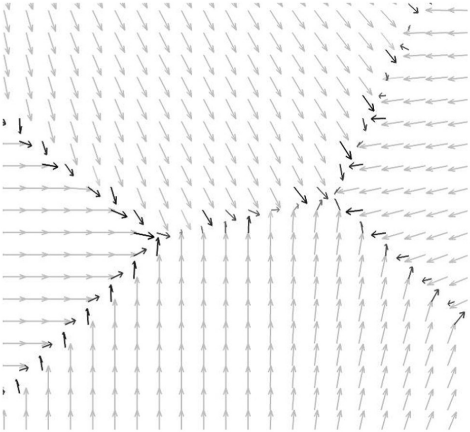
Detail of the Voronoi mountain gradient, where the darker arrows are used to adjust the medial axis position.

The described procedure produces a series of points (x, y, LIC), and examples of the points obtained with this method are shown in Figure 5.

Figure 5.

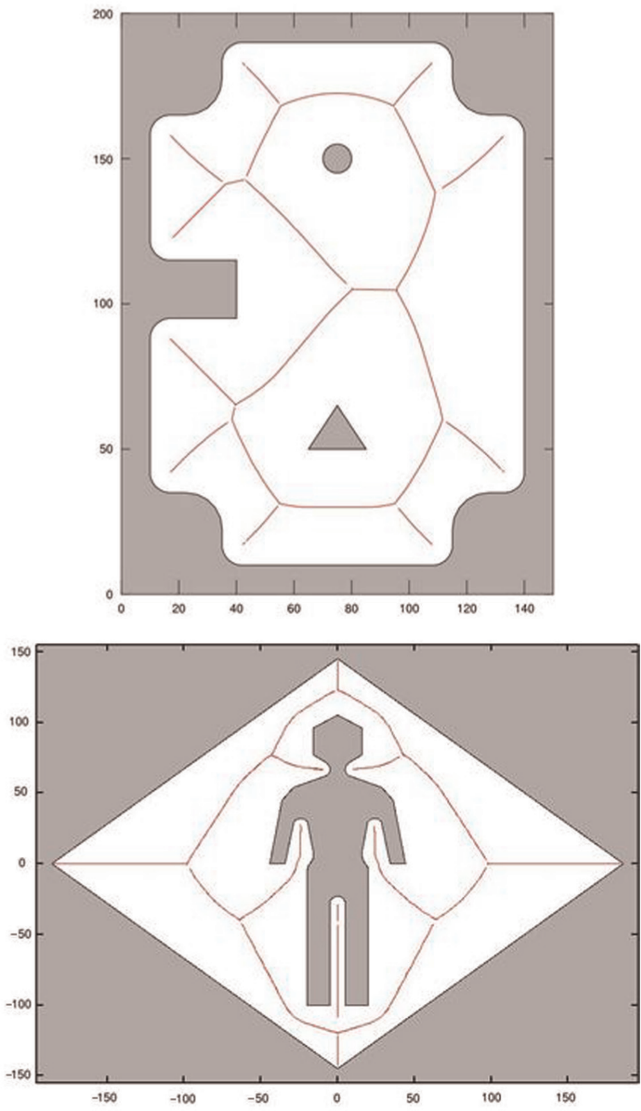
Medial axis points.

The obtained points have to be sequenced before they can be used to generate a tool path. To this end, the distance between each of the points is calculated using equation (2). Starting with the point having the largest LIC value, the points are sequenced selecting always the nearest point

$$\text{distance}=\sqrt{{(x_i-x_j)}^2+{(y_i-y_j)}^2}$$

(2)

where (x_i, y_i) are coordinates of point i and (x_j, y_j) are coordinates of point j.

Analysis of the resulting MA: cutting tool selection and area segmentation

After sequencing the points by distance, the accumulated length (S) corresponding to each point is calculated by equation (3)

$$S_i=\sum _{i=2}^n\sqrt{{(x_i-x_{i-1})}^2+{(y_i-y_{i-1})}^2}$$

(3)

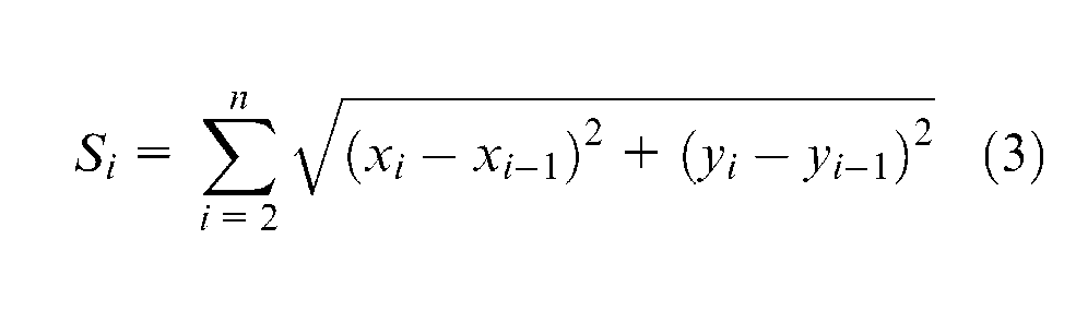
where S_i is the accumulated distance to point i, (x_i, y_i) are coordinates of point i, (x_j, y_j) are coordinates of point j, and n is the number of points.

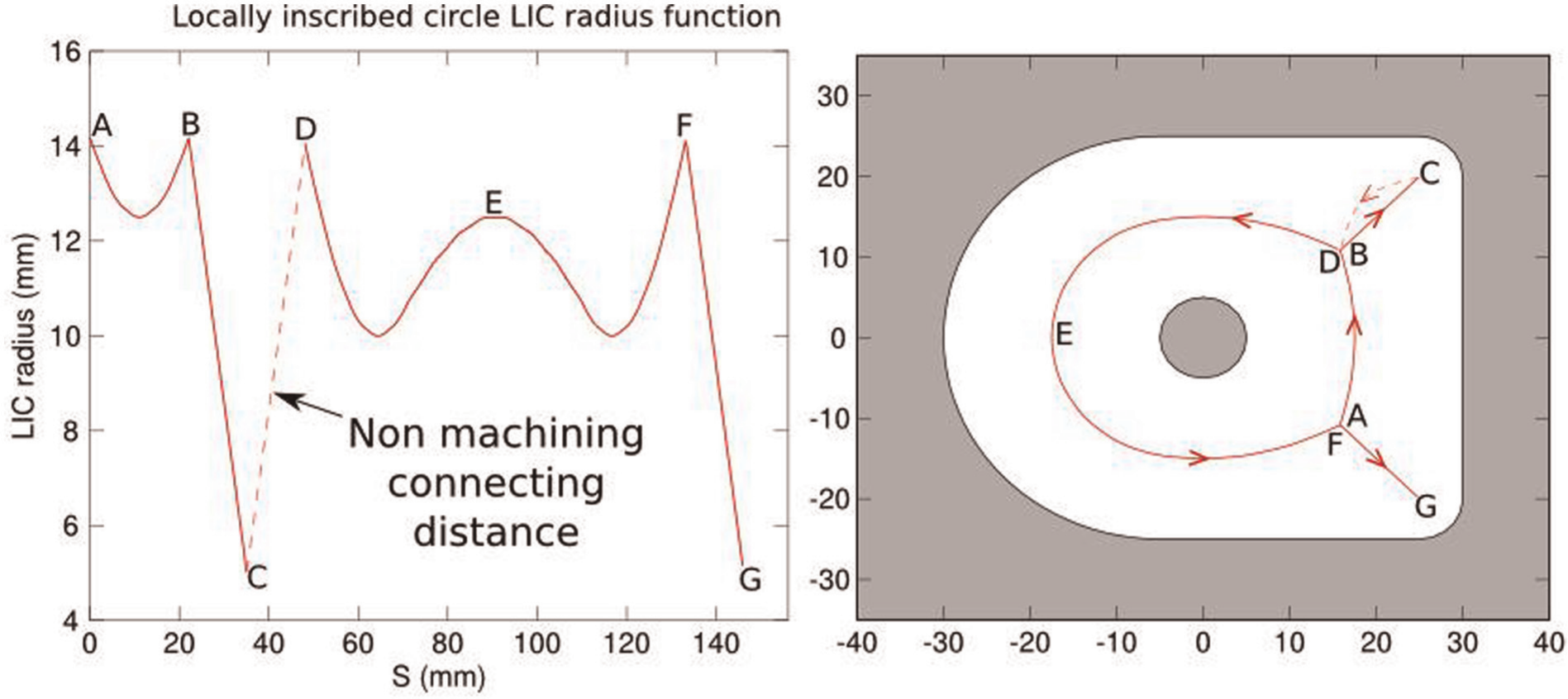
The values (S, LIC) are used to plot a graph (Figure 6) similar to the one proposed by Chen and Fu. ²¹ It should be noted that the LIC graph presented in this work contains all the points of the calculated MA and not just a portion of them, and therefore, it contains intervals of the parameter S that do not have an associated LIC value.

Figure 6.

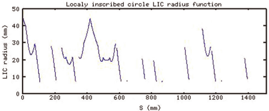
LIC graph.

Some methods have been proposed to perform optimal tool selection.^23–26 Finding an optimal solution to this problem is not simple due to the large amount of variables involved. As proposed by Chen and Fu, ²¹ the LIC graph is used to solve two problems: (a) choose the cutting tools to be used (tool selection problem) and (b) decide which areas can be machined with each tool (area segmentation problem). Although they are different problems, in this work, they are solved in a combined manner.

As a starting point for both problems, the largest and smallest tools for machining the pocket are selected. The largest tool is selected by picking the largest tool available whose radius multiplied by 1.4 is less than the highest value of the LIC. We use the value of 1.4 as a threshold that allows the generation of a TR tool path (see Figure 7). Similarly, the smallest tool diameter is selected based on the minimum value in the LIC graph and dividing it by 1.4. Other tools with radii between those values can be selected as well, but they will be considered adequate depending on (a) the shape of the pocket (and therefore the shape of the LIC graph) and (b) the machining capability (e.g. number of cutting edges, recommended feed rates).

Figure 7.

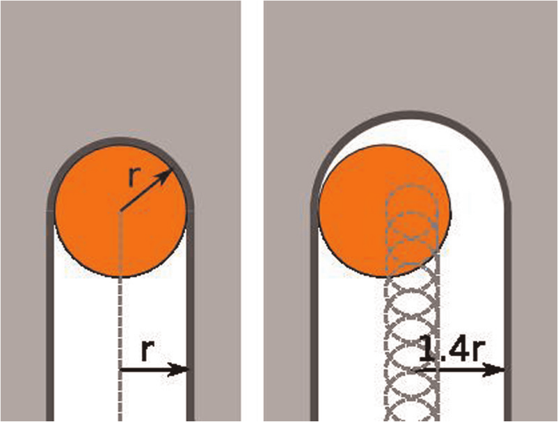
Smallest machinable region using a trochoidal tool path.

The area to be machined is assigned to each tool using the LIC graph as follows:

1. Horizontal lines corresponding to the minimal TR path radius for each tool available are plotted in the LIC graph. Considering that the diameters of the available tools are 10.0, 25.0, and 40.0 mm, three horizontal lines are drawn on the left-hand side of Figure 8, which correspond to the values of 7.0 (i.e. 5.0 mm radius multiplied by 1.4), 17.5, and 28.0 mm, respectively. The medial axes for different tools for the example pocket are shown on the right-hand side of Figure 8.

2. The segments of the MA in between two tools are assigned to the next tool with lower radius. The area assigned to each tool is obtained by drawing a series of circles with their center on selected points along the MA. Each of these points is associated with a radius (which was used to create the MA), and these radii are used to create the circles. The union of the areas of those circles corresponds to the area to be machined by that tool. This process is shown in Figure 9(a)–(f).

Figure 8.

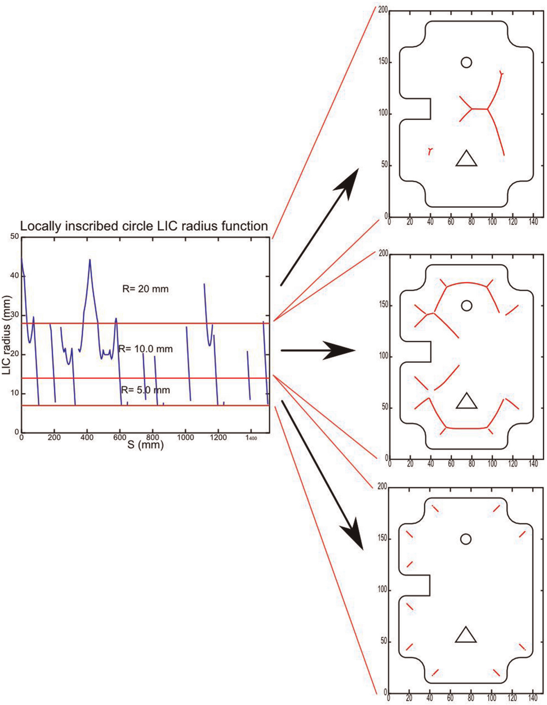
Medial axis division using the LIC graph and the selected tool diameters.

Figure 9.

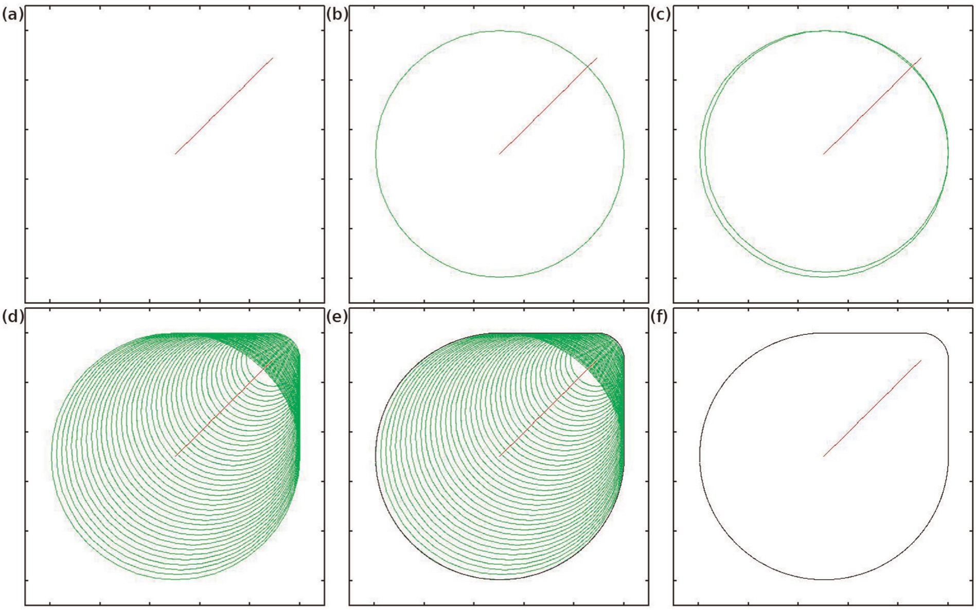
Determination of the area to be machined by a tool, given a medial axis (a) example of MA segment; (b) first circle at the start of the MA; (c) two circles at the start of the MA; (d) all the circles generated along the MA; (e) area generated by the union of the circle’s areas; (f) area obtained for this particular MA.

The next step consists of selecting the tools to be used, in order to minimize the machining time. The following algorithm is proposed for selecting the tools to machine a pocket.

1. The tools are listed (i = 1 … n) in an ascending order according to the tool diameter, where n is the number of available tools.

2. Select tool i = 1 (smallest diameter), and generate its tool path. Using the length of the obtained path and the recommended feed rate, the machining time is calculated. This machining time is usually the longest, and therefore, this value is used as a reference. The tool i = 1 is selected to be used.

3. i = 2

4. The tool paths and their respective machining times are calculated for the following tool combinations:

5. If the machining time is shorter in step 4a compared with step 4b, tool i is marked to be used.

6. i = i + 1; if i = (n − 1), go to step 7, otherwise go back to step 4.

7. In order to decide between the largest tools, an additional test is made, which corresponds to the calculation of the machining times for the following tool combinations:

8. In order to choose among using tool n, tool (n − 1), or both, the shortest machining time is selected and the corresponding combination is used.

As an example of the application of this algorithm, the tool that is initially available is the one with the smallest diameter (tool 1), whose path results in the longest time, since the entire area of the pocket needs to be machined. In the next step, the tool combinations 1–2–3 and 1–3 are considered. If the first combination results in the shortest path, tool 2 is selected, but if the second combination is better, tool 2 is not used.

Assuming that tool 2 is not used, the tool combinations 1–3–4 and 1–4 are considered. If the first combination results in the shortest path, tool 3 is selected, but if the second combination is better, tool 3 is not used.

Supposing tool 3 is used, tool combinations 1–3–4–5 and 1–3–5 are considered. If the first combination is better, tool 4 is selected, but if the second combination is better, tool 4 is not used. The following steps would be similar to these, until all available tools are taken into account.

This method allows finding the shortest machining time performing 2 ×n tests, while by testing all the possibilities, it would take 2 ⁿ tests. Using this method with six different tools (diameters = 40, 32, 20, 14, and 10 mm), the best sequence was 32–20–10 mm. This tool sequence and other sequences that generate the shortest machining times, as well as the times for some CP trajectories, for the presented pocket are shown in Figure 10. Also, as a reference, the times for only one tool (CP-10 and TR-10) were included.

Figure 10.

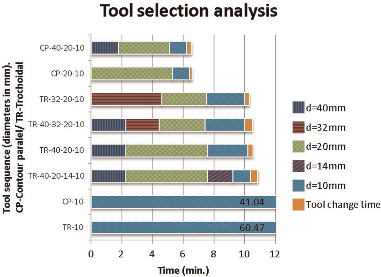
Different tool sequences and their corresponding machining times.

Circular model TR tool path generation

After the tools are chosen and the sequence of points is divided into machinable segments for each tool, then the complete tool path is generated. A helical ramp is programmed in the first point of the sequence, which corresponds to the largest LIC. As it reaches the desired axial depth of cut (a_p), the tool then moves along a circular path such that the circle radius is equal to the LIC value at that point. After that, the algorithm moves along the points in the sequence, and when the desired radial depth of cut is attained, a circular path is programmed to generate a circular tool path segment (Figure 11).

Figure 11.

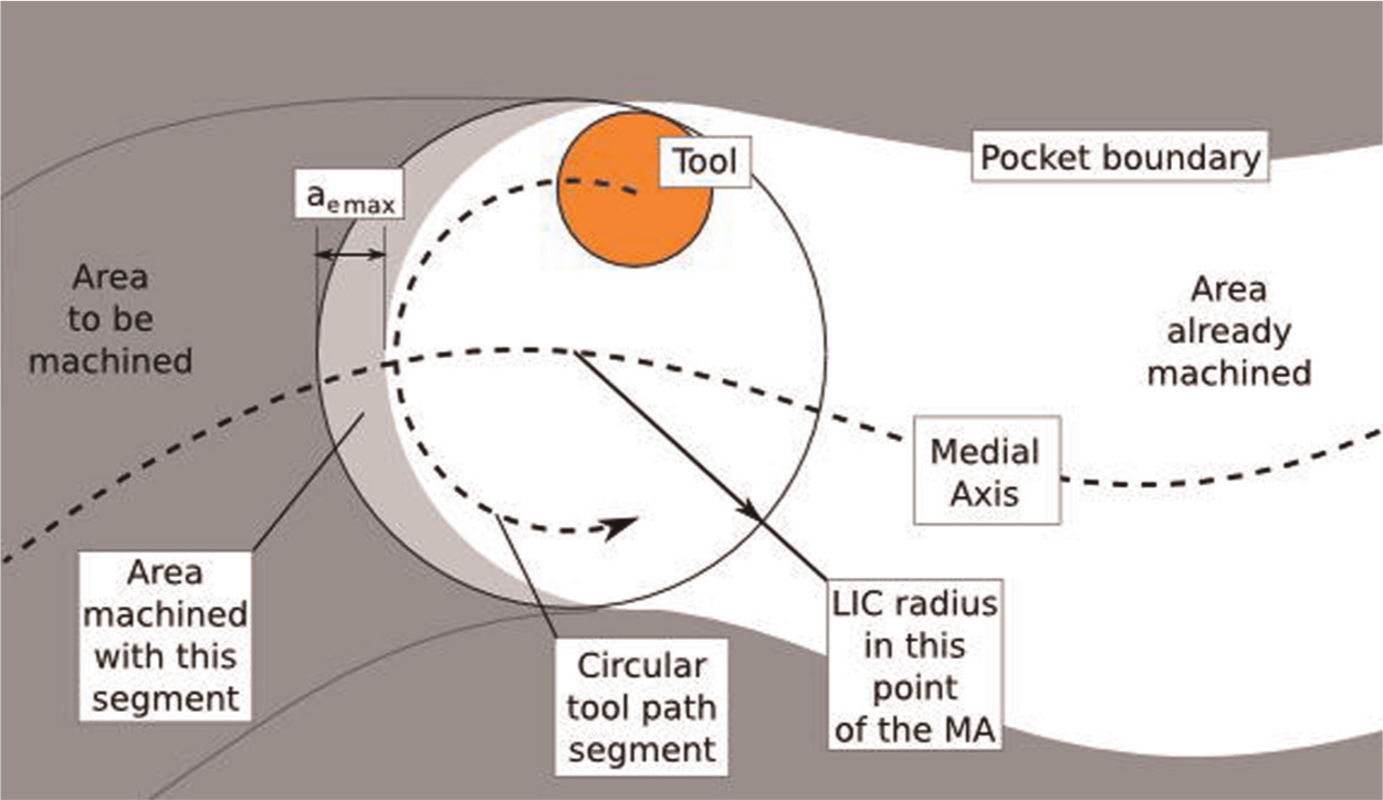
Circular mode tool path generation.

Although some simple pockets have an MA with one segment, in general, the MA will have discontinuities (Figure 12). At those points, the tool must be retracted, and in some cases, a new helical ramp is needed.

Figure 12.

Discontinuities in the medial axis for a pocket.

Pixel-based analysis

Although the generated tool path completely removes the material of the pocket, it will be very long because every trochoid cycle performs some idle cutting. As proposed by Ibaraki et al., ⁵ in order to shorten the TR path, a straight line is used to connect arc segments, and consequently, the machining time is reduced.

There is another situation where idle cutting takes place, and it occurs when two of more branches of the MA occur near one another (Figure 13). In this case, one of them is chosen first, and the area inside the circle will be machined, and when second branch is started from that nearby point, most of the material will have already been removed, resulting in idle cutting.

Figure 13.

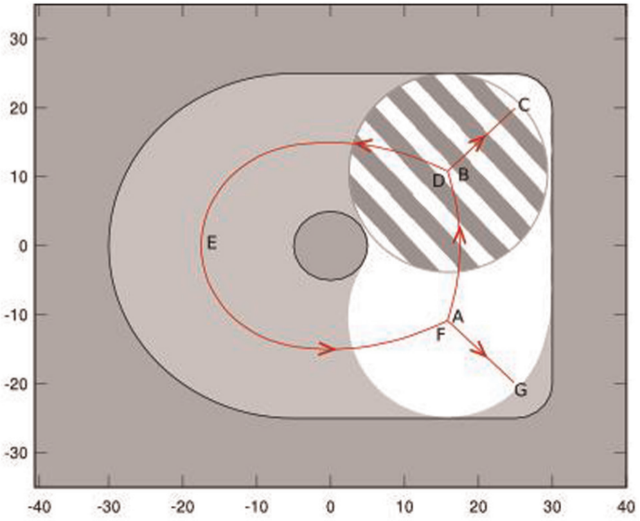
The circle to be machined centered in point D of the medial axis was previously machined when centered in point B, and therefore, it does not need to be machined again.

To overcome those limitations, a simple pixel-based Boolean simulation of the machining process was implemented. This method generates and stores information about the stock removed in each movement. This information allows reducing the path’s length, using precise start and end points (or angles) for each calculated arc. It also avoids the helical ramp strategy when the material has already been removed, provided an empty space exists for the tool to descend.

In order to implement this pixel-based simulation, a mesh composed of squared pixels is generated (Figure 14). Each of the pixels of the generated mesh can have “unmachined” or “machined” states, and they all are marked as “unmachined” when the process starts. When the software generates a circular segment of the tool path, the machined area is determined, and the points whose x and y coordinates are within the machined area are marked as “machined.”

Figure 14.

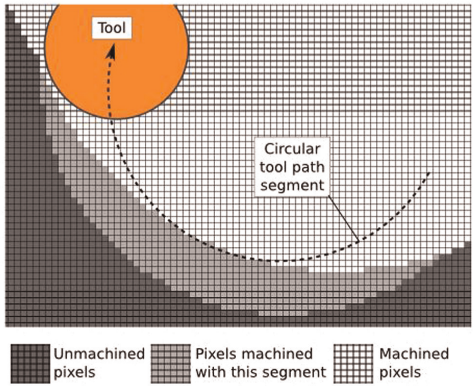
Pixel-based simulation.

The analysis can also be used to minimize the tool retractions when the connecting path between the circular machining segments moves through areas where the material has already been removed. Also, using this pixel-based procedure allows the MA to be considered as a whole, avoiding the need to make any specific geometrical or topological analysis. Finally, the pixel-based analysis is used to generate a looping tool path in the corners of the pocket, similar to the procedure proposed by Choy and Chan ²⁷ and Banerjee et al. ⁷ (Figure 15).

Figure 15.

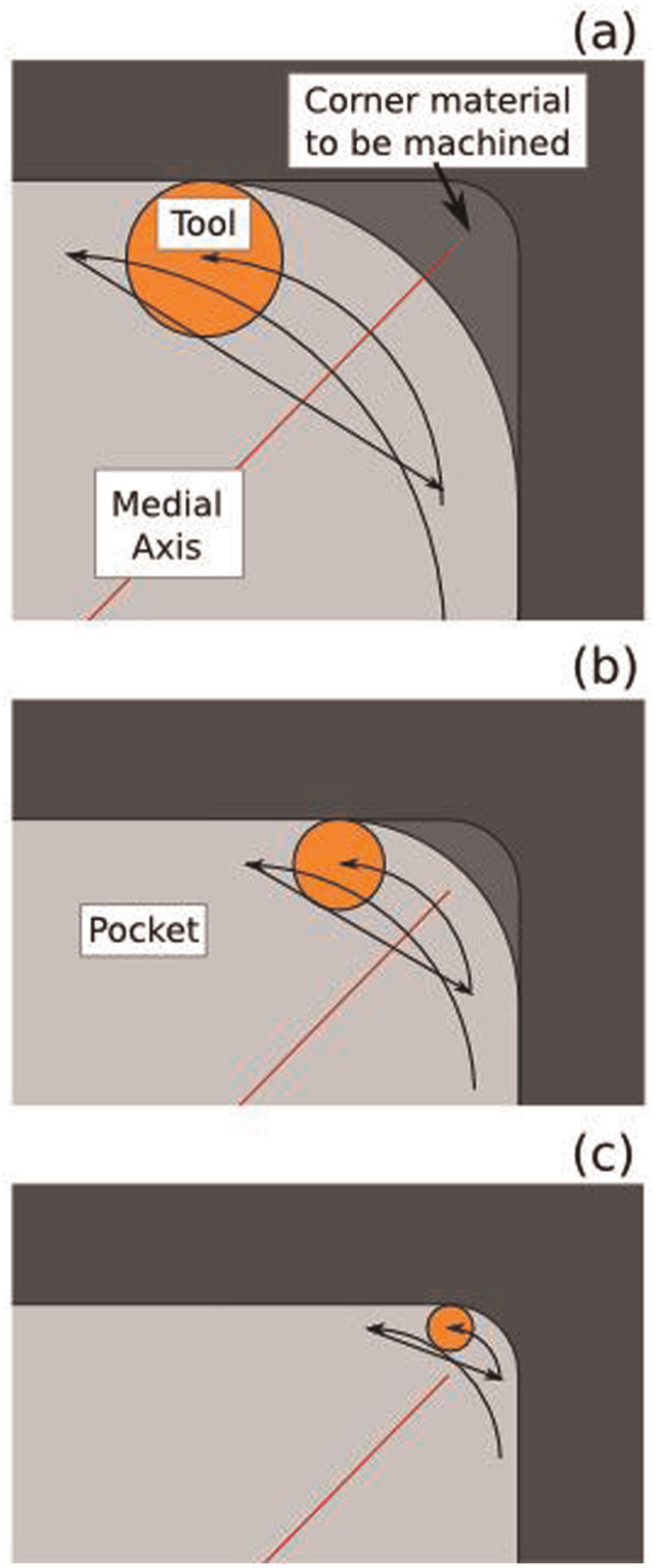
Automatically generated path sequences for machining the corner of a pocket with different tools (a) larger diameter tool; (b) medium diameter tool; (c) smaller diameter tool.

Implementation and results

The presented method was implemented in the GNU Octave language. ²⁸ Octave is an open-source high-level interpreted language, primarily intended for numerical computations. Each pocket area was discretized obtaining a matrix with 400 elements in the longest side. The number of points of the MA and the computing time depends on the complexity of the pocket polygons. Using a computer with a dual-core 1.6-GHz processor, the central processing unit (CPU) time for calculating the MA varies between 20 s with a polygon formed with 40 segments and 70 s in a polygon with 260 segments.

Using the MA, cutting tools, and process data, standard G-Code (International Organization for Standardization (ISO) 6983) generation was implemented in the same language. In this case, the computing time depends on the complexity of the pocket and the tool diameter, taking more time with smaller diameter tools. The resulting tool path for a test pocket is shown in Figure 16, whereas the machined volume is shown in Figure 17. The execution time to generate these paths was equal to 150 s in the same computer. Other pockets and the generated tool paths are shown in Figures 18 and 19.

Figure 16.

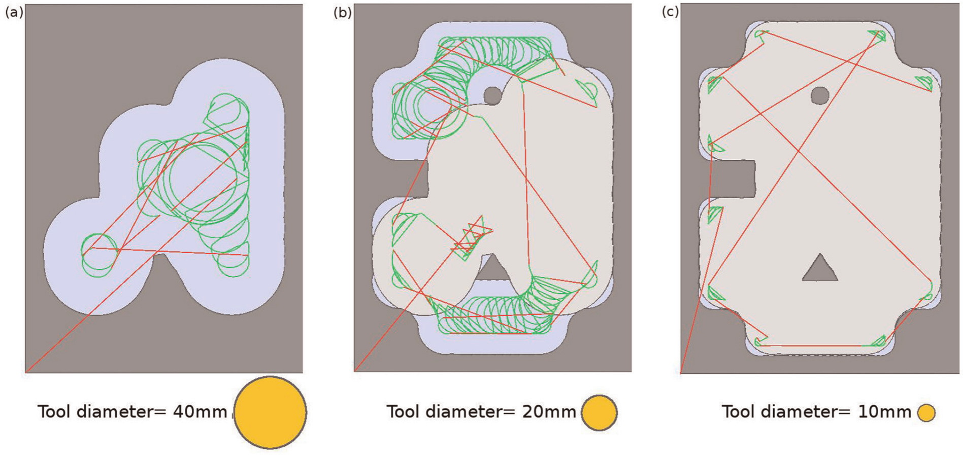
Generated tool path using tools with (a) d = 40 mm, (b) d = 20 mm, and (c) d = 10 mm.

Figure 17.

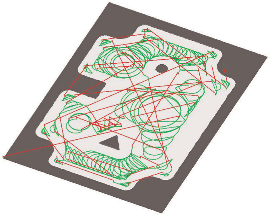
Resulting simulation of the removed material (all the pocket material was effectively removed).

Figure 18.

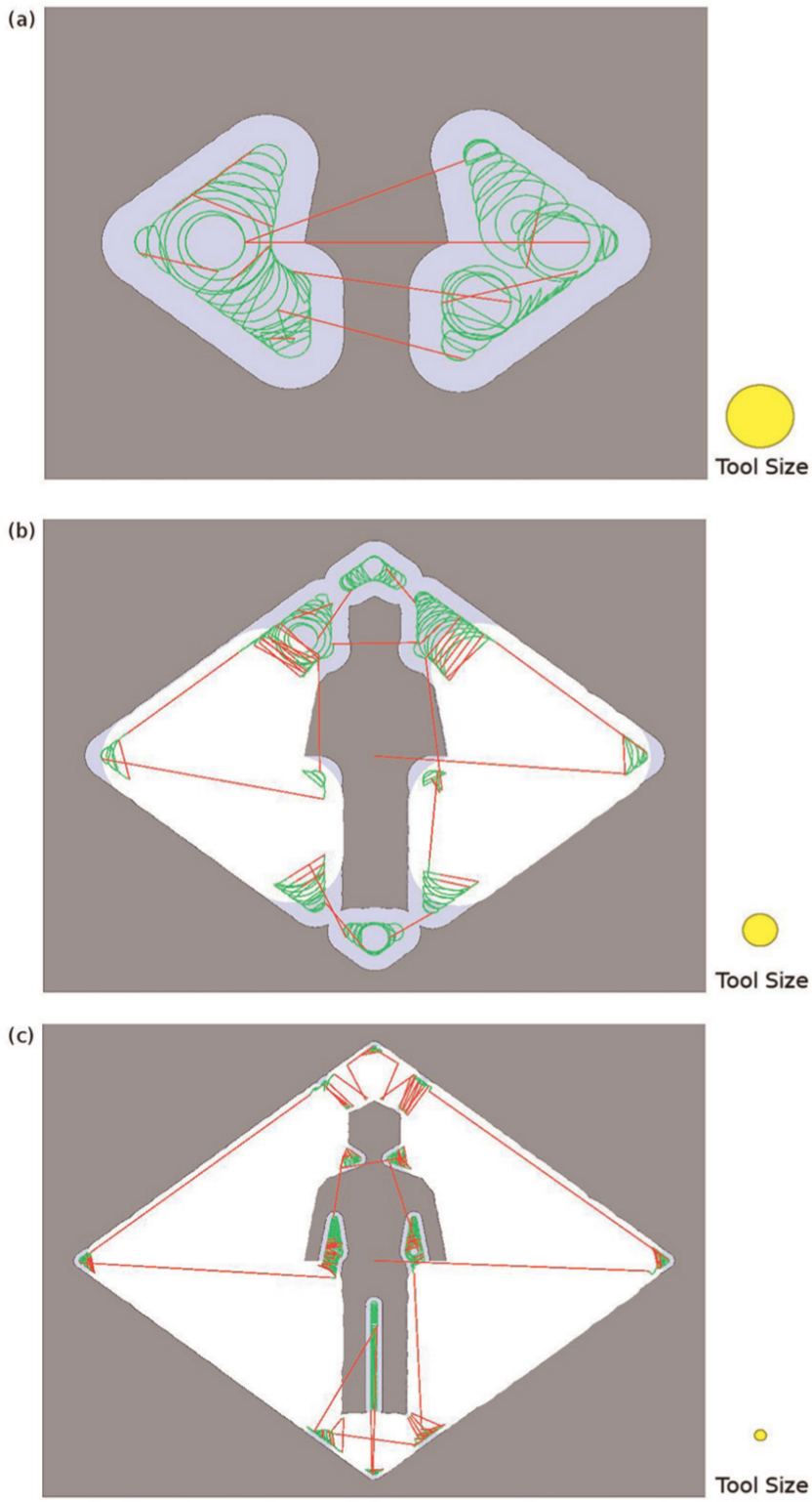
Generated tool paths for machining an example pocket with an island similar to a human being (three cutting tools) (a) larger diameter tool; (b) medium diameter tool; (c) smaller diameter tool.

Figure 19.

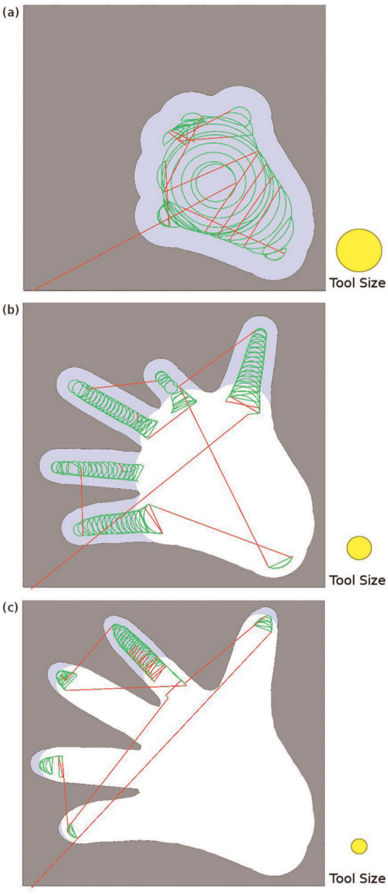
Generated tool paths for machining an example pocket similar to a hand (three cutting tools) (a) larger diameter tool; (b) medium diameter tool; (c) smaller diameter tool.

The use of traditional tool path strategies such as CP or direction-parallel paths results in momentary increments in radial depth of cut, which take place in the corners. Such increments are problematic when machining hard materials or when HSM. On the other hand, the proposed method seeks to avoid these momentary increments in the radial depth of cut, allowing the use of larger feed rates, compensating the lengthier paths. For example, the two graphs shown in Figure 20, which were determined in this work, represent the momentary ratio between the radial depth of cut a_e and the tool diameter d along a tool path. Figure 20(a) shows the ratio a_e/d for the TR tool path in Figure 16(b), whereas Figure 20(b) shows the ratio a_e/d for a CP tool path machining the same area (Figure 21). It can be noticed in Figure 20 that in the CP tool path, the tool is frequently fully immersed in the material of the part (i.e. a_e = d), which leads to an increase in cutting temperature, whereas in the TR path, the largest value of the ratio a_e/d along the whole path is 0.4.

Figure 20.

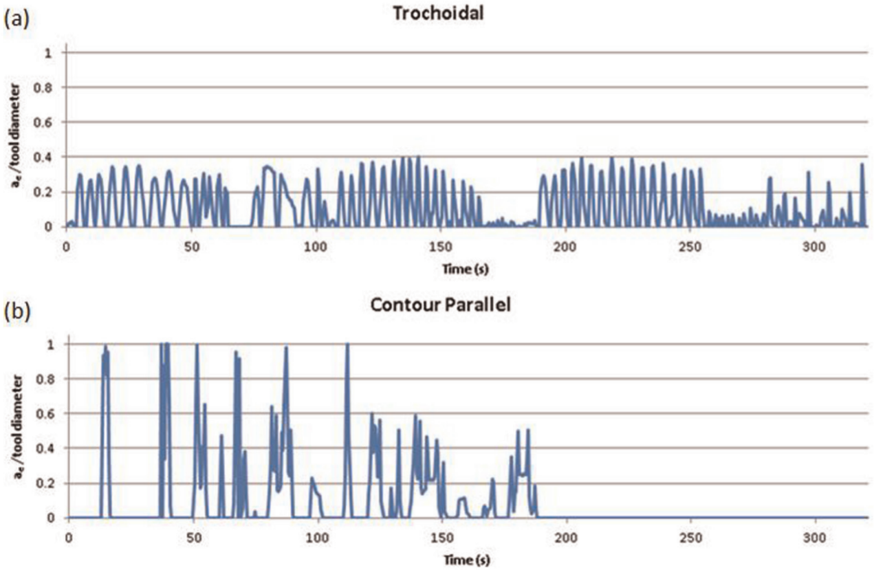
Momentary ratio between the radial depth of cut a_e and the tool diameter d along the (a) trochoidal and (b) contour-parallel tool paths.

Figure 21.

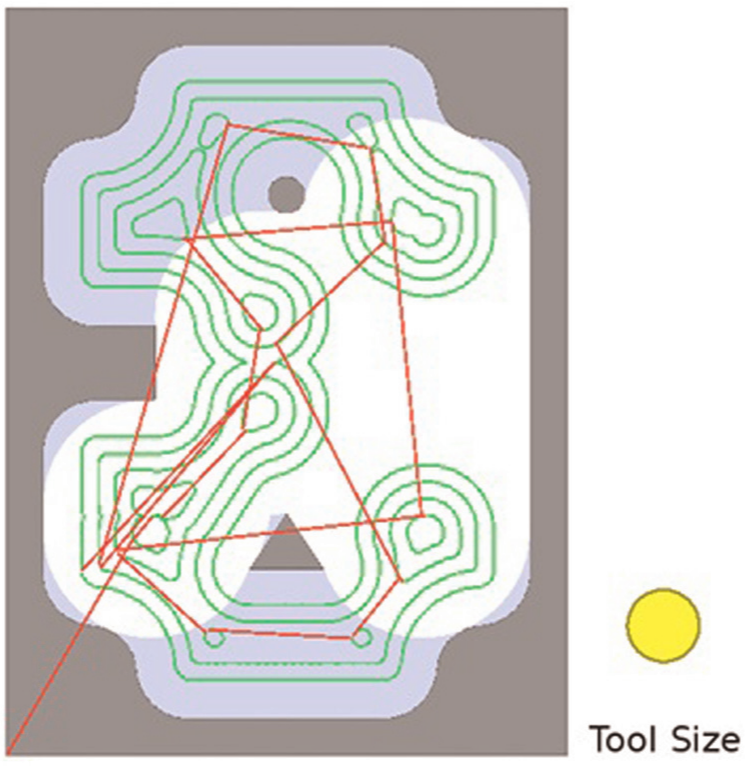
Contour-parallel tool path generated for the pocket in Figure 16.

Conclusion

This article presented a method to generate tool paths for machining 2½D pockets with or without irregular shapes (i.e. irregular straight and curved segments), which may contain islands. It considers the use of milling cutters with different diameters for the machining of a pocket, and for each chosen tool, the method attempts to generate TR paths from the MA. Finally, the generated TR path is adjusted through a pixel-based procedure in order to reduce the time in which the tool performs idle cutting.

Usually the length of the tool path resulting from the proposed algorithm is larger than the lengths obtained from CP (as shown in Figure 10) or direction-parallel paths, mainly because in those strategies, the radial depth of cut is maintained constant most of time, whereas in a TR path, this value is constantly varying from zero to a maximum and back to zero again. However, in traditional tool path strategies, momentary increments in radial depth of cut place in the corners, which can lead to problems when machining hard materials or when HSM. Such momentary increments in the radial depth of cut do not occur in the TR tool path, and thus larger feed rates may be used.

In a future work, we intend to investigate the use of the TR tool path generated by the proposed method in the machining of parts, and larger feed rates than those commonly used in CP paths will be tested. The proposed tool path with the respective cutting conditions will be evaluated regarding the accuracy of the parts and tool wear.

In the generated TR tool path, some idle cutting takes place, because of the connection between every circular tool path with the next. This limitation can be avoided in future developments, using alternating climb and down milling, or optimizing the sequence of the circular segments in order to minimize the tool travel segments.