Sage Journals: Discover world-class research

Abstract

In this study, magnetic abrasive finishing, a polishing method using novel bonded magnetic abrasive particles, is implemented in the nanometer-scale surface polishing of STAVAX (S136) die steel workpieces, which are widely used for precision lens molds. With the aid of run-to-run control, a process control method, nanometer-scale mold surface quality is achieved and maintained over multiple runs. A specially designed magnetic quill equipped with an electromagnet was connected to a computer numerical control machining center to construct the polishing setup. Based on Preston’s equation and a set of preliminary experiments, design of experiment and analysis of variance were used to select and evaluate the relevant control parameters for the process. The finishing results show that the magnetic abrasive finishing has a nanometer-scale finishing capability (down to 8 nm surface roughness). Under run-to-run control with the selected parameters, the surface roughness values were successfully maintained below the target values (10 and 50 nm for R_a and R_max, respectively), which shows that the proposed magnetic abrasive finishing scheme is readily adaptable to ultraprecision polishing applications, which are subject to disturbances for a relatively long period of time.

Keywords

Magnetic abrasive finishing bonded abrasive particle run-to-run control ultraprecision mold surface finishing design of experiment

Introduction

The demand for ultraprecision optical parts has rapidly increased in recent years with the advent of the optoelectrical industry. The development and implementation of highly precise finishing methods are essential to the manufacturing of such sophisticated parts. For example, aspherical lenses are commonly produced in volume by injection molding. Because the geometric characteristics of the mold surface are directly transferred to the lens surface, the selection of the surface finishing technique for the three-dimensional mold, which is most often simply polishing, is a critical factor in determining the quality of the final lens product.¹

Moreover, because a surface roughness on the nanometer scale is required for the majority of optical products available nowadays, it is necessary to develop an even more precise polishing technique. It is difficult to achieve high surface quality for parts with three-dimensional shapes with conventional polishing methods such as lapping and chemical mechanical polishing (CMP) because they are best suited for flat surfaces. Several nontraditional techniques, including electrolytic polishing and electrolytic in-process dressing (ELID) grinding, have been pursued as ways to finish free-form lens mold surfaces. However, the fabrication of appropriate consumables such as electrodes and grind wheels for specific part shapes remains both challenging and expensive.

A more recent approach to solving the above-mentioned problems is to utilize functional fluids combined with loose abrasive particles. Kuriyagawa et al.² performed a study on lens polishing using electrorheological (ER) fluids, the viscosity of which increases proportionally to the strength of an applied electric field. Zhang et al.¹ extended the use of this polishing method to conductive materials such as tungsten carbide. Generally speaking, however, ER polishing has some intrinsic weaknesses such as a low polishing force and the difficulty involved in selecting appropriate abrasives.

Magnetorheological (MR) fluids, which undergo significant changes in both mechanical and optical properties upon the application of a magnetic field,³ are also used to polish and finish part surfaces.⁴ Although MR finishing has shown precise finishing capability,⁵ the low material removal rate (MRR) and difficulty in process control because of the complicated process characteristics are the main concerns for this process.

Magnetic abrasive finishing (MAF), a relatively new technology that uses abrasive particles as a flexible finishing tool, surrounded by magnets that generate a magnetic field around the polishing area,⁶ has recently drawn attention as another potential finishing technique. Yamaguchi and Shinmura⁷ applied MAF to polish the inner surfaces of the tubes and observed the subsequent microscopic changes in surface texture. Jain et al.⁸ investigated the performance of magnetic abrasive polishing (MAP) using loosely bonded abrasives while varying the gap and rotating speed process parameters. Later,⁹ they performed MAF modeling and simulation work and published it along with detailed descriptions of its surface finishing capability. Chang et al.¹⁰ used unbonded abrasives to polish cylindrical parts and analyzed the effects of such process variables as particle size, workpiece hardness and process time on the part surface roughness and MRR. Yin and Shinmura¹¹ presented the application results of vibration-assisted MAF to three-dimensional microscale surfaces. Lin et al.⁶ carried out experiments and analysis with sintered abrasives using the Taguchi method to optimize the process parameters for MAF. Because the finishing characteristics of MAF are closely related to the abrasive particles employed,¹⁰ the development of appropriate abrasive particles for selective finishing has also been investigated.^12,13 Recently, Oh and Lee¹⁴ performed in-process monitoring experiments for MAF using acoustic emission and force sensor signals.

As demonstrated in the literature discussed above, the main concern of recent MAP studies is an effective process control method to allow the efficient application of abrasive particles. In this research, an MAF process is implemented using novel magnetic bonded abrasive particles to allow ultraprecision surface polishing. The achievement and maintenance of a nanometer-scale mold surface is pursued with the aid of a run-to-run (RtR) process control method. Design of experiment (DOE) and analysis of variance (ANOVA) techniques were applied to select and evaluate the control factors (polishing parameters) that dictate the surface roughness of workpieces in polishing experiments.

MAP process

Magnetic abrasives

During MAF, magnetic and abrasive particles are most often applied as a mixture to generate the magnetic field–assisted abrasion. However, when polishing complicated shapes or partially polishing a part, some problems are possible. As shown in Figure 1(a), abrasive particles have a tendency to move down (which has a relatively lower magnetic flux strength) and to gather at the edge under the influence of the centrifugal force imposed by the rotation of the quill. If the quill is then moved, abrasive particles can drop out of suspension, causing serious deterioration in the polishing efficiency. To solve this problem, the abrasive particles can be bonded around the magnetic particles.¹⁵

Figure 1.

Comparison of magnetic abrasive particle types: (a) free abrasive and (b) bonded magnetic abrasive.

The result, as shown in Figure 1(b), is that the abrasive particles are distributed evenly over the workpiece with an increased cutting ability. The advantage of the suggested method over conventional methods has also been verified experimentally.¹²

A cyanoacrylate-based bonding agent (binder) was used to attach the abrasives (diamonds) to the magnetic particles (carbonyl iron particles); this overcomes the magnetic weakening and complicated bonding processes that are a result of the existing bonding methods, such as plasma melting and sintering.^10,13 In addition, a mechanical alloying method, capable of manufacturing smaller magnetic abrasive particles with well-controlled sizes in the micron- to nanometer scales, was developed and applied.¹⁶Figure 2 shows the particles fabricated for this study by the binder and the mechanical alloying methods. The bonded (magnetic and abrasive) particles synthesized by the above-mentioned methods are in ideal shapes, in which one magnetic particle is surrounded by several abrasive particles without a loss in magnetism.

Figure 2.

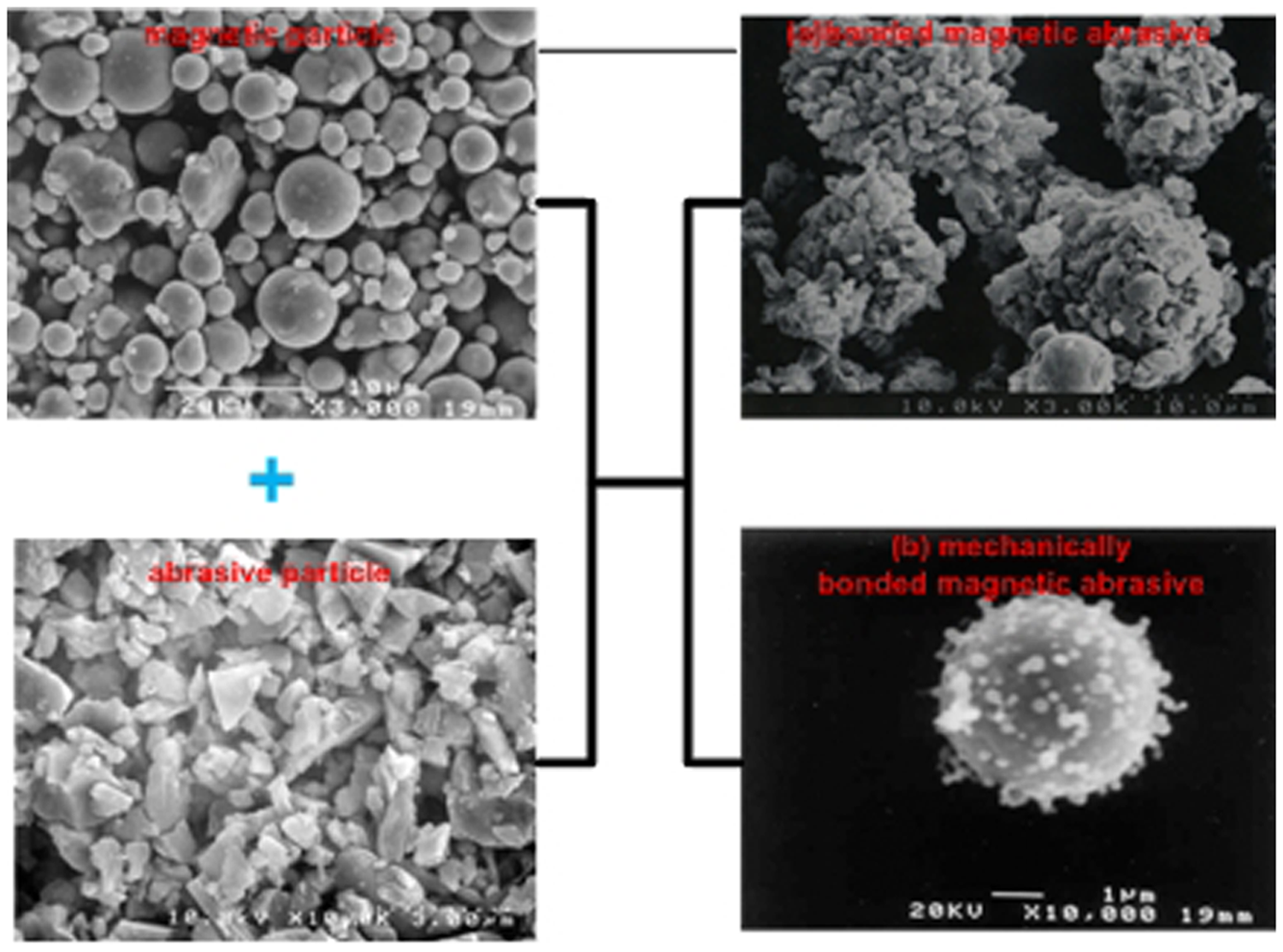
SEM images of magnetic abrasives.

Polishing mechanism

Figure 3 details a schematic of the polishing process using bonded magnetic abrasives. Upon magnetization by the magnetic polishing head, the magnetic abrasive particles are aligned by the quill into chain-like structures. The aligned particles, which are supplied through the gap between the end of the quill and the workpiece as a slurry, act as flexible polishing tools. The polishing area is thus between the workpiece and the quill.

Figure 3.

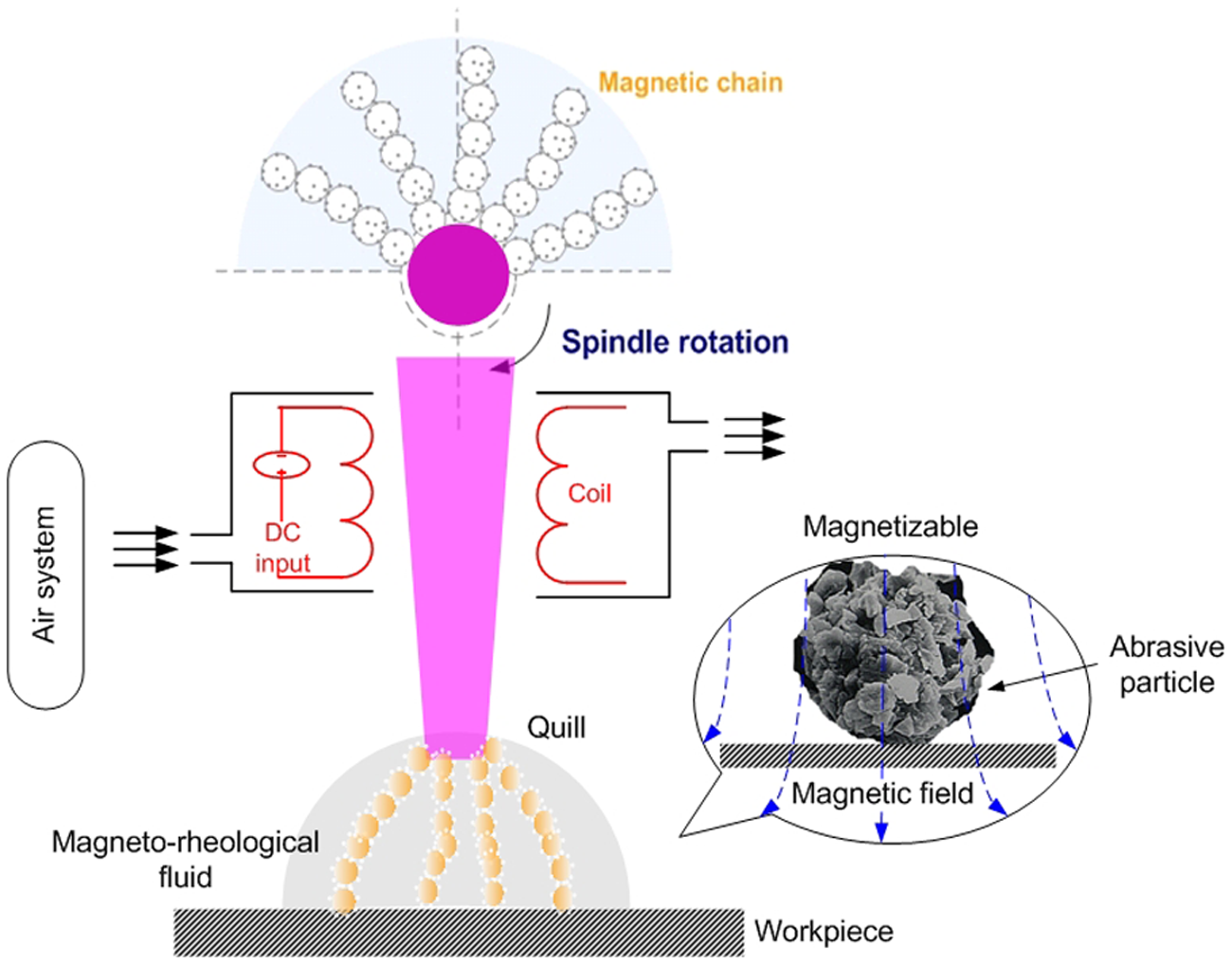
Schematic of polishing process.

In the polishing area, magnetic abrasive particles are in contact with the workpiece because of the normal force from the magnetic field. At the same time, the shear force from the quill rotation causes scratching on the workpiece surface, which is the mechanism for polishing. An electromagnet was used for the magnetic polishing head to generate the normal force; the core of the electromagnet acts as the polishing quill.

The Preston equation¹⁷ is widely used to model the mechanical material removal in loose abrasive processes. The Preston model predicts that the volumetric removal rate at a point P on a workpiece is proportional to the normal load and the relative velocity

\frac{Δ h}{Δ t} |_{P} = C \frac{Δ L}{Δ A} \frac{Δ s}{Δ t} |_{P}

(1)

where h is the depth of wear, A is the contact area, L is the total normal load, C is Preston’s coefficient, s is the sliding distance, and t is the processing time. Preston’s coefficient, C, is a proportionality constant that depends on factors such as the quill conditions, the properties of the abrasive particles and slurry, and the material properties of the workpiece.

Figure 4 shows the preliminary experimental results for a heat-treated steel SKD11 workpieces, which are widely used for lens moldings. The graphs illustrate the normal force measured with a Kistler 9257B tool dynamometer according to variations in the gap size and the size of the bonded magnetic abrasive particles. As shown in Figure 4, the normal force increased with increased abrasive size for a given gap size and had an inverse proportionality with the gap size for a given abrasive size. The effectiveness of the polishing process (via increased normal force) can thus be improved by controlling the gap and the particle size. However, deterioration of the workpiece surface caused by excessive normal force (and excessive abrasive particle size) should be avoided.

Figure 4.

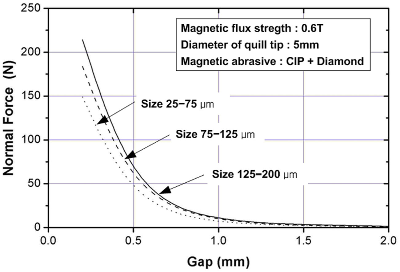
Measured normal load acting on the surface.

Experimental setup

The uniformity of the magnetic flux density distribution between the polishing quill and the workpiece is another important factor for the improvement of polishing efficiency. The strength of the magnetic flux from the magnetic polishing head should therefore be controlled within certain set limits. In order to generate a uniform magnetic field, an electromagnet was used in this study to supply a constant electric voltage and current (50 V and 5 A, respectively). The gaussmeter reading (magnetic flux density) at the end of the quill was approximately 0.6 T. To avoid electromagnet performance losses caused by heat generation after extended use, a cooling device using compressed air was added to the electromagnet setup.

The electromagnet was attached to a machining center to make the polishing setup (Figure 5). In order to prevent particle slippage and to improve polishing performance, a cruciform groove was carved at the tip of the quill. A medium carbon steel SM45C, which has good magnetization properties, was selected as the quill material, and aluminum was used for the rest of the parts. Additionally, a plastic bearing was installed to minimize the magnetic field leakage as the quill rotates.

Figure 5.

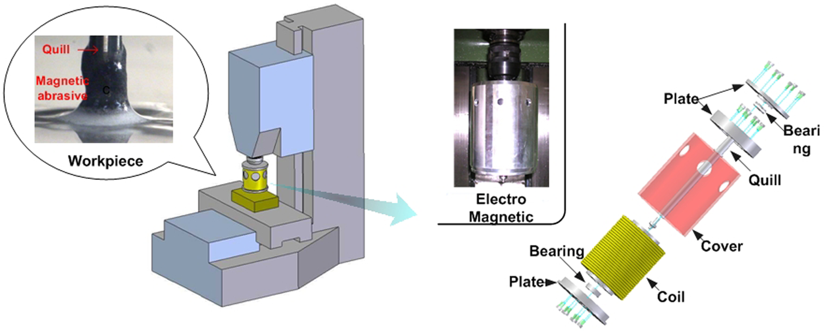
Proposed polishing setup with an electromagnet.

Stainless steel alloy STAVAX S136, which is widely used for precision lens molds, was selected as the workpiece material.

Process analysis using DOE

DOE

To evaluate the effects on performance of several different parameters at a time (e.g. polishing parameters on the surface roughness), a specially designed experimental process is needed. The selection of design parameters and their values should be such that the parameters effectively reflect the effects of physical experimental conditions on characteristic values. In addition, parameter values should be selected as wide as possible to ensure stability in parameter design.¹⁸ After the selection, an appropriate orthogonal array should be chosen for the designed experiments. The orthogonal array is an approach widely used in DOE to make process improvement decisions with the minimum amount of experimental data, using a fractional–factorial approach when there are several factors (parameters) involved. This array represents a way of conducting the minimum number of experiments that would ultimately yield the full set of variables to affect the output performance.

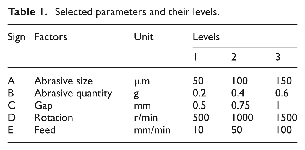
From the Preston equation and the preliminary experiments illustrated in Figure 4, the appropriate process parameters were selected. First, because the normal force is a primary factor in the polishing process, the process conditions relevant to the normal force, such as the particle size, abrasive quantity, and gap size, were chosen as factors. In addition, revolutions per minute (RPM) and feed rate, which influence the shear force, were selected as other factors. The parameter levels were also determined from the preliminary experiments.

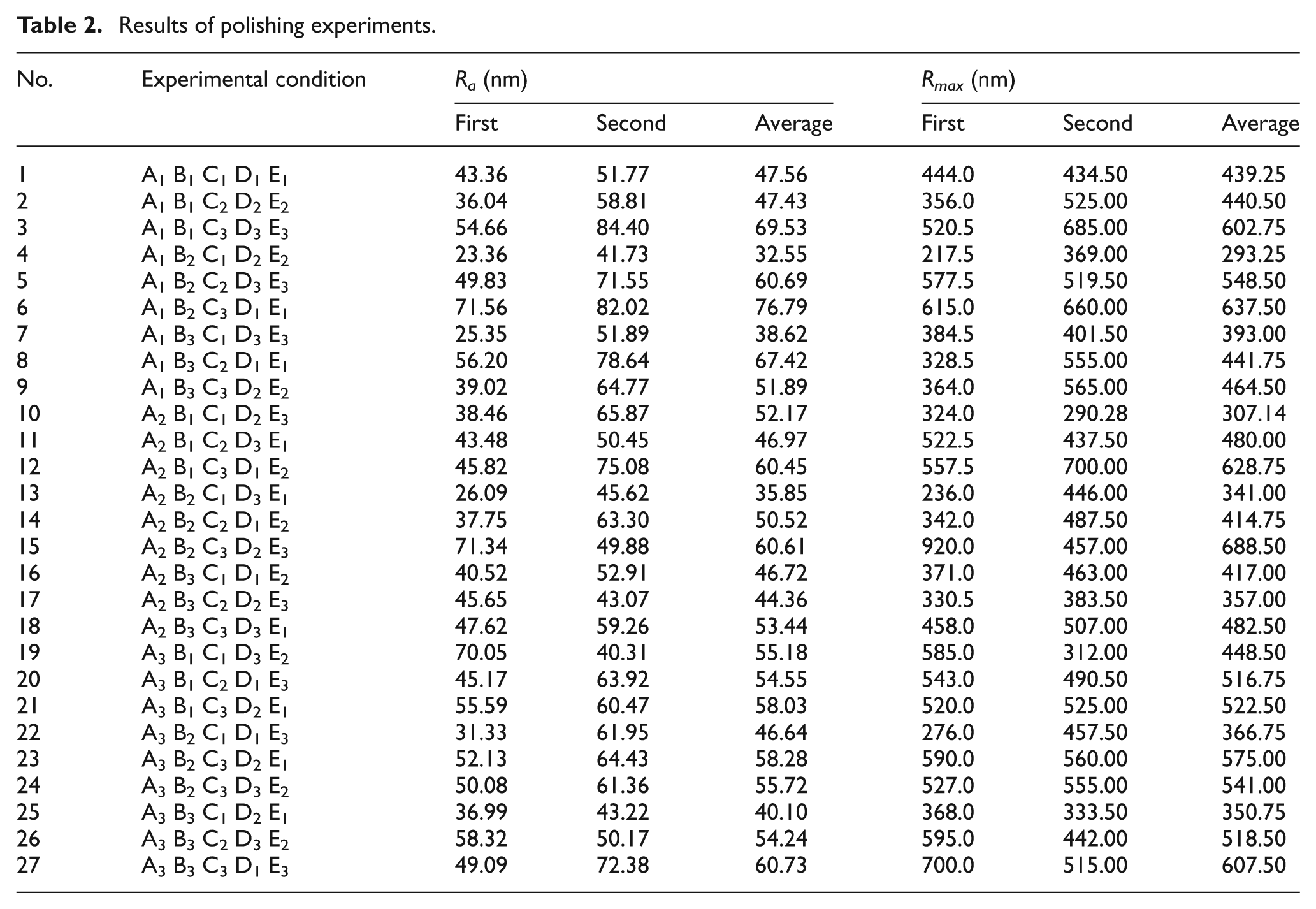
The selected factors and their levels (five factors and three levels of each) are shown in Table 1. Considering the three interaction effects, A × B, A × C, and B × C, the total degrees of freedom of the experiments is 22. As a result, a three-level orthogonal array L₂₇ (3¹³) was selected. The arrangement of the factors for the orthogonal array (Table 2) was chosen according to the linear graph (Figure 6). The polishing experiments were performed in random order twice for each condition according to the designed table of orthogonal arrays. The results are summarized in Table 2.

Table 1.

Selected parameters and their levels.

Sign	Factors	Unit	Levels
			1	2	3
A	Abrasive size	µm	50	100	150
B	Abrasive quantity	g	0.2	0.4	0.6
C	Gap	mm	0.5	0.75	1
D	Rotation	r/min	500	1000	1500
E	Feed	mm/min	10	50	100

Table 2.

Results of polishing experiments.

No.	Experimental condition	R_a (nm)			R_max (nm)
		First	Second	Average	First	Second	Average
1	A₁ B₁ C₁ D₁ E₁	43.36	51.77	47.56	444.0	434.50	439.25
2	A₁ B₁ C₂ D₂ E₂	36.04	58.81	47.43	356.0	525.00	440.50
3	A₁ B₁ C₃ D₃ E₃	54.66	84.40	69.53	520.5	685.00	602.75
4	A₁ B₂ C₁ D₂ E₂	23.36	41.73	32.55	217.5	369.00	293.25
5	A₁ B₂ C₂ D₃ E₃	49.83	71.55	60.69	577.5	519.50	548.50
6	A₁ B₂ C₃ D₁ E₁	71.56	82.02	76.79	615.0	660.00	637.50
7	A₁ B₃ C₁ D₃ E₃	25.35	51.89	38.62	384.5	401.50	393.00
8	A₁ B₃ C₂ D₁ E₁	56.20	78.64	67.42	328.5	555.00	441.75
9	A₁ B₃ C₃ D₂ E₂	39.02	64.77	51.89	364.0	565.00	464.50
10	A₂ B₁ C₁ D₂ E₃	38.46	65.87	52.17	324.0	290.28	307.14
11	A₂ B₁ C₂ D₃ E₁	43.48	50.45	46.97	522.5	437.50	480.00
12	A₂ B₁ C₃ D₁ E₂	45.82	75.08	60.45	557.5	700.00	628.75
13	A₂ B₂ C₁ D₃ E₁	26.09	45.62	35.85	236.0	446.00	341.00
14	A₂ B₂ C₂ D₁ E₂	37.75	63.30	50.52	342.0	487.50	414.75
15	A₂ B₂ C₃ D₂ E₃	71.34	49.88	60.61	920.0	457.00	688.50
16	A₂ B₃ C₁ D₁ E₂	40.52	52.91	46.72	371.0	463.00	417.00
17	A₂ B₃ C₂ D₂ E₃	45.65	43.07	44.36	330.5	383.50	357.00
18	A₂ B₃ C₃ D₃ E₁	47.62	59.26	53.44	458.0	507.00	482.50
19	A₃ B₁ C₁ D₃ E₂	70.05	40.31	55.18	585.0	312.00	448.50
20	A₃ B₁ C₂ D₁ E₃	45.17	63.92	54.55	543.0	490.50	516.75
21	A₃ B₁ C₃ D₂ E₁	55.59	60.47	58.03	520.0	525.00	522.50
22	A₃ B₂ C₁ D₁ E₃	31.33	61.95	46.64	276.0	457.50	366.75
23	A₃ B₂ C₃ D₂ E₁	52.13	64.43	58.28	590.0	560.00	575.00
24	A₃ B₂ C₃ D₃ E₂	50.08	61.36	55.72	527.0	555.00	541.00
25	A₃ B₃ C₁ D₂ E₁	36.99	43.22	40.10	368.0	333.50	350.75
26	A₃ B₃ C₂ D₃ E₂	58.32	50.17	54.24	595.0	442.00	518.50
27	A₃ B₃ C₃ D₁ E₃	49.09	72.38	60.73	700.0	515.00	607.50

Figure 6.

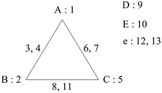
Linear graph of experiment.

Experimental results and ANOVA

ANOVA was used to discern the significance to the characteristic value of each selected parameter. The total sum of squared deviations (S_T) can be decomposed into two components: the sum of squared deviations due to each parameter (S_i) and the sum of the squared errors (S_ε). The percent contribution (ρ) is the percentage each parameter deviation contributes to the total sum (S_T). The F value, which is the ratio of the sum of squared deviation for each parameter (S_i) to the sum of squared errors (S_ε), is used to indicate quantitatively the significance of each parameter compared to the error terms. From the ANOVA results, a parameter with very low F and ρ values, which implies insignificance of the characteristic value, can be regarded as an error term along with other factors, such as economical efficiency and workability.

Table 3 shows the ANOVA results for R_a based on the experimental results summarized in Table 2, which shows that factors C and D and the interaction effects $A \times C$ and $B \times C$ are statistically meaningful, above the significance level of 10%. Table 4 shows the new ANOVA table after pooling insignificant terms into the error term. Figure 7 summarizes the influences of the various factors on the surface roughness R_a. Figure 7 illustrates the distributions and means of levels for each factor against the total mean of the data (dotted line).

Table 3.

Analysis of variance results for R_a.

Factor (i: parameter)	Sum of square, S_i	Degree. of freedom, φ	Mean square, V = S_i/φ	F = S_i/S_ε
A	105.29	2	52.68	1.7
B	66.1	2	33.05	1.07
C	1293.11	2	646.55	20.93*
D	246.64	2	123.32	3.99*
E	74.03	2	37.02	1.2
$A \times B$	28.76	4	7.19	0.23
$A \times C$	318.46	4	79.62	2.58*
$B \times C$	437.37	4	109.34	3.54*
Error	123.56	4	30.89
Total	2693.33	26

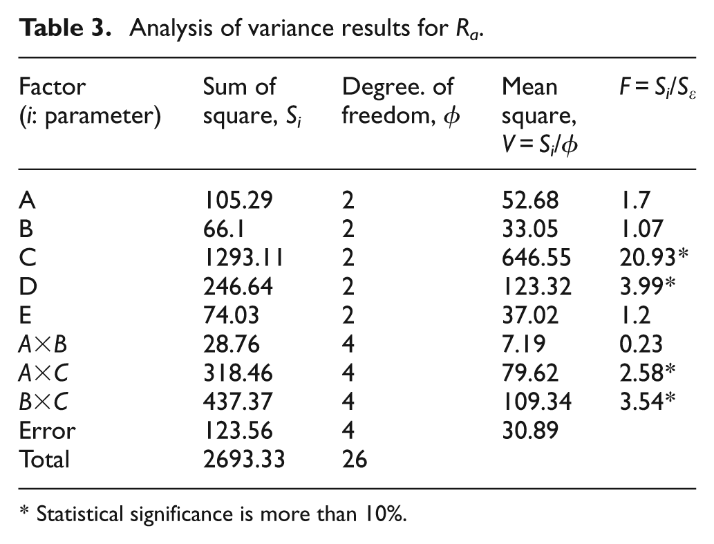
Statistical significance is more than 10%.

Table 4.

Analysis of variance results for R_a after pooling.

Factor	S_i	$ϕ$	V	F	ρ = (S_i/S_T × 100) (%)
A	105.29	2	52.68	2.33	3.93
B	66.1	2	33.05	1.46	2.45
C	1293.11	2	646.55	28.56*	48
D	246.64	2	123.32	5.45*	9.15
$A \times C$	318.46	4	79.62	3.52*	11.8
$B \times C$	437.37	4	109.34	4.83*	16.2
Error	226.36	10	22.64		8.4
Total	2693.33	26

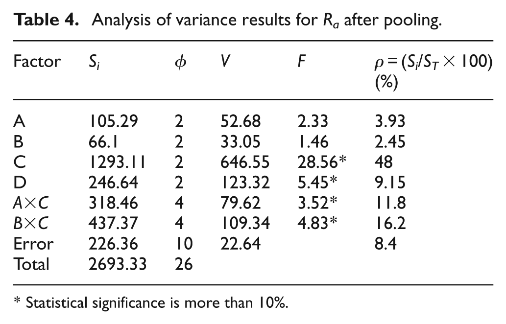
Statistical significance is more than 10%.

Figure 7.

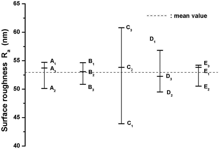
Influence of the factors to the surface roughness response R_a.

Similarly, ANOVA tables and the influence graph for R_max are shown in Tables 5 and 6 and Figure 8, respectively. Interaction effects are not considered in Table 6 because they are statistically insignificant. Factors C (gap size) and D (RPM) were selected as the most influential parameters to the surface roughness after polishing from the above results.

Table 5.

Analysis of variance results for R_max.

Factor	S_i	$ϕ$	V	F
A	21,092	2	10,546	9.43
B	6929	2	3465	3.10
C	153,694	2	76,847	68.73*
D	32,120	2	16,060	14.36*
E	43,130	2	2155	1.93
$A \times B$	12,434	4	3109	2.78
$A \times C$	27,331	4	6833	6.11
$B \times C$	13,819	4	3455	3.09
Error	4473	4	1118
Total	276,202	26

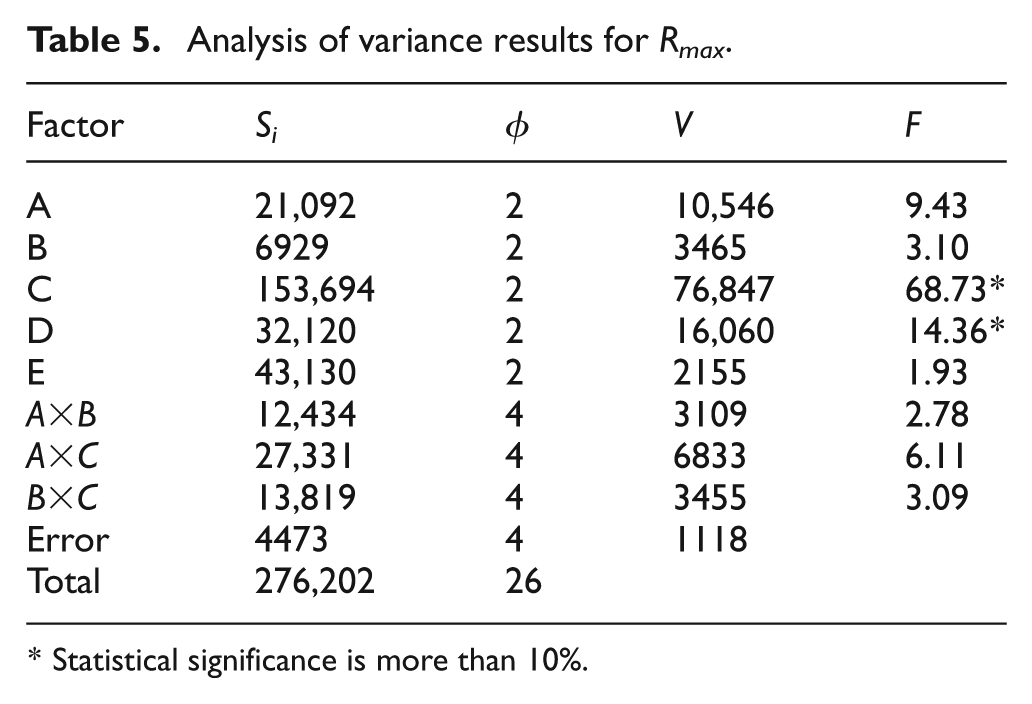
Statistical significance is more than 10%.

Table 6.

Analysis of variance results for R_max after pooling.

Factor	S_i	$ϕ$	V	F	$ρ (%)$
A	21,092	2	10,546	3.04	7.63
C	153,694	2	76,847	22.18*	55.64*
D	32,120	2	16,060	4.64*	11.62*
Error	69,296	20	3465		25
Total	276,202	26

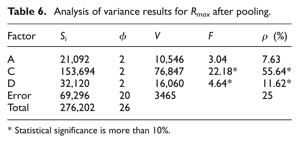
Statistical significance is more than 10%.

Figure 8.

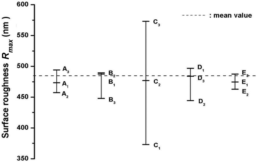
Influence of the factors to the surface roughness response R_max.

Process control

RtR control

There are many challenges to the application of polishing processes, such as MAF, in finishing, not the least of which is that it is a tedious, time-consuming task. The stable process control of MAF is challenging due to the unstable process conditions, including the inconsistency of the abrasive particles/slurry, variations in quill and sample surface conditions, and the lack of in-process monitoring sensors. If the process needs many runs with nanolevel target surface roughness value, a special process control scheme is needed.

A process control method known as RtR control, which has thus far been used mostly in the modern semiconductor industry,^19–21 is introduced to effectively implement MAF in precision mold finishing. RtR control is a form of discrete-time process control in which a particular equipment process recipe is modified between equipment runs to compensate for process drift, large shifts, and other disturbances to keep the outputs at the prescribed target values.¹⁹ This control scheme is most often used when information is difficult to acquire during the process, as in polishing. As in literature,^22,23 RtR control has been successfully applied to precision polishing processes such as CMP.

The target surface roughness values for the polishing process control were set to below 10 and 50 nm for R_a and R_max, respectively, because of the surface quality requirements for precision lens molds. Along with RPM and gap size, which were identified through DOE and ANOVA in the previous section, polishing time was also selected as a control factor. Because quantitative analysis of the physical processes going on in the polishing area (between the workpiece and the quill) is very complicated, the ranges for the process variables were determined experimentally. The selected control factors and their ranges are summarized in Table 7. Each control factor was shown to be nearly linear by linear regression analyses in the selected ranges. The results (response surfaces) are shown in Figure 9.

Table 7.

Selected control factors and ranges.

Factor	Lower bound	Upper bound
Gap (mm)	0.2	1
RPM (r/min)	250	1500
Polishing time (s)	120	480

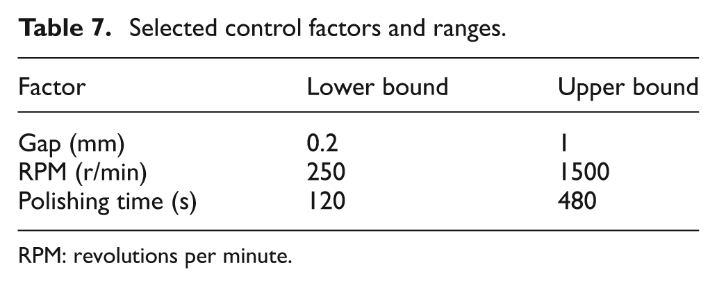
RPM: revolutions per minute.

Figure 9.

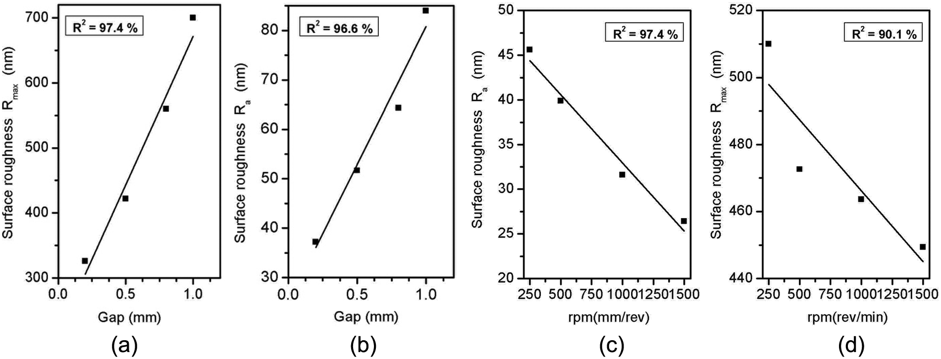
Response surfaces for R_a and R_max (with respect to gap size and RPM). (a) R_a vs. Gap size; (b) R_max vs. Gap size; (c) R_a vs. RPM; (d) R_max vs. RPM.

Each linearized polynomial regression model near the operating point can therefore be expressed as a multivariate model for the RtR controller.

y = A x + C

(2)

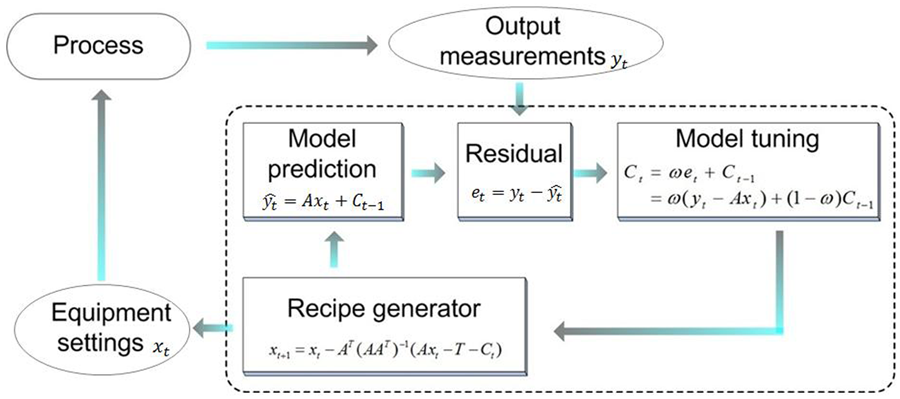
where y is the output vector (R_a and R_max) from the measurement after each process run, x is the input recipe vector (gap size, RPM, and polishing time), A is a matrix of model coefficients based on the preliminary experimental data, and C is a vector of offset drift terms. In this controller, we only adapt or update the offset terms while keeping the gain coefficients of A fixed. Figure 10 shows the structure of the RtR controller.²⁰

Figure 10.

Structure of the run-to-run controller with exponential weighted moving average (EWMA).

Model update

The measuring data taken at the end of each run were used as the output vectors in the RtR control process. The updating process was then executed based on the differences between the forecasted model and the output values. The exponential weighted moving average (EWMA) constant $ω$ is commonly used to update control models.²¹

C_{t} = ω (y_{t} - A x_{t}) + (1 - ω) C_{t -} 1 (ω \leq 1)

(3)

where $C_{t - 1}$ is the offset of previous process.

Because the model parameters are fixed, only offset drift values can be improved. The selection of the EWMA exponent $ω$ , which is determined by the past and present output values, has a large influence on the updated outputs. If the value of $ω$ is close to 1, it gives more weight to recent values and shows a better response to noise; however, if the noise in the process is large, the output value can fluctuate too much. Conversely, if it is close to 0, giving more weight to previous values, the response to noise is minimal. Care should therefore be taken when selecting the $ω$ value. An optimal control theory is applied to generate the control factor values according to the offset drift updates.

{min {‖ x_{t} - x_{t - 1} ‖}^{2} |}_{Ax = b}

L = \frac{1}{2} (x_{t} - x_{t - 1})^{T} (x_{t} - x_{t - 1}) + λ^{T} (A x_{t} - b), b = (T - C_{t - 1})

(4)

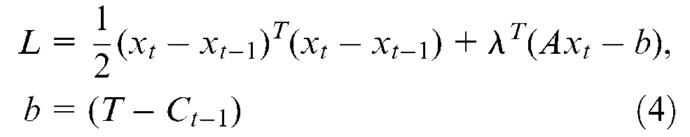
where x_t₋₁ is the recipe from previous run, A is the parameter drift, λ is the Lagrange multiplier, L is the equation to minimize, T is the desired output, and b is the difference between target and offset of previous process.

By differentiating with respect to $x$ , equation (4) becomes

x_{t} - x_{t - 1} = - A^{T} λ

(5)

By multiplying both sides by A and rearranging in terms of $λ$ , we get

A x_{t} = A x_{t - 1} - A A^{T} λ = b, λ = {(A A^{T})}^{-}^{1} (A x_{t - 1} - b)

(6)

Then, the final form with respect to x is

x_{t} = x_{t - 1} - A^{T} {(A A^{T})}^{-}^{1} (A x_{t - 1} - b)

(7)

The values of the control factor can be acquired using the optimal control condition for each process based on equation (7).

Process control and results

Because surface roughness output values can be nearly linearized within the design parameter ranges (Figure 9), RtR process control with EWMA was exercised for the polishing process. The initial values of equation (2), measured from experiments are shown as follows

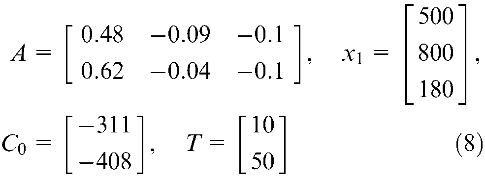
A = [\begin{matrix} \begin{matrix} 0.48 & - 0.09 & - 0.1 \end{matrix} \\ \begin{matrix} 0.62 & - 0.04 & - 0.1 \end{matrix} \end{matrix}], x_{1} = [\begin{matrix} 500 \\ 800 \\ 180 \end{matrix}], C_{0} = [\begin{matrix} - 311 \\ - 408 \end{matrix}], T = [\begin{matrix} 10 \\ 50 \end{matrix}]

(8)

where output vector y = [R_a (nm) R_max (nm)]^T and input vector x = [gap (µm) RPM polishing time (s)]^T, as explained in the previous section. The fixed parameter drift (A) was determined using DOE, and the other values were decided based on preliminary experimental data.

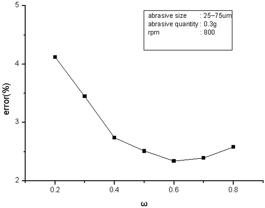
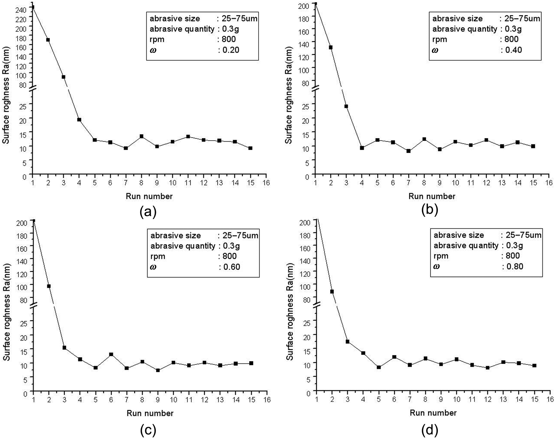
Before the main process control experiments, preliminary experiments were performed to determine the EWMA constant (ω). The experimental results in Figure 11 (with varying ω) show that R_a and R_max converge rapidly under the optimum $ω$ value of 0.6 (see smallest error, Figures 12 and 13). For this reason, an $ω$ value of 0.6 was selected for all subsequent polishing experiments.

Figure 11.

Process control output (R_a) with varying EWMA constant (ω).

Figure 12.

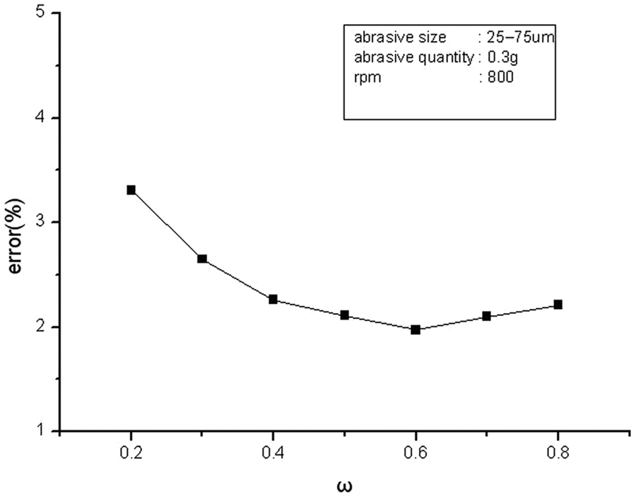
R_a errors with varying ω values.

Figure 13.

R_max errors with varying ω values.

The control model is updated using the output value measured at the end of each process run experiment in equation (3), and the input values of the control factors for the next run are generated by equation (4). Figure 14 shows the variations in input values during the experiments, and the subsequent output value (process) variation according to the updating are shown in Figure 15. As shown in Figure 15, the surface roughness values are kept below both target values after as little as three runs. Figure 16 compares typical polishing results after run 1 with those following run 15.

Figure 14.

Variation of control inputs during the process control: (a) gap, (b) RPM, and (c) time.

Figure 15.

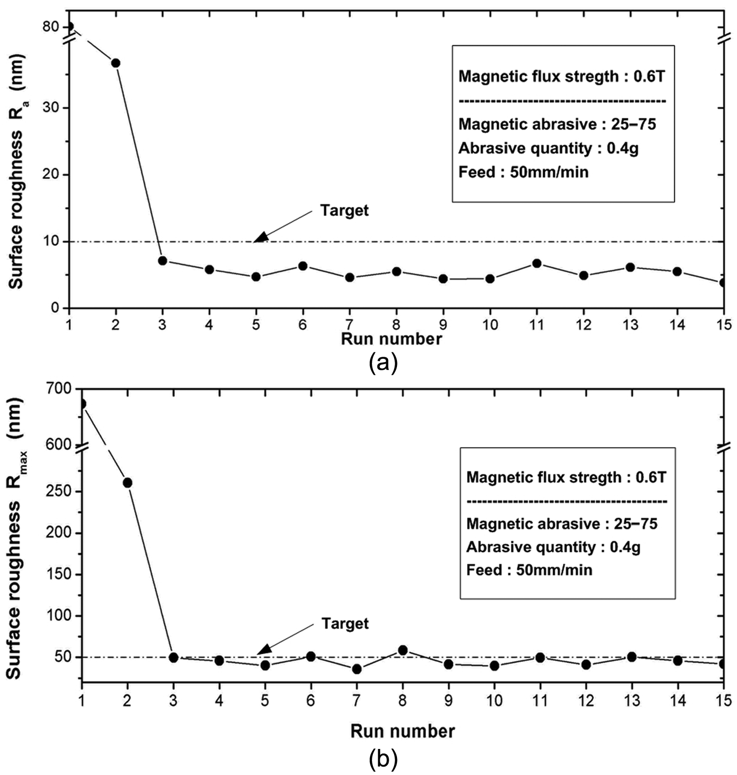
Variation in run-to-run control output: (a) R_a and (b) R_max.

Figure 16.

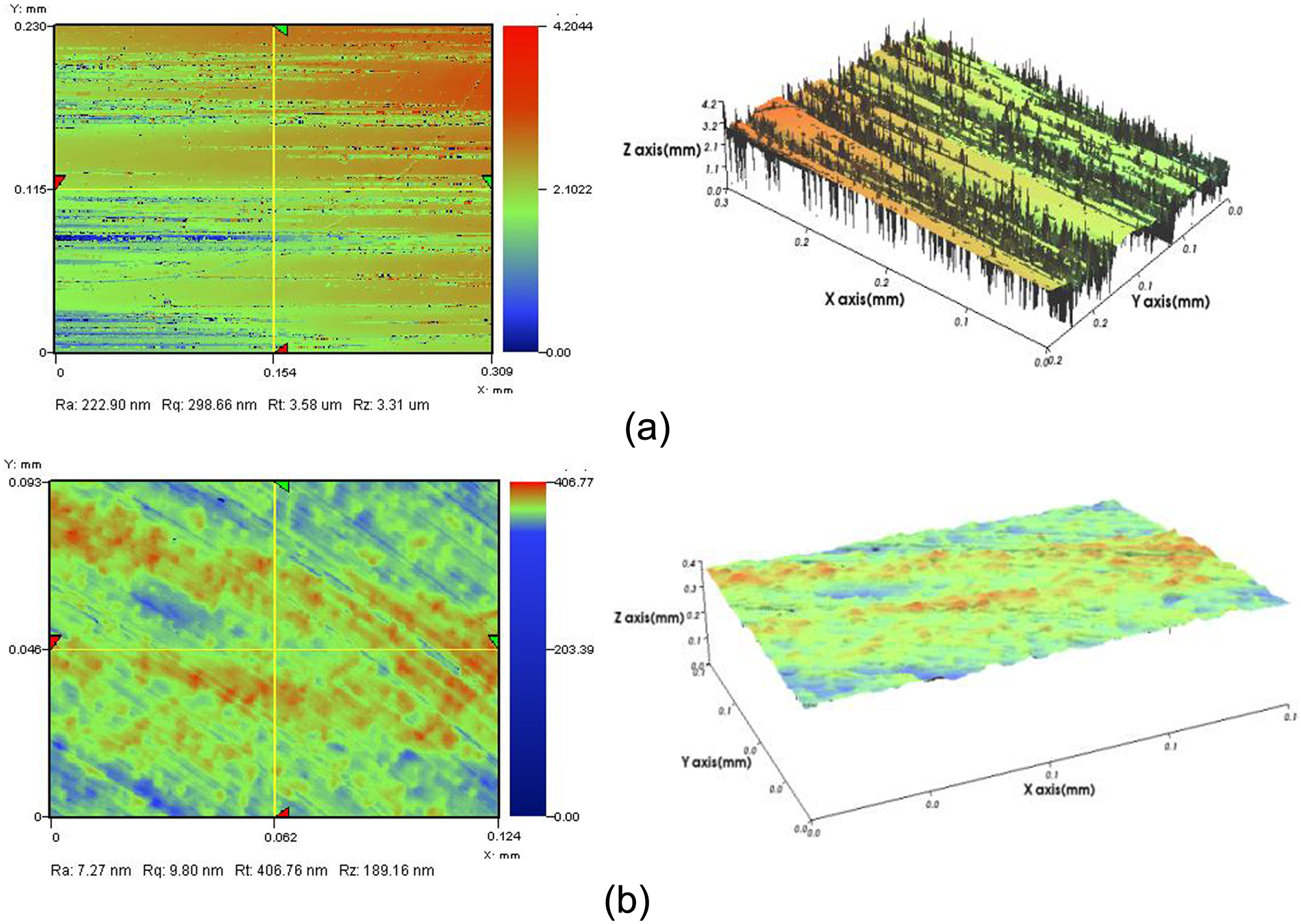
Typical measurement results of surface roughness: (a) run number 1 (R_a = 222.90 nm) and (b) run number 15 (R_a = 7.27 nm).

Conclusion

MAF, a polishing process using specially manufactured bonded magnetic abrasive particles, was applied to precision lens mold polishing. Polishing experiments were performed using the RtR control method to generate and maintain the nanometer-level surface roughness of the STAVAX S136 workpiece materials.

The conclusions are as follows:

Through analysis, including DOE and ANOVA, the most influential polishing control parameters, gap size, RPM, and polishing time were selected and the suitability of RtR control for the polishing process was validated.

Under RtR control with the selected parameters, surface roughness values were successfully maintained below the target values (10 and 50 nm for R_a and R_max, respectively), regardless of external factors, such as the wear on the abrasive particles, irregular surface characteristics of the workpiece, and the changes in polishing conditions.

With the applied control scheme and polishing setup, MAF is shown to be readily adaptable and viable for automated ultraprecision polishing applications such as lens mold polishing.

Footnotes

Funding

This work was supported by the research fund of College of Engineering at Hanyang University (HY-2011-N).

References

Zhang

Kuriyagawa

Kaka

. Investigation into electrorheological fluid-assisted polishing. Int J Mach Tool Manu 2005; 45: 1461–1467.

Kuriyagawa

Saeki

Syoji

. Electrorheological fluid-assisted ultra-precision polishing for small three-dimensional parts. J Soc Precis Eng Nanotechnol 2002; 26: 370–380.

Larson

. The structure and rheology of complex fluids. New York: Oxford University Press, 1999, pp.219–220.

Kordonski

Golini

. Progress update in magnetorheological finishing. Int J Mod Phys B 1999; 13: 205–212.

Cheng

Yeung

Tong

. Viscosity behavior of magnetic suspensions in fluid-assisted finishing. Nat Sci 2008; 18: 91–96.

Lin

Yang

Chow

. Study of magnetic abrasive finishing in free-form surface operations using the Taguchi method. Int J Adv Manuf Tech 2007; 34: 122–130.

Yamaguchi

Shinmura

. Study of the surface modification resulting from an internal magnetic abrasive finishing process. Wear 2001; 225–229: 246–255.

Jain

Kumar

Behera

. Effect of working gap and circumferential speed on the performance of magnetic abrasive finishing process. Wear 2001; 250: 384–390.

Jayswal

Jain

Dixit

. Modeling and simulation of magnetic abrasive finishing process. Int J Adv Manuf Tech 2005; 26: 477–490.

10.

Chang

Yan

Hsu

. Study in cylindrical magnetic abrasive finishing using unbonded magnetic abrasives. Int J Mach Tool Manu 2002; 42: 575–583.

11.

Yin

Shinmura

. A comparative study: polishing characteristics and its mechanisms of three vibration modes in vibration-assisted magnetic abrasive polishing. Int J Mach Tool Manu 2004; 44: 383–390.

12.

Park

Ahn

Lee

. Nano-scale precision polishing characteristics using a micro quill and magnetic chain structure. J Korean Soc Precis Eng 2004; 21(8): 34–42.

13.

Park

Ahn

Yoon

. Development of ultraprecision finishing technique using bonded magnetic abrasives. J KSMTE 2003; 12(1): 59–66.

14.

Lee

. Prediction of surface roughness in magnetic abrasive finishing using acoustic emission and force sensor data fusion. Proc IMechE, Part B: J Engineering Manufacture 2011; 225: 853–865.

15.

Feign

Kremen

. Magnetic abrasive powder and method of producing the same. Patent 5846270, USA, 1998.

16.

Ahn

Park

Min

. Method for manufacturing magnetic abrasive particle by mechanical alloying. Patent 100456234, Korea, 2004.

17.

Preston

. The theory and design of plate glass polishing machine. J Soc Glass Technol 1927; 11: 214–256.

18.

Taguchi

Yokoyama

. Taguchi methods-design of experiments. Dearborn, MI: ASI Press, 1993.

19.

Zhang

Deun

Baras

. Run to run control methods based on the DHOBE algorithm. Automatica 2003; 39: 35–45.

20.

Sachs

Ingolfsson

. Run by run process control: combining SPC and feedback control. IEEE T Semiconduct M 1995; 8: 26–43.

21.

Moyne

Castillo

Hurwitz

. Run-to-run control in semiconductor manufacturing. Boca Raton, FL: CRC Press, 2001.

22.

Boning

Moyne

Smith

. Run by run control of CMP. IEEE Trans Compon Packag Manuf Tech C 1996; 19(4): 307–313.

23.

Wang

. Developing a neural network-based run-to run process controller for chemical-mechanical planarization. Int J Adv Manuf Tech 2006; 28: 899–908.

Run-to-run process control of magnetic abrasive finishing using bonded abrasive particles

Abstract

Keywords

Introduction

MAP process

Magnetic abrasives

Polishing mechanism

Experimental setup

Process analysis using DOE

DOE

Experimental results and ANOVA

Process control

RtR control

Model update

Process control and results

Conclusion

Footnotes

Funding

References