
Abstract
Three methods of simulation of two-process profiles were compared. An idea for the best method is to impose a random Gaussian profile on the valley profile. A special procedure was developed by the present authors to obtain desired values of skewness and correlation length. The extension of this method was used in order to model three-dimensional surface topography after two processes. The imposition method was used for plateau-honed cylinder surface topographies simulation. The mating accuracy of modelled and measured topographies was good, taking into account the complicated character of plateau-honed cylinder surfaces.
Introduction
Cylinder, piston skirt, piston rings, valve train, crankshaft and its bearings are the major lubricated components in a reciprocating engine. The surface finish of cylinder bores is one of the most substantial factors influencing the friction, wear and lubrication of co-acting surfaces within the engine. Cylinder surface topography affects running-in duration, oil consumption, exhaust gases emission and engine performance.1–7 Cylinder liner machining is difficult because the demands on good sealing and optimal lubrication are antagonistic. The plateau-honing process is commonly applied to produce a specific cylinder surface. The final topography is a result of the two last steps in the plateau-honing process: coarse honing and plateau honing. A plateau-honed cylinder surface ensures, simultaneously, a good sliding property of a smooth surface and a great ability to retain oil on a porous surface. Plateaued surfaces have been machined to simulate those that result from normal running-in. These surfaces are said to have advantages over conventional surfaces.1–4,8,9
The functional behaviour of surfaces can be predicted numerically. Time and cost of experimental research can be reduced by surface roughness simulation. Usually, Gaussian random surfaces of assumed properties were modelled. Profiles were generated using time series models.10–12 Sasajimi and Tsukada, 13 and Ganti and Bhushan 14 modelled fractal rough profiles of symmetric ordinate distribution.
Simulation of areal (three-dimensional (3D)) surfaces became popular. Patir 15 used the linear transformation of a matrix in order to produce a rough surface having a specified autocorrelation function. A major disadvantage of Patir’s method was that it required the solution of a non-linear system of equations, which is both storage space and time limiting. The procedure developed by Bakolas 16 extended Patir’s method, employing the non-linear conjugate gradient method (NCGM) and fast Fourier transform (FFT) in order to get convergence and minimize the storage requirement. Oriented rough surfaces can be generated by this method. Time series and FFTs are popular in generating 3D surfaces. Time series models were used by Whitehouse 17 , Gu and Huang, 18 Hong and Ehmann, 19 Uchidate et al., 20 Nemoto et al., 21 and Uchidate et al. 22
Usually, after application of time series models, only a few points near the origin of the autocorrelation function can be properly simulated. In order to cope with the storage space and time limitations of the mentioned methods a FFT application was proposed. Hu and Tonder, 23 Newland 24 and Wu 25 recommended similar models that can be used for the generation of rough surfaces of Gaussian ordinate distribution. Wu 25 found that his and Newland’s models were superior to Hu and Tonder’s method, however Wu’s method was the best one (this was confirmed in another investigation 26 ). For a very small correlation length, all three methods are acceptable. NCGM 16 was compared with the FFT method generated by Hu and Tonder. 23 The results showed that both methods can correctly produce rough surfaces with small correlation lengths, for higher correlation lengths the NCGM method gave better results. 27
Non-Gaussian random surfaces, with given values of skewness and kurtosis, were mainly achieved using the Johnson translatory system. 28 Watson and Spedding, 29 Uchidate et al., 20 as well as Gu and Huang 18 used an autoregressive moving average (ARMA) method, Hu and Tonder 23 used an FFT method and Bakolas 16 used an NCGM method. A digital filter was employed by Hu and Tonder 23 to generate an output sequence of known autocorrelation function by a linear transformation system. For the generation of profiles of non-Gaussian ordinate distribution, the Gaussian input sequence was transformed to an output sequence with appropriate skewness and kurtosis using the Johnson translatory system of distribution. Seong and Peterka 30 used the FFT to generate a non-Gaussian pressure time series and so did Kumar and Stathopoulos. 31 Their models can be applied to simulation of non-Gaussian rough surfaces. The amplitude part was constructed by Wu 32 from an assumed spectral density function or autocorrelation function.
The other method of plateau-honed surface topography simulation relies on the fact that the fine surface created during the final machining process has its characteristic amplitude distribution and the whole system represents a transitional topography. The resulting topography is that of the original coarse honed surface up to some height. Above this height is superimposed another distribution, also Gaussian but smoother. This method is based on the superimposition of a random Gaussian surface on the base surface. 33
There were also scientific works devoted especially to simulation of cylinder surfaces of non-symmetric ordinate distribution. The analysis of this type of surfaces is a serious problem. Rosen et al. 34 attempted to select suitable surface roughness parameters in the context of current standard and industrial applications. However, roughness parameters can be distorted as the results of improper digital filtering. 35 Rosen and Crafford 36 and Rosen 37 generated a 3D synthetic surface on the basis of a few parameters. Jablonski used a fractal approach to generate a plateau-honed cylinder surface. 38 Voronov et al. 39 discusses the modelling of deep holes during honing. The dynamic model of honing, including the models of tool dynamics, cutting forces calculation and new surface formation, is presented. Feng et al. 40 applies artificial neural networks to develop an empirical model for the honing process of engine cylinder liners. In Feng et al., 41 a rigorous procedure was proposed for evaluating the validation and data splitting methods in predictive regression modelling. Experimental data from a honing surface roughness study was used to illustrate this methodology.
In this paper, three methods of simulation of a multi-process profile were compared. An extension of the best method was used in order to model 3D surface topography.
Simulation of 2D profiles
Procedures of calculation
Two methods, as proposed in Hu and Tonder 23 and Wu, 32 based on a FFT approach were analysed. Profiles of desired parameters characterizing the shape of the ordinate distribution, like skewness and kurtosis, as well as autocorrelation or power spectral density functions, can be modelled. There were the following input parameters: standard deviation of height Pq, skewness Psk, kurtosis Pku, as well as the correlation length CL (the distance, at which the autocorrelation function slowly decays to 0.1 value).
In the first method, a digital filter was employed by Hu and Tonder 23 to generate an output sequence of known autocorrelation function by a linear transformation system. For the generation of profiles of non-Gaussian ordinate distribution, the Gaussian input sequence was transformed to an output sequence with appropriate skewness and kurtosis using the Johnson translatory system of distributions. 28
In the second method, the amplitude part was constructed by Wu 32 from a given spectral density function. The Johnson translatory system was used to obtain the phase part. By iteration and adjusting the input skewness and kurtosis, the required non-Gaussian surfaces can be generated.
In the third approach, the imposition method was used based on previous research. 33 One can obtain the parameters characterizing two-process surfaces from the material ratio curve probability plot. In this graph, two straight lines are visible and their slopes give the height standard deviations for the corresponding processes. The abscissa Pmq of the intersection point of the two straight lines on the normal probability graph defines the separation of plateau and base textures (see Figure 1). The plateau roughness Ppq, valley roughness Pvq and Pmq are three parameters characterizing a plateau-honed surface (ISO 13565-3 standard). 42 The plateau depth Pd is also shown in Figure 2. Ppq, Pvq, Pmq and Pd parameters are connected by the following formula 43
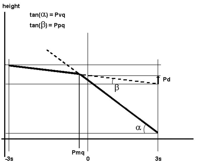
Parameters described in ISO 13565-3 standard. 42
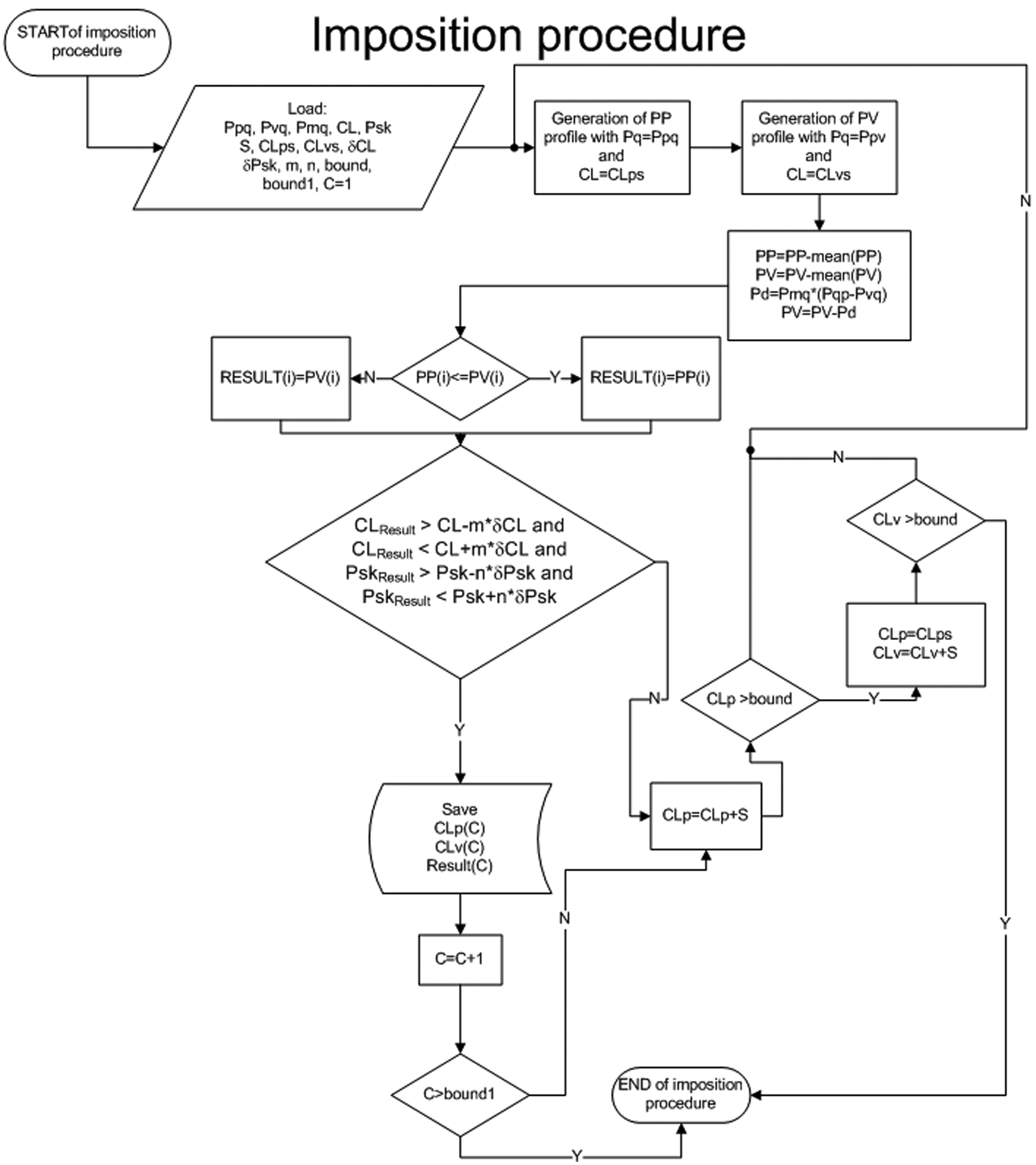
Procedure of 2D profile modelling using the imposition method (IM).

Two-process profiles can be simulated by generation of two profiles of the Gaussian ordinate distribution: plateau (PP) and valley (PV). Distances between their mean lines Pd should be assumed. Then points of smaller ordinates from these two profiles ought to be selected.
On the basis of previous research, 26 the present authors used FFT to generate Gaussian profiles according to Wu. 25 Each Gaussian profile was completely characterized by two parameters: the standard deviation of height (Pqp for plateau profile and Pvq for valley profile) and the correlation length (CLp and CLv). Autocorrelation functions of computer-generated profiles had exponential shapes.
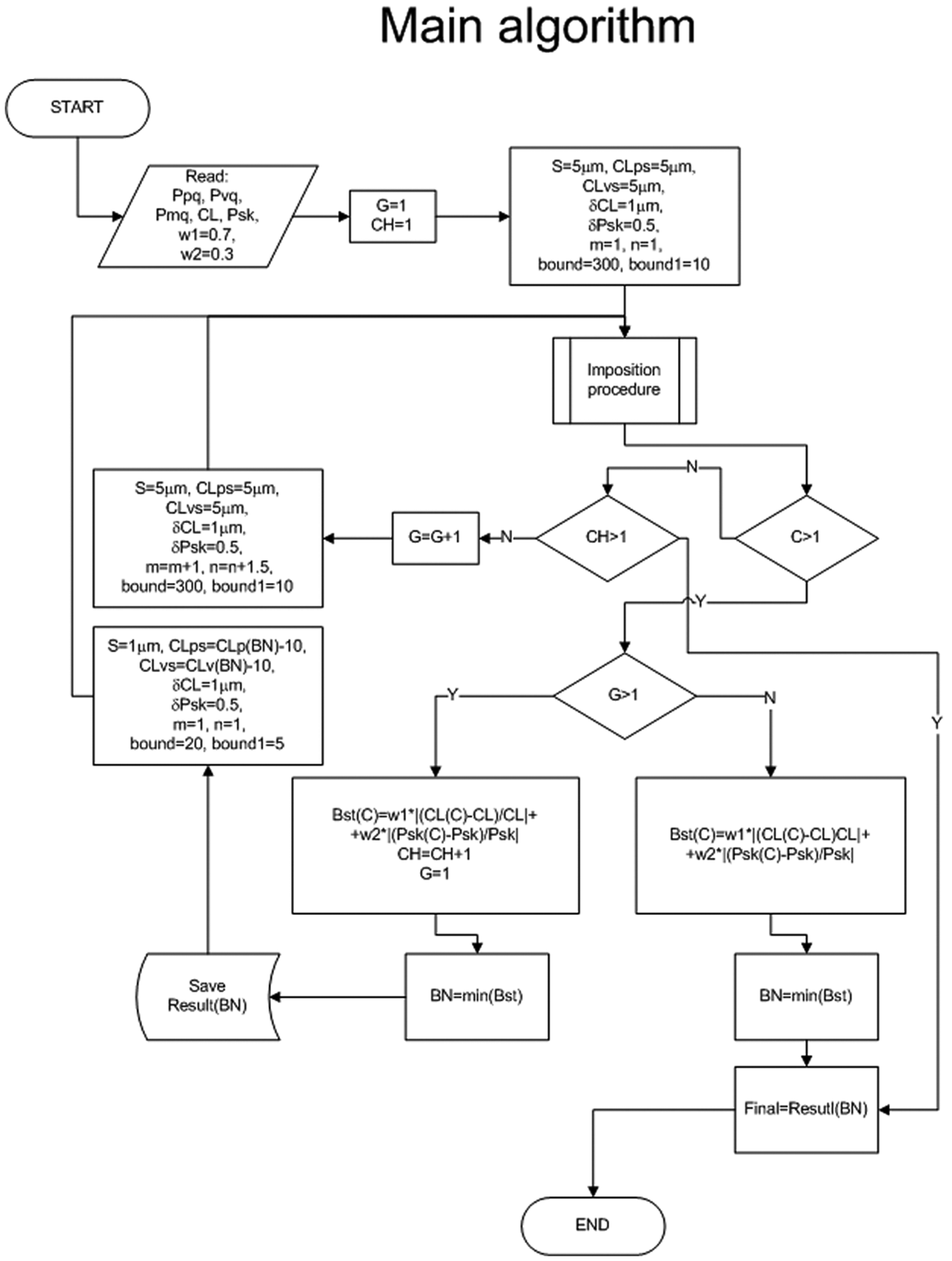
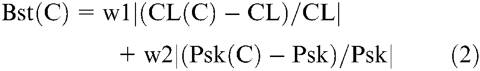
The original procedure was developed in order to obtain prescribed values of skewness Psk and correlation length CL of the modelled resultant profile (in addition to Pqp, Pqv and Pmq parameters). Therefore CL, Pqp, Pqv, Psk and Pmq were input values in this model. As the result of initial investigations, the tolerances of skewness and correlation length were set (δCL = 1 µm, δPsk = 0.5). Figures 2 and 3 present a flow chart of the modelling. Figure 2 shows the procedure of the main modelling, while Figure 3 presents the imposition procedure (part of the main modelling). Optimization was done automatically using a two-objectives optimization technique, differences between correlation length and skewness of modelled and measured profiles were minimized. The higher weight was attributed to correlation length CL difference (w1 = 0.7) than to skewness Psk deviation (w2 = 0.3). The weight attributed to correlation length was higher because functional importance of CL is bigger than that of Psk. Furthermore, skewness is sensitive to extreme ordinate values, therefore, an individual peak presence can affect the Psk parameter significantly, although such a peak may have no relevance to surface usefulness. First, profiles of a Gaussian ordinate distribution: PP with standard deviation of ordinates Pq equal to the Pqp parameter and PV of Pq equal to the Pqv parameter were generated with initial correlation lengths CLps and CLvs, respectively. Then these Gaussian profiles were superimposed for a plateau depth obtained from equation (1). This profile was stored when the correlation length and skewness of the resultant profile were within tolerance limits: CL ± δCL and PSk ± δPsk, respectively. Next, for the same PV profile, correlation length of the PP profile increased by a constant step S and the imposition procedure was repeated. In calculation, minimum and maximum values of correlation length were set to 5 µm and 300 µm, but the step S was 5 µm. When the correlation length of the PP profile reached maximum value (bound in Figures 2 and 3) the correlation length of the PV profile increased by a constant step, and this PV profile and the PP profiles with increasing correlation length by step S were superimposed. In calculation, the same minimum and maximum values of correlation lengths and steps S of PP and PV profiles were set. The calculation was interrupted when the number of stored profiles (C in Figures 2 and 3), with correlation length and skewness within tolerance limits, was higher than bound1. If not, all the PP and PV profiles with correlation lengths from the range: 5–300 µm were superimposed. The weighted relative difference Bst(C) between parameters CL and Psk of measured and modelled profiles was calculated using the following equation
Flow chart of 2D profile imposition procedure.
where CL(C) and Psk(C) are correlation lengths and the Psk parameter of modelled profile C.
When the number of stored profiles (C) was higher than 1, the profile BN of the smallest weighted difference Bst(C) was selected and stored. When only one profile for which CL and Psk parameters were within desired tolerances δCL and δPsk, respectively, or no such profiles were found (CH > 1 in Figure 2), the tolerances δCL and δPsk increased. The increase in δCL was smaller than the increase in δPsk. Then the imposition procedure was repeated. When in a new imposition process, only one profile or no profiles fulfilled conditions of the CL and Psk parameter values, tolerances of these parameters further increased and the imposition procedure was repeated again. Tolerances of the Psk parameter were nδPsk, of CL – mδCL; initially m = n = 1; in next iterations n = n + 1.5, m = m + 1. When more than one profile satisfied limiting conditions of the CL and Psk parameters, the best profile BN (of the smallest weighted difference) was selected and saved with correlation lengths CLp(BN) and CLs(BN). Next, tolerances of the CL and Psk parameters decreased to initial values. The imposition process was repeated again, for correlation lengths CLps and CLvs near CLp(BN) and CLs(BN) with the step S (1 µm) smaller than its initial value. It was found that this procedure, implemented in MATLAB, assured correct values of the analysed parameters.
This procedure can be shortened during plateau-honed profile modelling. It was found that for this type of profile correlation length of the plateau part CLp was not higher than correlation length of the valley part CLv. This should be taken into consideration in the imposition procedure. The described procedure can be used in order to model profiles, not only after plateau honing, but also after a low wear process (wear within the limits of original surface topography) of a profile of initially Gaussian ordinate distribution.
Results of 2D profile modelling
About 20 plateau-honed cylinder surfaces were analysed. Cylinders were honed by various methods and with tools of different design. Cylinder liners were classically plateau honed and slide honed. Cylinders were honed using SiC and diamond abrasives, and represent commercial manufacturing concepts.
The unfiltered levelled profile parameters were compared. Digital filtration was not used. Assessment length was 4 mm. A profile measurement gauge without skid was applied. The Hu and Tonder method 23 was called M1, the Wu method 32 was called M2, but the method of profiles imposition was called IM. Table 1 presents the average values of absolute relative errors of profile parameters values. These deviations were calculated in relation to parameters of measured profiles.
The average values of absolute relative deviations of modelled profiles parameters, %.
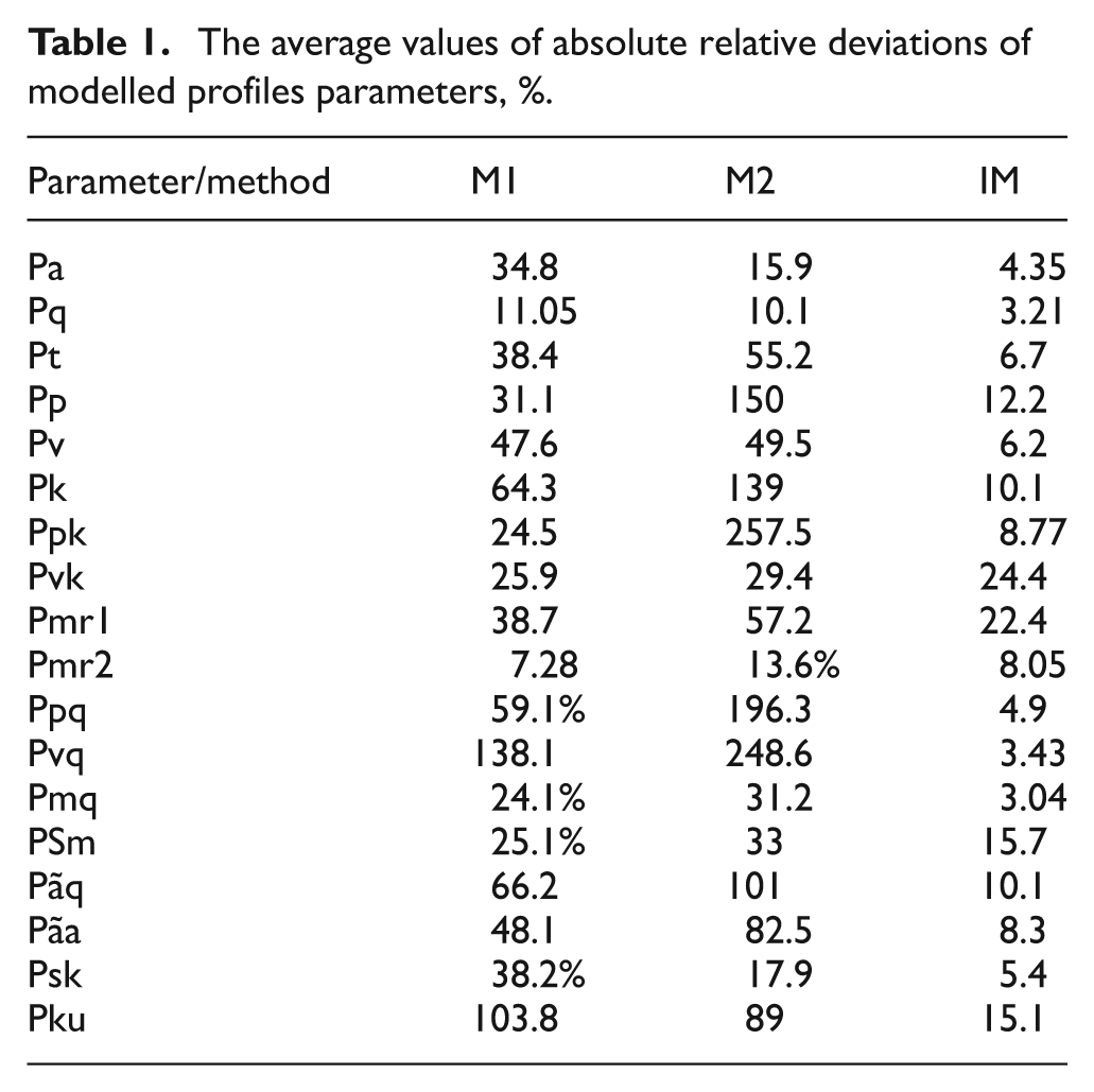
The following parameters were analysed: arithmetic mean height Pa, standard deviation of height Pq, maximum height Pt, maximum peak height Pp, maximum valley depth Pv, skewness Psk, mean peak spacing PSm, average profile slope PΔa and root mean squared (rms.) profile slope PΔq (most of these parameters are included in the ISO 4287 standard), 45 as well as functional parameters included in ISO 13565-2 44 (core depth Pk, reduced peak height Ppk, reduced valley depth Pvk, peak material ratio Pmr1 and valley material ratio Pmr2) and ISO 13565-3 42 (Ppq, Pvq and Pmq) standards.
The errors of the Pq parameter computation were lower than those of Pa. The small parameter distortion after using the IM method is interesting, because in this case Pq was not an input parameter, differently to other methods. The largest errors of the Pt parameter computation were obtained after using the M2 method, they were smaller after M1 and IM methods application. Deviations of statistical parameter computation were smaller than those of maximum amplitude parameters. The application of the IM method caused the smallest errors.
The errors of the Pp parameter computation were the highest after the M2 method, smaller after the M1 and the smallest after the IM method application. However deviations of the Pv parameter after M1 and M2 methods were similar, the absolute relative errors after the IM method application were the smallest. The distortions of the Rk family parameters were the largest after using the M2 method and the smallest after the IM procedure application.
Parameters included in the ISO 13565-3 42 standard were input parameters for the IM modelling method. Therefore, their average errors were smaller than 5% (maximum deviations were smaller than 10%). After the M2 method application, the errors were higher compared with the M1 method. Values of Ppq and Pvq parameters of modelled profiles were larger than those of measured profiles when the M1 and especially M2 methods were applied. When the M1 and M2 methods were applied, the values of the PSm parameter of modelled profiles were smaller than those of measured profiles. The smallest deviations were received after using the IM method.
Rms. slopes of modelled profiles PΔq were higher than those of measured profiles. The errors were the smallest after the IM method application. A similar tendency was found with regard to average slope PΔa, however, in this case the discrepancies were a little smaller. The small errors of computation of parameter characterizing the shape of the ordinate distribution Psk and Pku deserve attention because the Pku parameter was not an input parameter in this model.
In addition, the accuracy of the correlation length CL modelling was assessed. In 65% of the analysed cases the correlation lengths CL of modelled profiles were the closest to the values of the measured profiles after using the IM method; in other cases after the M2 method application. The IM method use causes a small underestimation, but M2 causes overestimation of the correlation length CL. When the M1 method was used, correlation length was overestimated, especially for its high assumed value. The average errors of CL determination were 10.99% after the IM method, 17.24% M2 and 74% the M1 method application.
Generally, the IM method was superior to M1 and M2 procedures with regard to model plateau-honed cylinder profiles. In the majority of cases, the errors of parameter computations were the smallest after using the IM method. Procedures M1 and M2 can generate the required non-Gaussian surfaces provided the skewness and kurtosis are not too large. The M2 method was better than the M1 model for profiles of higher correlation length. The errors of statistical parameter determinations were smaller than those of parameters describing maximum height. After the IM method application, the average errors of the following parameter determinations were larger than 10%: CL, Pp, Pk, Pvk, Pmr1, PSm, PΔq and Pku. Smaller errors of parameters Ppq, Pvq and Pmq determinations, in comparison with Pmr1, Ppk, Pvk, Pk and Pmr2 parameters, are the results of the fact that the first group of mentioned parameters were input values in the IM procedure. When this model was used, the mating accuracy was good, taking into account the complicated character of plateau-honed cylinder profiles.
Figures 4 and 5 present examples of measured and modelled profiles and their autocorrelation functions. The selected parameters values are also given.
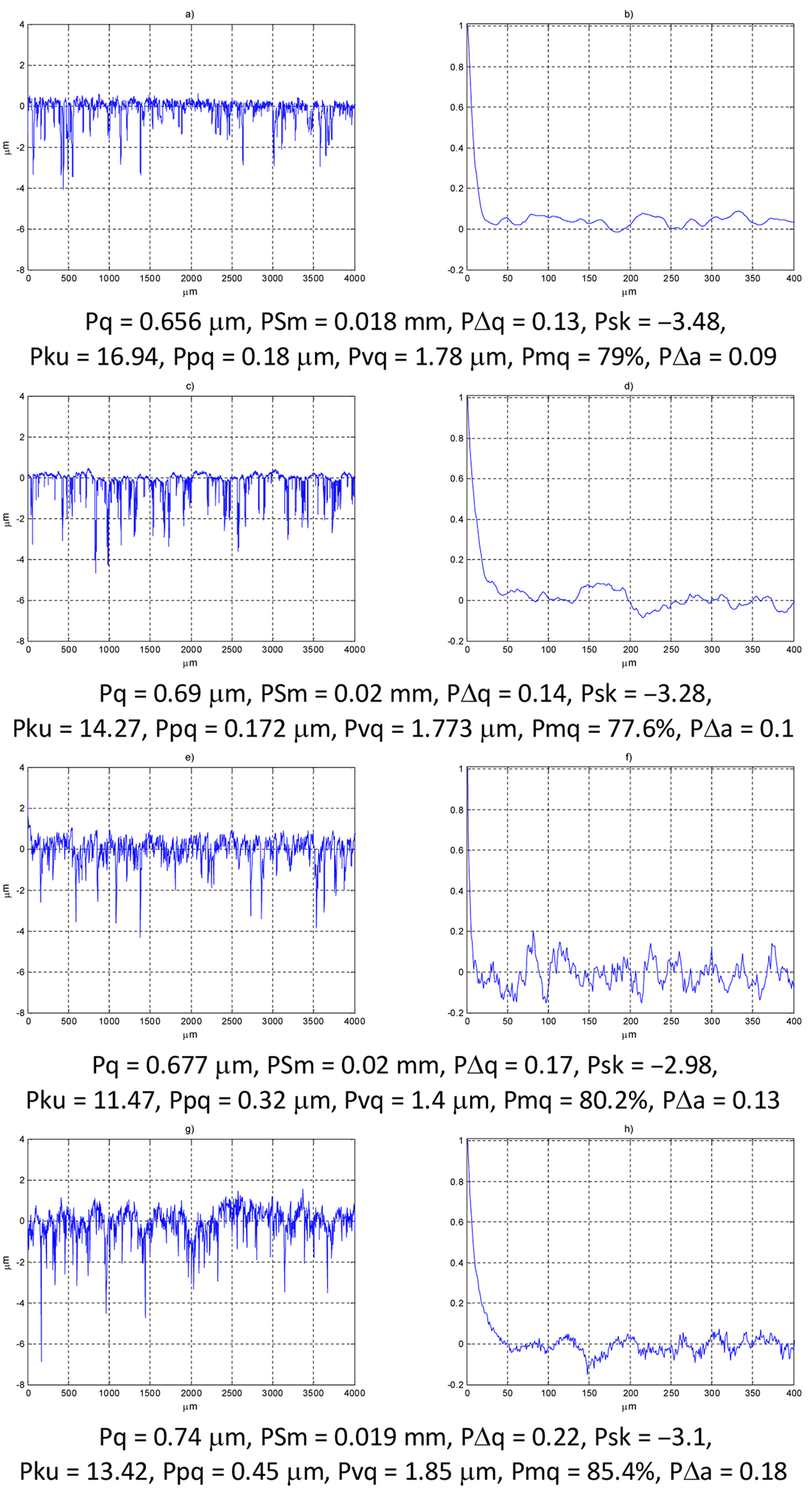
Measured profile (a); its autocorrelation function (b); profile modelled by the IM method (c); its autocorrelation function (d); profile modelled by the M1 method (e); its autocorrelation function (f); profile modelled by the M2 method (g); and its autocorrelation function (h).
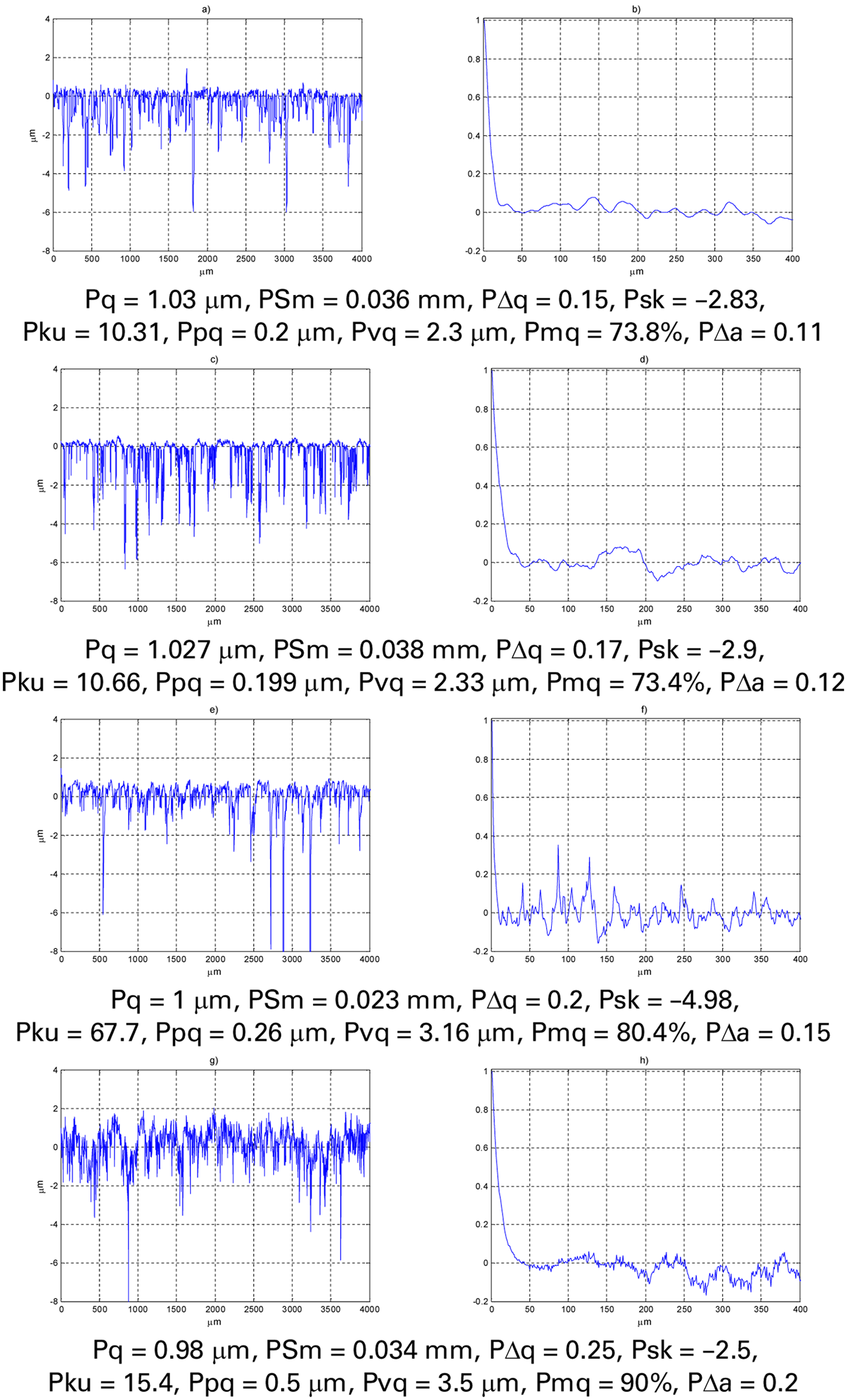
Measured profile (a); its autocorrelation function (b); profile modelled by the IM method (c); its autocorrelation function (d); profile modelled by the M1 method (e); its autocorrelation function (f); profile modelled by the M2 method (g); and its autocorrelation function (h).
Simulation of 3D surface topography of plateau honed cylinder liners
Simulation of one-process cylinder surface topography
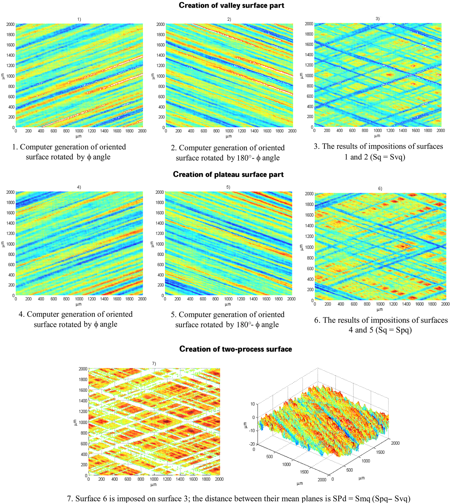
The IM method was extended into three dimensions. The one-process honed structure was simulated. A special procedure was used in order to obtain the honing angle α (see Figure 6) and parameters describing honed-cylinder surface topography. In the first stage, a one-directional (1D) surface oriented in the measurement direction was obtained. This surface was characterized by standard deviation of height Sq and correlation lengths in orthogonal directions CLx and CLy. Next, this surface was rotated by Φ angle equalled to half of the honing angle α using rotation of the coordinate system. This surface was stored. Next, the initial 1D surface was rotated by 180°–Φ angle. This surface was also stored. These two oriented surfaces were then superimposed, provided their reference planes were on the same level. For all the points of these surfaces the smaller ordinates were selected. It was found that the Sq parameter of the crossed surface topography was 1.2–1.25 times lower than that of the initial one-directional surface. Therefore the standard deviation of height of the initial 1D texture should be corrected (increased). This allowed the correct values of the Sq parameter of the modelled surface to be obtained. Parameters describing spatial properties ought to be also matched. It should be done by changes in correlation lengths of the initial 1D surface (before rotation) and selection of those values for which the difference between spatial parameters of modelled and measured surfaces would be the smallest. Average arithmetical slope SΔa depends only on spacing properties for the same surface topography height characterized by the Sq parameter. Evidence that the ratio of profile mean arithmetical slopes in orthogonal directions characterizes anisotropy of cylinder surfaces is substantial. A change in the SΔa parameter was achieved by changes in the correlation lengths of the 1D structure. For example, when the larger correlation length CLx of the initial structure (before rotation) was the same, the increase in correlation length in the perpendicular direction CLy caused an increase in correlation lengths in axial and circumferential directions (CLa and CLc, respectively) of the modelled cylinder surface, thus a decrease in surface slope. Since the average slope is proportional to height, the dependence between Φ angle and average slope SΔa of the crossed surface for various correlation lengths of the initial 1D surface can be helpful in initial estimation of CLx and CLy correlation lengths. Figure 7 presents an example of this dependence. The Sq parameter value was 1 µm, sampling intervals in perpendicular directions were 5 µm. However, one should check matching accuracy of modelled and measured surfaces, and if necessary, correct correlation lengths CLx and CLy. In modelling, more initial correlation lengths than presented in Figure 7 should be used.
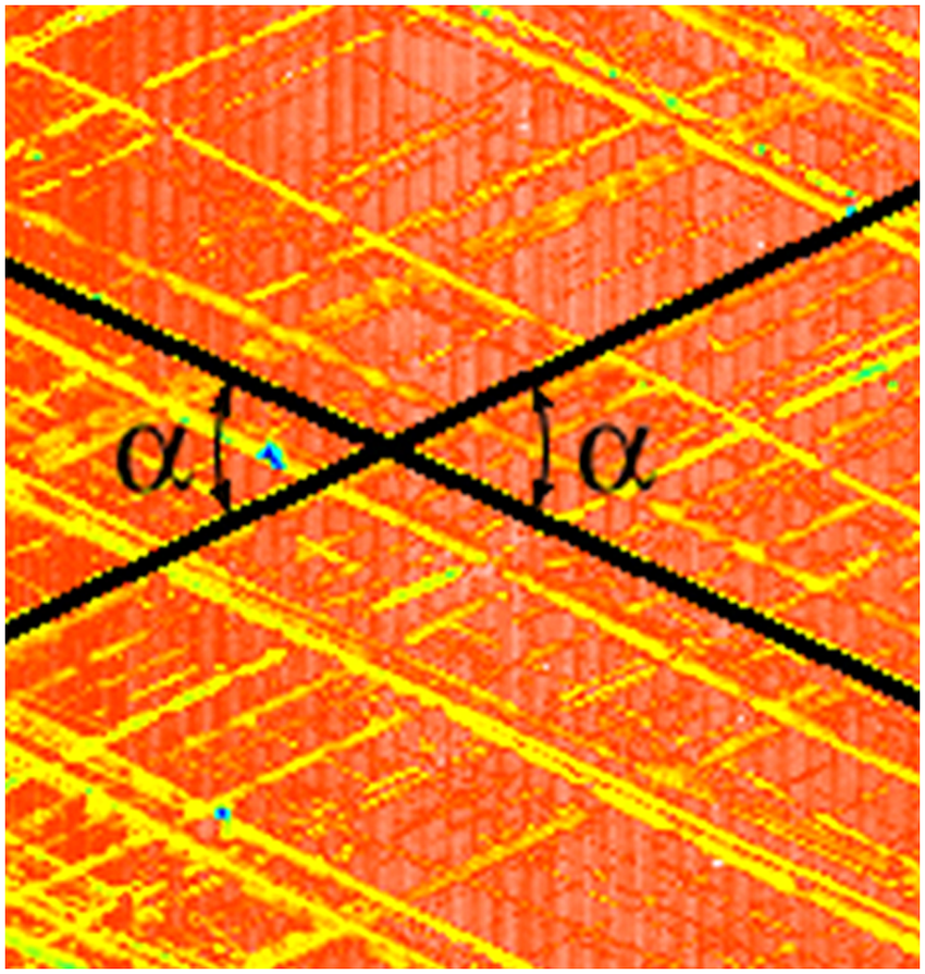
Cylinder texture with the honing angle α.
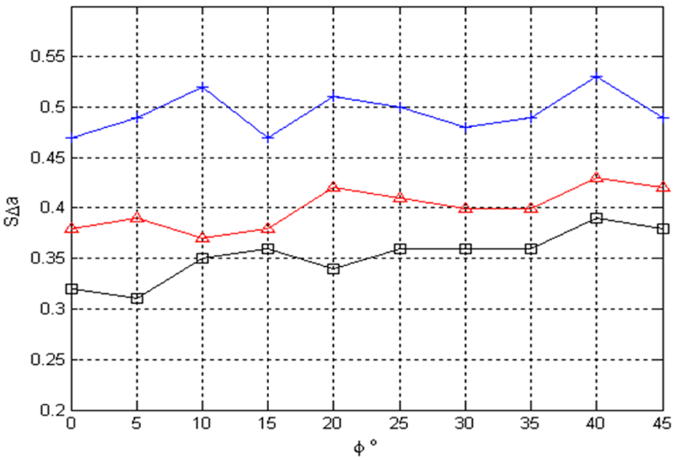
The effect of Φ angle on mean arithmetical slope SΔa of the crossed surface. Correlation lengths of the 1D surface (before rotation) are 5 and 400 µm (crosses), 20 and 400 µm (triangles), as well as 10 and 200 µm (squares).
Prediction of parameters of 3D surface topographies after two processes
In 3D surface topography modelling, only the imposition method IM was used. A similar procedure to the simulation of 2D profiles was applied. Two crossed surfaces of Gaussian ordinate distribution were superimposed. The procedure of modelling will be described later. However the procedure of 3D surface topography after two process simulations is time consuming. Therefore, the possibility of a decrease in the number of imposed surface topographies was taken into consideration. Prediction of parameters of stratified surfaces can be helpful.
Similarly to profiles, 33 parameter values of the resultant surface topography should be

where SR is a parameter of the resultant surface, Sp and Sv are parameters of the plateau and valley parts of the surface, respectively. The Smq parameter should be in linear scale. 40 simulated topographies after plateau honing were analysed. The values of Spq parameters of the resultant surfaces were in the range 0.23–0.52 µm, however, of Svq 0.47–1.73 µm. Correlation lengths of the valley surface (7–100 µm) were not smaller than those of the plateau surface (4–11 µm). This dependence was found after analysis of the measured plateau-honed cylinder surfaces. The values of the Smq parameter were in the range 50–94% (this range was also selected based on the analysis of the measured plateau-honed surfaces). For surface topographies of Gaussian ordinate distribution modelling, the method developed by Wu 25 was used.
It was found during simulation of two-process profiles 33 that the smallest errors were obtained for estimating profile slope. Therefore, the attempt was made to predict the average slope SΔa of the 3D surface. The slopes were calculated by two-point finite difference approximations. The surface slope in each point was calculated by taking the square root of squares of the two perpendicular slopes. Similarly to profile analysis, average slope SΔa errors were very low (mean errors were 3.5%, maximum errors were 11.6%). In calculations, the measured area comprised 512 × 512 points. When the number of measuring points is small and finite difference approximations for the slopes are used, greater errors can be made by averaging the slopes of the two underlying processes weighted with their fractional area contribution. Deviations of the parameters: rms. slope SΔq, arithmetical mean height Sa and rms. height Sq prediction, were a little higher; not smaller than 7%, on average. The presented comparatively small uncertainties were caused by the fact that correlation lengths of the valley surface part were not smaller than those of the plateau surface part. Errors of estimation of the other analysed parameters: maximum height Sz, ten point height S10z, arithmetic mean peak curvature Spc, autocorrelation lengths Sal, and texture aspect ratio Str (ISO 25178) 46 were larger. Accurate information of the parameter SΔa prediction can be helpful in 3D surface topography modelling.
Figure 8 presents examples of surfaces of Gaussian ordinate distribution (plateau and valley) and the resultant surface topography with selected parameters describing them.
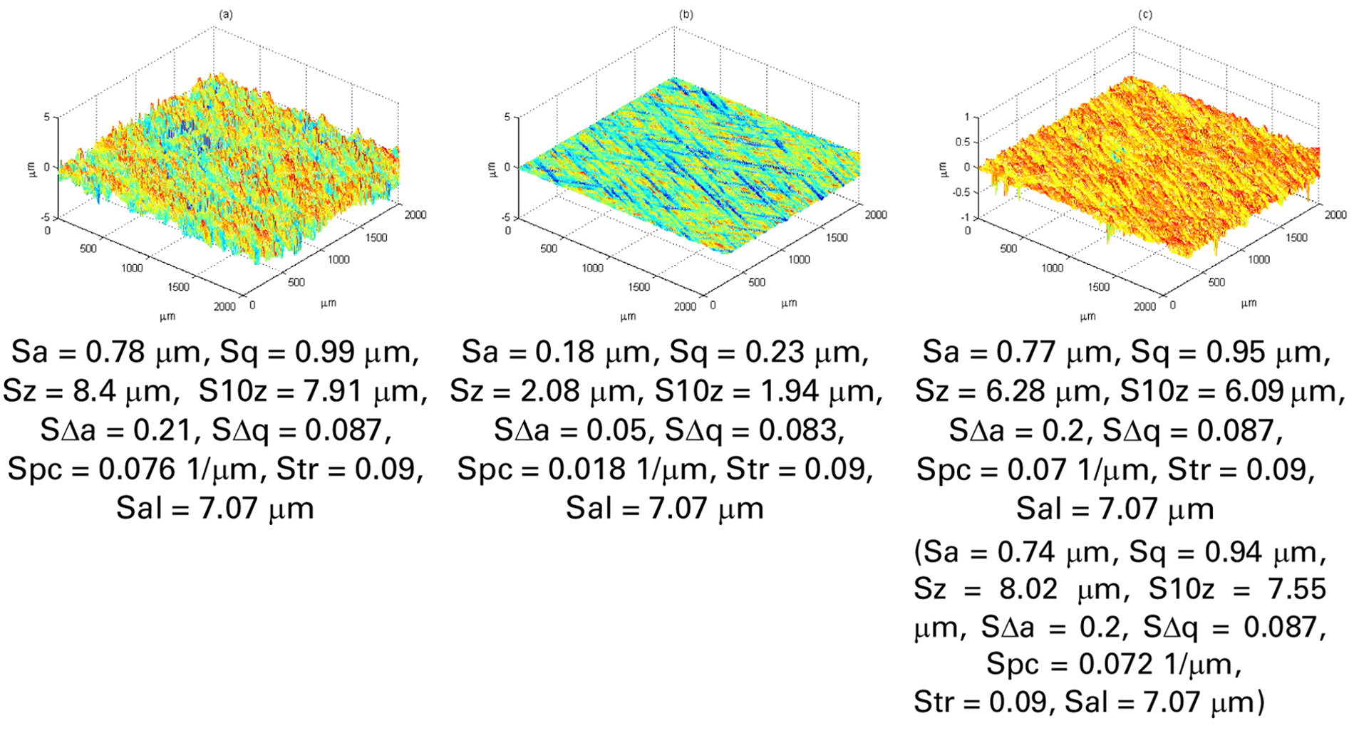
Surface topographies of normal ordinate distribution: valley (a) and plateau (b) and resulted (c) with selected parameters describing them (in brackets, parameters calculated from equation (3) are given for Spq = 0.23 µm, Svq = 0.99 µm and Smq = 93,7 %).
Modelling procedure
First, crossed structures of Gaussian ordinate distribution (of honing angle α equal to that of the measured surface) characterized by Sq parameter equal to Sqv and Sqp parameters of the plateau-honed surface were created (the procedure of their creation is described in ‘Simulation of one-process cylinder surface topography’). Then the obtained valley and plateau surfaces were superimposed similarly to the profiles (see ‘Procedures of calculation’). The plateau depth SPd (distance between mean planes of superimposed surfaces) was obtained from the dependence

This procedure was repeated for various initial correlation lengths of two initial one-directional plateau and valley structures (before rotation) and the surface topography most similar to that measured was selected. The differences between the following parameters of modelled and measured surface topographies were minimized: Spq, Svq and Smq, slopes SΔa, PΔac/PΔaa, summit density Spd, mean summit curvature Spc and additionally skewness Ssk. PΔac/PΔaa describes anisotropy of cylinder surface, where PΔac is the average arithmetical slope in the cylinder circumferential direction, but PΔaa is the axial direction. Discrepancies between the SΔa parameter of modelled and measured surfaces should be not smaller than 10%, of PΔac/PΔaa, Spd and Spc parameters 25%, but tolerance of skewness δSsk was still 0.5. In the modelling procedure, the surface was selected for which the errors of the SΔa parameter estimation were the smallest, provided that differences between other analysed parameters were within assumed limits.
Figure 9 presents the scheme of plateau-honed cylinder surface modelling.
Scheme of 3D plateau honed cylinder surface topography modeling.
The following dependence can be helpful in computational time shortening

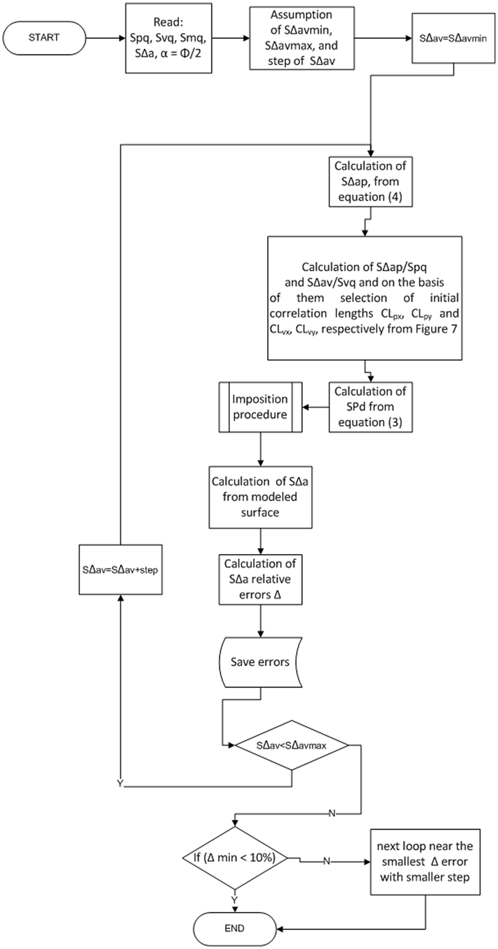
Application of this formula allows the calculation of the average slope of the plateau surface part SΔap for a known slope of the resultant (measured) surface SΔa, the Spq, Svq and Smq (or Spd) parameters and assumed slope of the valley part SΔav. Figure 10 presents a scheme of modelling plateau-honed surface topography with a given arithmetical slope. In this procedure minimum and maximum values of the SΔav slope and SΔav slope increment (step) were assumed. For a known value of the average slope of the measured surface SΔa and an assumed value of the slope of the valley part SΔav one should calculate the slope of the plateau surface part SΔap from equation (5). For given slopes SΔap and SΔav, as well as the honing angle α, the correlation lengths CLpx and CLpy, as well as CLvx and CLvy of the initial one-directional plateau and valley surfaces (before rotation) of the Gaussian ordinate, distribution can be obtained from a drawing similar to Figure 7. Figure 7 was achieved using the Sq parameter value of 1 µm. Because the average slope of a surface is proportional to the standard deviation of its height, the SΔap slope should be divided by the Spq parameter and SΔav by the Svq parameter. The received slopes SΔap/Spq and SΔav/Svq are then equal to the SΔa parameter in Figure 7, and on this basis, initial correlation length estimations CLpx and CLpy, as well as CLvx and CLvy, can be obtained from a drawing similar to Figure 7, for measured sampling intervals. After the imposition procedure, the relative errors Δ of slope SΔa of the modelled surface, in comparison with the measured surface, was calculated and stored. Next, the slope SΔav increased by a step and the described procedure was repeated until a maximum value of the valley slope was reached. Then, if the relative errors Δ was smaller than 10%, the modelling procedure was finished. Otherwise, the next loop should be done with valley slope SΔav close to the value for the smallest Δ error of the resultant slope with a smaller step increment. Figure 10 presents the basic scheme of obtaining a two-process surface with a given arithmetical slope. One should remember that other parameters of the modelled surface should be similar to those of the measured one.
Flow chart of 3D surface topography modelling with a given slope SΔa.
The results of 3D surface topography modelling
Figure 11 shows average values of the absolute relative errors of plateau-honed 3D cylinder liners surface topography parameters. In the majority of cases (about 80%) modelled surfaces had higher values of Sa and Sq parameters than measured surfaces. By contrast, maximum height of the modelled surfaces, described by Sz and S10z parameters, was usually smaller than that of the measured surfaces. This is the effect of the existence of non-statistical summits and valleys on the measured surface (outliers). Similarly, the values of Sp and Sv parameters of the simulated surfaces were smaller than those of the measured surface. Since the Spq, Svq and Smq parameters were input values in the model, their errors were comparatively small. However, inaccuracies in parameters from the Rk group determination were larger. Values of the parameter Sr2 of the modelled surfaces were higher than those of the measured surfaces. The values of the Str parameter and PΔac/PΔaa of modelled surfaces were larger than those of measured surfaces. Average deviations of SΔa and SΔq parameters determination were small, but of Spc, larger. Figures 12 and 13 present isotropic views of measured and modelled surfaces. Selected values of parameters are also given. Std means texture direction (ISO 25178). 46
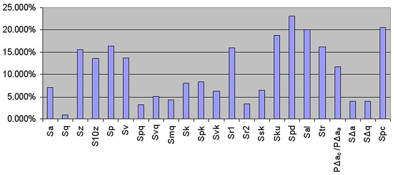
Average values of absolute relative errors of plateau-honed 3D cylinder liners surface topography parameters.
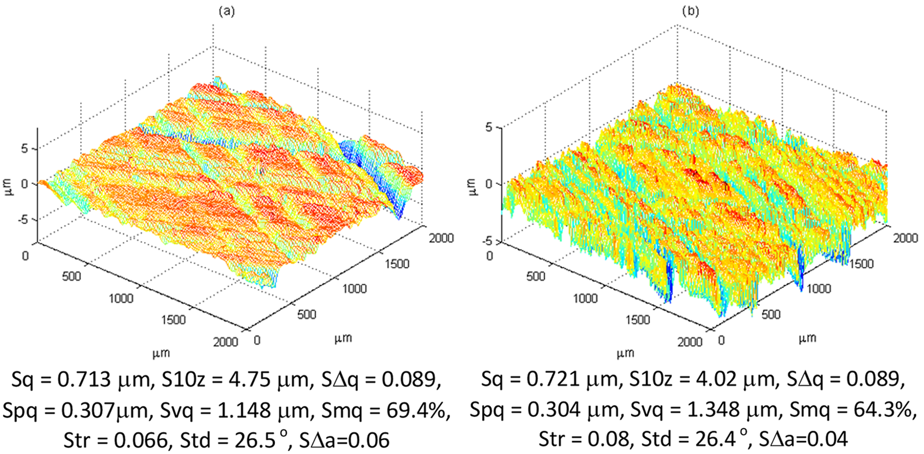
(a) measured surface topography; (b) modelled surface topography of plateau honed cylinder.
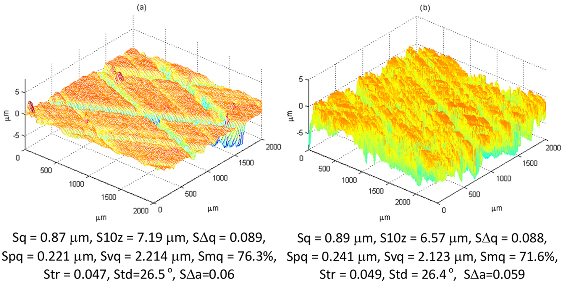
(a) measured surface topography; (b) modelled surface topography of plateau honed cylinder.
Conclusions
Two-process 2D profile and 3D (areal) surface topography after plateau honing can be computer-generated by imposition of smooth on rough structures of the Gaussian-ordinate distribution. This method is better than the two other methods of non-Gaussian surface modelling presented in the technical literature. The original procedure was developed in order to obtain prescribed values of the following parameters of the modelled profile: plateau height Ppq, valley height Pvq, material ratio at plateau-to-valley transition Pmq, skewness Psk and correlation length CL. In this procedure, optimization was done automatically using a two-objectives optimization technique in order to minimize differences between correlation length and skewness of modelled and measured profiles. The mating accuracy was good, taking into account the complicated character of plateau-honed cylinder profiles. The other parameters were also analysed. Discrepancies between horizontal parameters of modelled and measured profiles were comparatively large.
This procedure can be extended into 3D. Dependence connecting the arithmetic average slope of the modelled areal surface topography with slopes of plateau and valley texture parts (weighted by their fractional area contribution) can be helpful in reducing calculation time. The differences between the following parameters of modelled and measured surface topographies were minimized: standard deviation of plateau part Spq, standard deviation of valley part Svq, material ratio at plateau-to-valley transition Smq, arithmetical average slope SΔa, summit density Spd, mean summit curvature Spc, skewness Ssk and ratio of profile average slopes in perpendicular directions PΔac/PΔaa. An original procedure of obtaining two-process plateau-honed cylinder surface topography with a given slope was presented. The other parameters were also taken into consideration. The selected method could be properly applied for simulation of plateau-honed cylinder texture. The modelling procedure allowed a correct estimate of parameters: Sa, Sq, Ssk, SΔa, SΔq, Spq, Svq and Smq. The errors of determination of parameters Sal, Str, Sds and Spc were higher. Discrepancies between parameters from the ISO 13565-2 44 standard were larger than those from the ISO 13565-3 42 standard both in 2D and 3D.
Footnotes
Acknowledgements
The authors wish to thank Professor J-J Wu for providing his software.
Funding
This research received no specific grant from any funding agency in the public, commercial, or not-for-profit sectors.