Sage Journals: Discover world-class research

Abstract

Web surveys are becoming increasingly popular but tend to have more breakoffs compared to the interviewer-administered surveys. Survey breakoffs occur when respondents quit the survey partway through. The Cox survival model is commonly used to understand patterns of breakoffs. Nevertheless, there is a trend to using more data-driven models when the purpose is prediction, such as classification machine learning models. It is unclear in the breakoff literature what are the best statistical models for predicting question-level breakoffs. Additionally, there is no consensus about the treatment of time-varying question-level predictors, such as question response time and question word count. While some researchers use the current values, others aggregate the value from the beginning of the survey. This study develops and compares both survival models and classification models along with different treatments of time-varying variables. Based on the level of agreement between the predicted and actual breakoff, we find that the Cox model and gradient boosting outperform other survival models and classification models respectively. We also find that using the values of time-varying predictors concurrent to the breakoff status is more predictive of breakoff, compared to aggregating their values from the beginning of the survey, implying that respondents’ breakoff behaviour is more driven by the current response burden.

Keywords

breakoff timing time-varying variables Cox model LASSO Cox model logistic regression random forest gradient boosting support vector machine

Introduction

Web surveys have become one of the most important tools for social scientists, a trend that has been accelerated by the Covid-19 pandemic. However, running surveys on the web has some limitations, one of which is the high survey breakoff (Tourangeau et al., 2013). Survey breakoff happens when the respondent starts the survey but does not complete it (Lavrakas, 2008). Consequently, the sample size available is reduced, and survey estimates can be biased when those that break off differ from those that complete the survey.

There are two main approaches to mitigating the damage of breakoffs. The first one is reactive. The differential breakoff propensity can be corrected via weighting after the data collection (Steinbrecher et al., 2015). The other is minimising the breakoff during data collection. For example, a model can continuously monitor the breakoff risk during the response process and trigger some interventions (e.g., displaying motivation messages) when the respondent is predicted to break off soon (Mittereder, 2019).

For both post-hoc correction and real-time intervention, a good prediction model of the breakoff is essential. Such a model would identify the factors strongly associated with the breakoff propensity and make weighting more effective. Also, a good prediction of the breakoff risk would help activate the intervention at the most relevant timing and potentially increase its efficiency.

The Cox survival model is widely used when studying survey breakoffs (Chen et al., 2022; Hochheimer et al., 2016; Mittereder, 2019; Peytchev, 2009) as not breaking off implies “surviving” the response process. Previous research has shown that this traditional model can achieve a relatively satisfactory prediction accuracy (e.g., 78% for Mittereder, 2019). However, there is a growing interest to go beyond traditional statistical models and use machine learning to improve the prediction performance even further (e.g., Lee & Lim, 2019; Spooner et al., 2020). Currently, there is scant application of survival machine learning in predicting survey breakoffs. Against this backdrop, the present study will first compare the survival machine learning models with the traditional Cox model to investigate whether the former improves the performance of breakoff prediction.

Meanwhile, classification models, another class of machine learning, is widely used in survey nonresponse prediction (e.g., Kern et al., 2019; Liu, 2020) but never applied to breakoff prediction. Models of this class usually treat each row in the data as independent. We will compare five classification models to see how they perform with regards to predicting breakoffs in the data where the rows are not independent from each other (i.e., questions in the row are clustered by respondents). These five models are: traditional and LASSO logistic regression, random forest, gradient boosting, and support vector machine. Finally, we will compare the best performing survival model with the best performing classification model to investigate whether considering the clustered data structure by the survival model improves the breakoff prediction performance.

In addition to the statistical model used, what predictors are included and the way they are coded also plays a crucial role in the model prediction performance (Kuhn & Johnson, 2013). Unlike time-constant predictors (e.g., socio-demographic variables), there is no consensus in the existing literature regarding how to treat the time-varying variables (e.g., question response time and question word count). In fact, three different treatments were used in prior studies of survey breakoffs: using the variable as it was originally coded (i.e., concurrent with the outcome) (Vehovar & Cehovin, 2014), lagged (Galesic, 2006) or accumulated (Peytchev, 2009). All these treatments are based on different assumptions regarding how the time-varying variable affects breakoffs. For example, a cumulative view of the predictors would emphasise the importance of accumulated burden in a survey while a concurrent coding would emphasise the importance of the variable where breakoff happens. While the treatment of the time-varying variables is essential for the understanding of the causal mechanisms leading to breakoffs as well as the quality of the prediction models, few researchers have explicitly tested which treatment (and the associated assumption) is better, particularly in terms of the model prediction performance. The present study will investigate this by fitting all above models with different coding of time-varying predictors.

The present study will contribute to the existing literature in two ways. First, we will help identify the model that is most predictive of breakoffs and can therefore be used both for real-time interventions and to generate weights for breakoff adjustments. Second, by investigating different ways of using time-varying predictors, this study will contribute to the theoretical debate regarding the process leading to breakoffs.

Literature Review

Real-Time Intervention in Web Surveys

Breakoffs are common in web surveys. For example, Revilla (2017) reviewed 185 opt-in web surveys distributed through a Spanish survey company and reported a mean breakoff rate of 11.8%. In another meta-review, Liu and Wronski (2018) documented an average breakoff rate of 13% across the 25,000 non-probability web surveys implemented in SurveyMonkey.

Given the prevalence of breakoffs, survey researchers have devoted attention to studying the breakoff as a specific outcome of interest and found a number of important predictors. Some examples are using the small-screen device to answer the survey (Lugtig & Luiten, 2021) or implementing technically complicated features in the survey (Funke et al., 2011). Based on the identified factors, researchers usually propose changes in designs that are prone to breakoffs, such as optimising the survey for mobile devices (Mavletova & Couper, 2015). However, most proposed solutions are reactive, meaning that survey practitioners can only make changes after data collection. In this case, proactive solutions may offer a better alternative to mitigate the damage of breakoffs. One example of proactive solutions is the real-time intervention in web surveys (Kreuter, 2017). Such systems have been implemented in surveys and proved to be useful, for example by discouraging respondents from speeding through the questionnaire (Conrad et al., 2017).

The study of Mittereder (2019) is one of the few that used a proactive approach in the context of discouraging survey breakoffs. She implemented a model in a survey that continuously calculated the breakoff risk at the page level for each respondent. When the model predicted a breakoff risk that was higher than a pre-set threshold, a message appeared and highlighted the importance of completing the entire questionnaire. Prior to the survey, the sampled members were randomly assigned to three groups where the timing of displaying the message varied. The control group never had a pop-up message (i.e., no intervention) while the generic group saw the intervention message immediately at the first question (i.e., intervening irrespective of the breakoff risk). Respondents of the tailored group only received the pop-up message when the model predicted a high likelihood of quitting in the next question (i.e., intervening at the highest breakoff risk). When comparing the control group with the other two, the study found that the message was effective in lowering the breakoff rate among some specific respondents, such as students and females.

The review so far highlights the potential of the real-time intervention system in web surveys. Using such a system to effectively combat breakoffs has three pre-requisites: (1) the model can accurately predict the breakoff risk at the question level, (2) variables in the model are predictive of the imminent breakoff and (3) the interventions are effective in discouraging breakoff. Nevertheless, there is limited research in all three areas currently. The current study will explicitly tackle the first two aspects.

Models of web survey breakoffs

The Cox survival model is commonly used in the study of survey breakoffs (Chen et al., 2022; Hochheimer et al., 2016; Mittereder & West, 2021; Peytchev, 2009). This model estimates the breakoff hazard which is defined as the probability of a person breaking off at a specific question given that this person has not experienced this event before (Mills, 2011). Previous research has shown that the Cox model can give a relatively satisfactory prediction performance. For instance, the study of Mittereder (2019) reviewed above reported that 78% of survey pages were correctly predicted to be (non-)break pages.

Despite the achievement of traditional statistical models, data-driven machine learning models are increasingly being used. One explanation for this change is that the traditional statistical models always include all input predictors even though some predictors are not associated with the breakoff hazard. Including many irrelevant predictors in the model can lead to overfitting and poor model interpretability (Tibshirani, 1997). In contrast, some machine learning models have a built-in feature of automatic predictor selection, which helps exclude predictors that contribute little or none to the outcome prediction (Wang et al., 2019). Another reason for the movement to the machine learning models is that those models are usually non-parametric, meaning that users do not need to make prior specification about the relationship between the outcome and the input predictors as the traditional statistical models require (Buskirk et al., 2018). Such flexibility in the model form can reduce the chance of the model misspecification and thus has potential for improving the model prediction performance.

However, there is currently little research regarding the potential of survival machine learning models in survey research (including breakoff prediction). Against this backdrop, the first research question of this study is:

RQ1

Do survival machine learning models predict web survey breakoffs more accurately than the traditional Cox survival model?

In contrast to the scant application of survival machine learning models in survey research, classification models, another class of machine learning, are increasingly used in modelling survey nonresponse. Indeed, many survey researchers have documented that classification machine learning models could predict survey nonresponse more accurately, compared to the traditional logistic regression. Some examples of the classification models fitted in those studies are LASSO logistic regression (Liu, 2020; Signorino & Kirchner, 2018), support vector machines (Kirchner & Signorino, 2018), random forest (Buskirk, 2018) and gradient boosting (Kern et al., 2021).

However, unlike survival models, most classification models cannot handle the clustered structure in the survival data. To be more specific, many predictors of survey breakoffs (especially those question-level predictors) are time-varying, such as the question word count and question response time. To accommodate such predictors in the breakoff study, the long data format (where a row is a combination of respondents and questions) has to be used. This clustered structure (questions are clustered within respondents) means that some rows are dependent. This is different from the wide format (a row represents a unique respondent) where the classification models can easily treat each row as independent observations. Studies mentioned earlier already demonstrate that classification models can produce good prediction in the wide data, but it is unclear whether those models can still perform well when there is clustering in the data (and if so what is the best model among them). Thus, the second research question of this study is:

RQ2

What is the best classification model for predicting web breakoffs in clustered data?

If the ultimate goal of the researchers is to have a good prediction model for better survey weighting or breakoff intervention, survival models and classification models are two available options. Both classes of models approach the task of prediction differently and have its own merits, but one question remains unanswered is which of them can predict breakoff more accurately. On other one hand, accounting for the clustered structure in the data makes survival models more in line with the data generating process (Singer & Willett, 2003), which is expected to produce more accurate breakoff prediction. On the other hand, classification models focus primarily on finding the pattern between predictor values and the breakoff event and then use such a pattern to make predictions on new data. Currently, no researcher has compared survival models and classification models in the context of survival data to investigate whether respecting the clustered data structure is useful for breakoff prediction. The third research question will bridge this gap:

RQ3

Does the best performing survival model predict web survey breakoffs more accurately than the best performing classification model?

Predictors of Web Survey Breakoffs

In addition to comparing different models for breakoff prediction, this study will also investigate how different types of variables affect breakoff, with a specific focus on the time-varying predictors. In the literature about breakoffs, a wide range of predictors are usually explored, but all of them can be grouped into time-constant and time-varying predictors. The former includes predictors whose values do not change throughout the questionnaire. Examples are features implemented at the survey level (e.g., the survey displays the progress bar or not) (Villar et al., 2013) and respondent characteristics, such as gender (Peytchev, 2011) and education (Blumenberg et al., 2018). On the other hand, values of predictors in the time-varying group change from question to question, such as the number of characters in the question (Tijdens, 2014).

As the value of the time-constant variables always remains the same, researchers can directly include this type of variable in the model. However, for the time-varying variables, there are different approaches to include them in the modelling. Each approach is based on different assumptions about how the time-varying variable affects breakoffs.

At one extreme, some researchers accumulate the values of the time-varying variables from the start of the survey until the respondent breaks off. Supporters of this approach assume that breakoffs are caused by the gradual accumulation of burden from the beginning of the survey. An example of the variable coded in this approach is the cumulative number of questions the respondent has seen since the start of the survey (Peytchev, 2009).

Another approach of treating the time-varying variable involves no processing at all but using the original coding of the variable. In this case, researchers implicitly assume a concurrent effect of the variable: some factors are so burdensome that their presence is likely to result in a breakoff event. When including time-varying variables in the model of breakoffs, researchers use the predictor value that is concurrent with the outcome. An example is the use of a binary variable which indicates whether or not the survey page signifies more incoming questions (Vehovar & Cehovin, 2014).

Other strategies that have also been used in the past are in between the two treatments we discussed so far. One example is using the lags of the time-varying predictors. Like the accumulation approach, lagging assumes that the past event influences the breakoff likelihood. However, this approach further assumes that the recent event (as opposed to all events in the past) matters the most in breakoff prediction. For instance, Galesic (2006) used respondent’s self-reported interest and burden of the previous question block (a block consists of multiple questions of the same topic) to explain their breakoffs at the next block. In this case, the lagged-one value of the time-varying variable was used.

In summary, researchers have different assumptions regarding how the time-varying variables impact breakoffs, which in turn determines the way they treat the time-varying variable in statistical models. However, little research has been conducted to explicitly compare these different treatments of the time-varying variables (and the associated underlying assumptions), especially in the context of breakoff prediction. As a result, this study will compare three different treatments of the time-varying predictors: using either only cumulative or concurrent coding and using both simultaneously. By comparing the prediction performance resulted from these different treatments, the study will answer the fourth research question:

RQ4

What is the best way to treat time-varying predictors of breakoffs in order to maximise the prediction performance?

Data

The data used in this study comes from a repeated, cross-sectional and non-probability web survey about respondents’ spending on clothing, utilities bills and non-health insurance (Eckman, 2021). The survey was administered to the members of the Lightspeed Panel, an opt-in web panel in the United States. Upon completing the survey, the respondents received points which can be accrued and redeemed later. Two waves were collected. The first wave was conducted between September and October 2019 while the second was collected in October 2020. The majority of the respondents in both waves are not students (around 70%), have a degree at the college level or above (70%) and belong to the white ethnicity group (74%). The proportion of married respondents is roughly the same as the unmarried ones. Respondents in the first wave tend to be younger than those from the second wave (an average of 43 vs. 48). Although the first wave survey has more questions than the second one (196 vs. 126), the respondents of both waves spent, on average, approximately 11 minutes in the questionnaire before survey breakoff or completion.

The survey is considered appropriate to analyse for three reasons. First, it recorded the outcome of interest, namely breakoffs. Out of the 3128 and 2370 respondents in the first and the second wave, 520 and 403 quit the survey without completing it, resulting in a breakoff rate of around 17% for both waves. Furthermore, the survey recorded the last question respondents completed, meaning that the breakoff position is known. More importantly, the breakoff pattern of both waves is very similar. As can be seen in Figure 1, the highest breakoff hazard happened at the beginning of the survey for both waves. The second peak occurred after 10 to 15 questions, and questions within this range either involve sensitive topics (i.e., rent/mortgage for the dwelling), belong to matrix questions or introduce a new series of topics. The second peak occurred few questions earlier in Wave 2 simply because some questions were not asked in this wave, bringing forward those sensitive and matrix questions and the associated second peak. After the second peak, the breakoff hazard in both waves tapered off. All peaks after the 100th questions in Wave 1 were mainly due to the continually decreasing sample size involved in the breakoff hazard calculation (206 respondents remained in the survey at the 115th question compared to over 3000 respondents when the survey started). The similar breakoff pattern across waves means that we can mix data of both waves when training and testing models.

Figure 1.

Change in the breakoff hazard by the number of questions seen for each wave.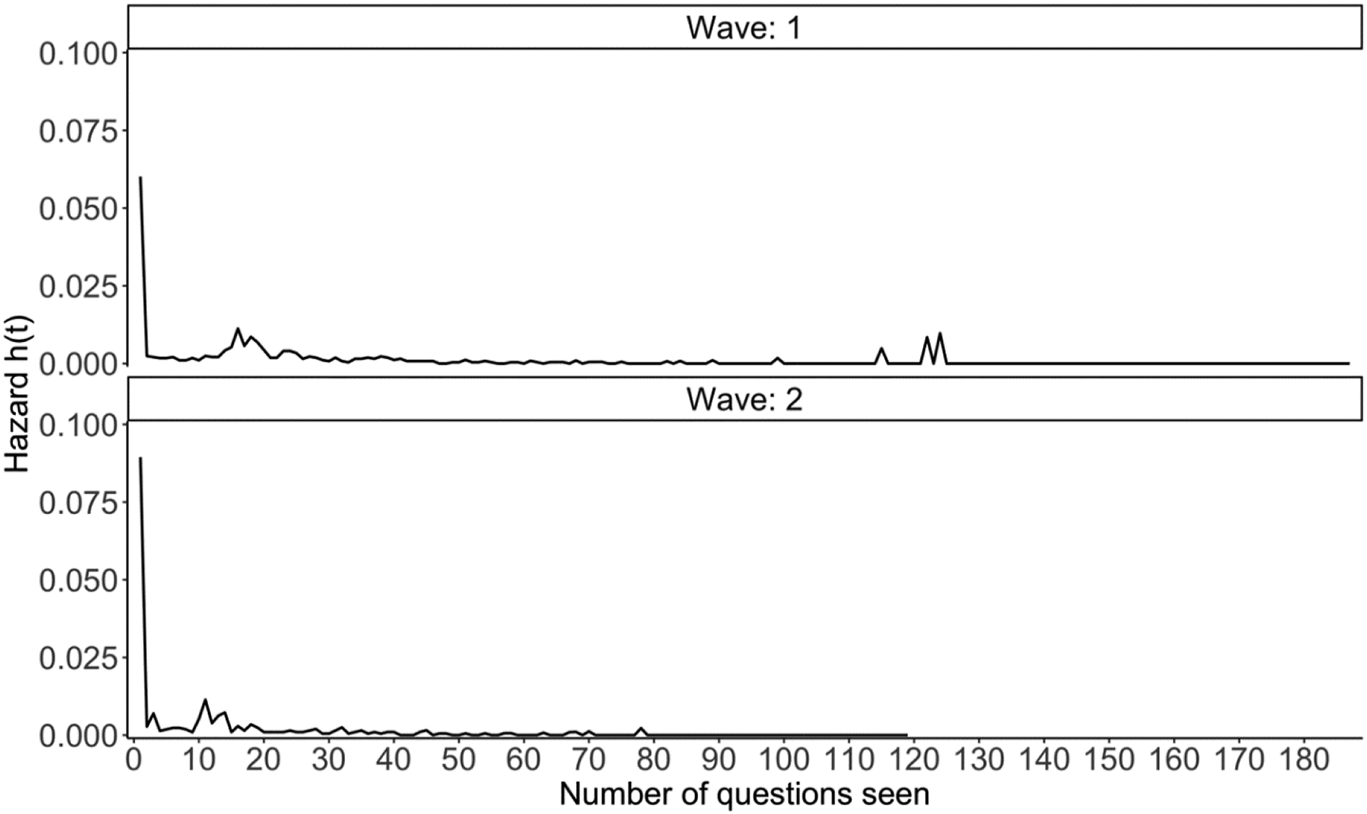

As the survey was initially conducted to answer questions about specific survey designs, three experiments were embedded in it. The first two experiments described below were implemented in both waves, but the third experiment was only carried out in Wave 2.

The first experiment is about the filter question format. The filter question is a type of question that can trigger some follow-ups when answered positively. For example, answering “yes” to the filter question “Have you bought any jacket in the past 12 months” will activate a set of questions such as “Where did you buy it” and “How much did it cost”. There are two formats for asking filter and follow-up questions, namely the grouped and interleafed format. In the grouped format, respondents see all filter questions of one particular topic (e.g., cloth items) together before moving to the follow-ups. On the other hand, individuals responding to the interleafed format are immediately exposed to the follow-ups if they answer “yes” to the filter questions. Depending on the question block, there were five to six filter questions, each of which could trigger four to five follow-up questions. Respondents were randomly assigned to one of the two formats.

The second experiment is related to the order of the question topic. In each wave, there were six question blocks: demographics, housing, clothing, utilities, non-health insurance and income. The first question block (Block 1) always asked respondent’s demographics followed by the characteristics of their housing unit (Block 2). Questions about respondent’s household income were always shown in the last question block (Block 6). Respondents’ clothing purchase, utility payment and non-health insurance were randomly assigned to one of the remaining blocks (Block 3, 4 and 5). This randomisation created six possible block orderings, and respondents were randomly allocated to one of the orderings.

The third experiment (present only in Wave 2) is concerned with the order of the questions within the randomised blocks (Block 3, 4 and 5). In the first wave, the position of questions in all six blocks was fixed. In the second wave, while the order of the questions within Block 1, 2 and 6 still remained the same, the questions within Block 3, 4 and 5 were ordered in one of the two ways: (1) high-frequency to low-frequency and (2) low-frequency to high-frequency. The frequency is determined by how often the respondents selected a “yes” for the filter questions in Block 3, 4 and 6 in the first survey wave. Again, respondents were randomly assigned to one of the two groups.

All three experiment designs were crossed, so the respondents could only be in one of the 12 experimental groups in the first wave (2 filter question formats $\times$ 6 block orders) and one of the 24 experimental groups in the second wave (2 filter question formats $\times$ 6 block orders $\times$ 2 question orders).

Method

Two classes of models are fitted in this study (See Table 1), and both are applied to the long data (where questions are clustered by respondents) in this study to predict breakoff at the question level. The first class is the survival model, which can predict the probability of a respondent breaking off conditional upon no prior breakoff event for this respondent. The traditional Cox model and LASSO Cox belong to this class of model and are fitted in this study. Differently, models of the second class ignore the clustering of questions per respondent in the data, so they will consider each record in the data as a separate respondent and predict the probability of that record in the data having a breakoff event independently from all other records. We denote such a model class as the classification model, and five of them are fitted in this study: traditional and LASSO logistic regression, support vector machine, random forest and gradient boosting.

Table 1.

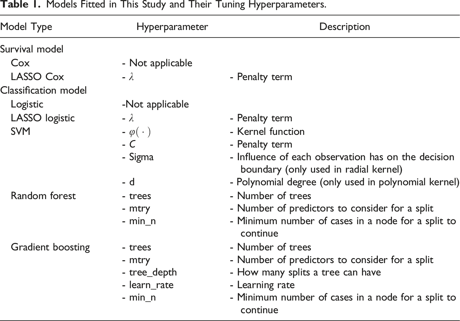
Models Fitted in This Study and Their Tuning Hyperparameters.

Model Type	Hyperparameter	Description
Survival model
Cox	- Not applicable
LASSO Cox	- $λ$	- Penalty term
Classification model
Logistic	-Not applicable
LASSO logistic	- $λ$	- Penalty term
SVM	- $φ (·)$	- Kernel function
	- $C$	- Penalty term
	- Sigma	- Influence of each observation has on the decision boundary (only used in radial kernel)
	- d	- Polynomial degree (only used in polynomial kernel)
Random forest	- trees	- Number of trees
	- mtry	- Number of predictors to consider for a split
	- min_n	- Minimum number of cases in a node for a split to continue
Gradient boosting	- trees	- Number of trees
	- mtry	- Number of predictors to consider for a split
	- tree_depth	- How many splits a tree can have
	- learn_rate	- Learning rate
	- min_n	- Minimum number of cases in a node for a split to continue

Traditional Cox Model

As mentioned earlier, predicting survey breakoffs is essentially a survival problem, and the traditional Cox model is designed to handle the survival data. It can explain whether breakoff will happen and if so its timing (Singer & Willett, 2003). We code the timing as the number of questions seen by respondents up to the point where they broke off or completed the survey, which is an approach commonly used in the prior literature (Chen et al., 2022; Mittereder & West, 2021; Peytchev, 2009).

As shown in its equation below, the breakoff hazard at a specific time t is modelled as the product of the baseline hazard 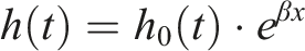$h_{0} (t)$ (i.e., the breakoff risk when all predictor values are zero or at the reference level) and the predictor’s multiplicative effect $β$ on the breakoff hazard.

h (t) = h_{0} (t) · e^{β x}

To estimate the coefficients $β$ , the partial likelihood is used. For computational efficiency, the negative log transformation of the partial likelihood is actually estimated, and the algorithm will identify the combination of parameters that minimises the negative log likelihood. Given the popularity of the Cox survival model in estimating breakoff risks, it is used as a benchmark for other survival models fitted in this study.

LASSO Cox

LASSO Cox builds on the traditional Cox survival model by adding a penalty term to the negative log likelihood estimate to penalise those models that have many parameters (Tibshirani, 1997). The penalty term $λ$ is a non-negative hyperparameter and controls the degree of penalisation. When $λ$ is zero, no penalisation is imposed, and the fitted model is the same as the traditional Cox model. The larger the $λ$ the more estimated model coefficients are shrunk towards zero. Some of the coefficients will be equal to zero when $λ$ is large enough and they will be excluded from the final model. This automatic predictor selection is especially useful for complex models where there are a large number of predictors. The LASSO Cox model is used in this study to see whether a simpler model would outperform the full-size Cox survival model.

Support Vector Machines

Like LASSO Cox model, the support vector machine (SVM) also uses a penalty term and aims to minimise a defined function. Despite this similarity, SVM operates very differently. It tries to find a hyperplane in the high-dimensional space defined by the number of predictors such that the breakoff and non-breakoff respondents, represented as points in the space, can be linearly separated (Rhys, 2020). Given that there might be many hyperplanes that could perfectly separate the two classes, the best one must satisfy two criteria. It should be farthest from the points of both classes, and points of one class (y = 1) lie above this hyperplane while points of the other class (y = −1) fall below it.

However, two classes (in this case respondents who complete and break off the survey) are rarely perfectly separable by a linear plane in practice. SVM addresses this issue in two ways. Firstly, users can extend the space by transforming the predictors. The transformation is equivalent to adding more dimensions to the data, which makes the data linearly separable in the enlarged dimensions. The function for the transformation is called the kernel $φ (·)$ . Some commonly used kernels are linear kernel (i.e., no transformation), polynomial kernel (e.g., quadratic) and radial kernel. The second approach for finding a linear separating hyperplane is allowing some misclassification (i.e., the respondent is predicted by the model to be a breakoff case though the reverse is true). The extent of allowed misclassification is controlled by a non-negative penalty term $C$ . Larger $C$ will impose more penalty on the misclassification and push the fitting algorithm to work harder to produce more correct classification.

The kernel function $φ (·)$ and the penalty value $C$ are the two hyperparameters in SVM. Using the hyperplane with the tuned hyperparameters, the respondents can be classified as breakoff or non-breakoff cases depending on which side of the hyperplane they are predicted to fall into.

Random Forest

Both random forest and gradient boosting require fitting multiple decision trees. Based on the breakoff status, the decision tree recursively partitions the respondents into two child nodes using one of the input predictors. As such, respondents within the same node become more homogeneous in terms of their breakoff status while respondents between nodes are more dissimilar (Buskirk et al., 2018). Gini index quantifies the heterogeneity of a node based on the proportion of breakoff and non-breakoff respondents in the node. The higher the Gini index the less homogeneous (or more heterogeneous) the cases in the node are. By comparing the Gini index of a parent node with that of the child nodes resulted from using different predictors to split the tree, the decision tree will choose the predictor which can make the largest reduction in the Gini index compared to the parent node. The splitting process will stop according to some user-defined criteria such as the minimum number of respondents required in a node for making a further split (Rhys, 2020).

Although the random forest and boosting are based on the decision tree, the way they develop a single tree slightly deviates from the fitting process described above. The random forest incorporates two randomised elements into the tree growth. Both randomisations reduce the chance of overfitting and are the two main tuning hyperparameters in random forest. Firstly, rather than using the same data to train the tree model, the random forest will randomly draw B bootstrapped samples from the original data where each of the bootstrapped sample is as large as the original dataset (James et al., 2013). Then, the decision tree is independently developed on each of the B bootstrapped samples. The second randomisation happens when selecting predictors to make a split. Instead of considering all input predictors as the candidate for making a split, only a random subset of the predictors is considered in the random forest (James et al., 2013).

When using random forest to predict the breakoff status, each tree in the forest produces its own prediction (i.e., breakoff or non-breakoff), then the model makes the final prediction by choosing the most frequent predicted breakoff status across all the trees.

Random forest is used in this study for two reasons. First, this model requires little data pre-processing in contrast to others machine learning models, and it can automatically handle some complex model structures (e.g., interactions). Also, most users are familiar with the tree structure, thereby facilitating the interpretability to a degree. All in all, we expect the random forest to strike a good balance between model prediction performance and interpretability.

Gradient Boosting

Like the random forest, gradient boosting also involves fitting multiple trees. However, the two models differ in three main aspects, namely (1) how the fitting algorithm starts, (2) whether the growth of the subsequent tree depends on the preceding trees, and (3) what is the dependent variable.

Specifically, gradient boosting begins by assigning every respondent the same constant (e.g., the average breakoff hazard calculated from the data). The prediction error for each respondent is then simply calculated as the difference between this assigned breakoff hazard and the observed breakoff status (i.e., 0/1). A decision tree is then fitted using the prediction error as the dependent variable. Once this tree is developed, it is combined with the initial average breakoff hazard to make new predictions about the breakoff hazard for all respondents. Taking the difference between the new prediction and the observed breakoff status will lead to a new set of prediction errors, which another tree will proceed to model. This three-step cycle (i.e., fitting trees on the prediction errors, making new predictions by combining the initial average value and all trees fitted so far, and calculating prediction errors) will continue until some user-defined conditions are reached, such as the maximum number of tress allowed.

In gradient boosting, every subsequent tree gradually learns the prediction mistake made by previous ones and improves upon it. Existing literature has shown that the final model from this gradual model development tends to perform better (James et al., 2013). There are many hyperparameters to be tuned in gradient boosting, such as the tree depth (how many splits are performed in a tree) and the learning rate (how quickly the tree learns from the previous mistake). Gradient boosting, SVM and random forest ignore the clustering of the data and it is unclear whether they can improve the breakoff prediction than the two survival models described earlier.

Analysis Plan

To develop and evaluate all the models, we combine both waves of the Lightspeed Panel data and draw a stratified random sample (stratified by wave and breakoff status) with a proportion of 75% of the total rows in the data. These 75% selected rows are used as the training data, and the remaining data are the testing data.¹ All models are built and tuned using the training data, after which the models are applied to the unseen testing data to predict breakoffs at the question level. The level of agreement between the predicted breakoff from the model and the true breakoff status from the testing data forms the basis for evaluating the model performance.

Because the training data are in the long format and many questions do not have a breakoff event (99.75% vs. 0.25%), a class imbalance problem exists. To solve its negative impact on the utility of classification models, we down sample the training data when building the classification models so that the ratio between breakoff and non-breakoff questions is 1:1 (Kuhn & Johnson, 2013). Given that the survival models can handle the clustered data structure, no class balancing is applied to the training data when fitting such models. For survival and classification models, they are evaluated on the same testing data (where no class balancing is carried out). In total, the original training data for developing the survival models have 274,658 rows compared to 1390 rows in the down-sampled training data for developing the classification models. The testing data have 92,952 rows.

To evaluate the performance of the survival models, the concordance index (C-index) is used. This metric quantifies the proportion of respondent pairs in which the breakoff case has a higher predicted breakoff risk (Harrell et al., 1996). The C-index with a value of 0.5 indicates that the model is just as good as the random guess while a value of one means that the model can perfectly distinguish breakoff respondents from those who complete the survey. Because the C-index is specifically designed to work with clustered and imbalanced data (which is the case for the testing data in this study), it will be used primarily to quantify the prediction performance of survival models in this study.

In contrast, there is no guidance on how to evaluate the prediction performance of the classification model when it is applied to clustered and imbalanced data. Therefore, five metrics (Accuracy, Sensitivity, Specificity, Precision and AUC) are used to evaluate the performance of the classification models from different aspects (Kuhn & Johnson, 2013). Accuracy measures the proportion of correctly predicted breakoff and non-breakoff cases out of all available records. Sensitivity and Specificity quantify the proportion of correctly predicted breakoff/non-breakoff cases out of all actual breakoffs/non-breakoff records respectively. Precision is a metric about the proportion of actual breakoff cases out of all the predicted breakoff cases. Differently, AUC (area under the receiving operator curve) is an aggregate metric, which summarises the model performance across different combinations of the true positive rate (also called Sensitivity) and false positive rate (1 - Specificity). All five metrics range between zero and one, and the larger the value the better the model prediction performance is.

As with the development of machine learning models in other studies, we also tune some model hyperparameters. All these hyperparameters are listed in Table 1. We use a random grid search in the tuning where 100 combinations of the hyperparameter values were randomly tried for each model (Kuhn & Johnson, 2013). Tuning is performed using the fivefold cross-validation in the training data. The best hyperparameter value identified via the cross-validation is used when re-fitting the corresponding model on the entire training data. In the end, there are 28 models (7 model types × 4 predictor groups). These 28 models will be evaluated using the testing data.

To answer RQ1 about whether LASSO Cox is better than the traditional Cox model, their C-index values are compared. For RQ2 (what is the best classification models for predicting web survey breakoffs), Accuracy, Sensitivity, Specificity, Precision and AUC are compared among classification models. These five metrics will be used again when answering RQ3 where the outperforming survival model from RQ1 and the outperforming classification model from RQ2 are compared. This is because both classes of the model can generate these five metrics, which ensures that the comparison is on an equal footing.

Unlike the between-model comparison in the first three research questions, answering RQ4 (how different predictor groups affect the prediction performance) will involve within-model comparison. More specifically, the comparison of evaluation metrics is performed across four predictor groups (See Table 2), which is repeated for each of the seven model types mentioned earlier. The prediction performance of the models that only have respondents’ demographic background is treated as the baseline. Time-varying question-level predictors are coded in two ways, namely concurrent and cumulative. Predictors coded in the former way need no pre-processing and are used in the model directly. In contrast, the cumulative coding will aggregate the values of the predictors question by question. For instance, the predictor about the open-ended question will be binary (i.e., whether or not a specific question is open-ended) in the concurrent coding, but the cumulative coding will record how many open-ended questions the respondents have seen so far. By comparing the baseline prediction performance with that of the two models that respectively include the concurrent and cumulative time-varying predictors, we can investigate whether the time-varying predictor groups are more predictive of breakoff and which coding is better. Finally, respondents’ demographic information and both time-varying treatments are simultaneously put into the model to see whether using all available predictors improves prediction performance.

Table 2.

Predictors Used in this Study.

Predictor Group	Predictors
Demographics	Age, education,^a ethnicity, student status,^a marital status,^a filter question format, and question order^a
Concurrent	Responding device, item missing,^a matrix question, open-ended question, question topic, and question word count, filter question format, and question order^a
Cumulative	Item missing (cumulative),^a matrix question (cumulative), open-ended question (cumulative), question topic (cumulative), and question word count (cumulative), and number of times respondents logged into the web survey (cumulative), filter question format, and question order^a
All combined	All predictors above

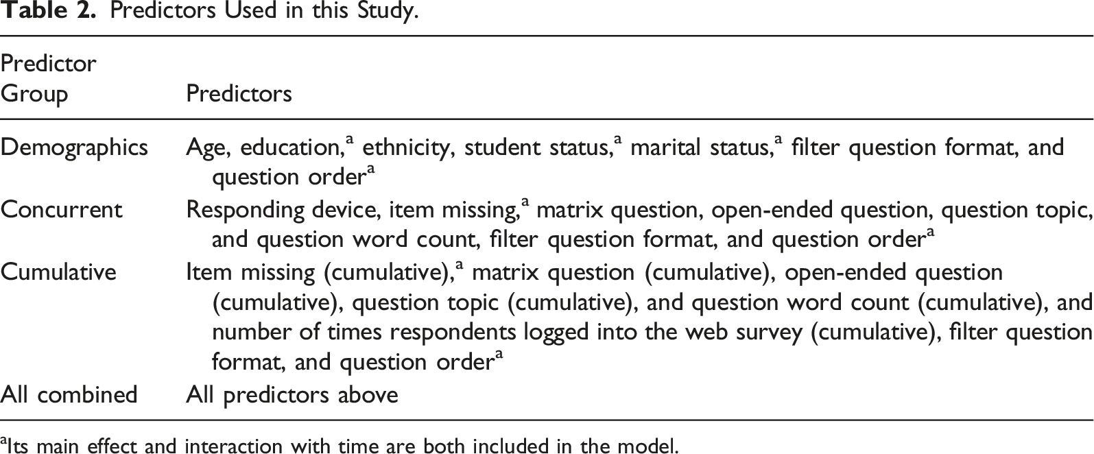
^aIts main effect and interaction with time are both included in the model.

Regardless of which predictor group is used, variables about the two experiments (i.e., filter question formats and question orders of the high-low frequency) are always included in the models as control variables. The variable about the block orders is not included because its information is already represented by the time-varying variable about the question topic. Given that some predictors violate the proportionate hazard assumption of the traditional Cox model, we interact those violating variables with time (i.e., number of questions seen) in all models fitted in this study. Those variables are marked with a subscript in Table 2. The descriptive summary for all predictors in this study and their coding are provided in Supplemental Appendix A.

Results

Comparing Survival Models

Looking at the C-index for the two survival models in Table 3, the traditional Cox model performs better than the LASSO Cox in predicting breakoffs, which holds true for nearly every predictor group. Indeed, traditional Cox can achieve a C-index between 0.68 and 0.85, compared to 0.5 to 0.78 in LASSO Cox. Moreover, the best penalty values in LASSO Cox are very close to zero except for the LASSO Cox fitted using only cumulative time-varying predictors. This implies that there is little need for penalisation and the traditional Cox model is preferred in predicting breakoffs.

Table 3.

Prediction Performance of Survival Models Applied to Testing Data.

Model Type	Predictor Group	Hyperparameter	C-Index
Cox	Demographics	-	0.78
	Concurrent	-	0.74
	Cumulative	-	0.68
	All combined	-	0.85
LASSO Cox^a	Demographics	$λ = 0.00988$	0.78
	Concurrent	$λ = 0.00040$	0.69
	Cumulative	$λ = 2.72$	0.50
	All combined	$λ = 0.00988$	0.78

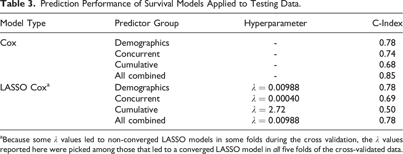
^aBecause some $λ$ values led to non-converged LASSO models in some folds during the cross validation, the $λ$ values reported here were picked among those that led to a converged LASSO model in all five folds of the cross-validated data.

Comparing Classification Models

The next between-model comparison is conducted among classification models. Different metrics to evaluate the prediction performance of those models are presented in Table 4. Looking at the range of all metrics, most of them (except for Precision) are above 0.75, indicating that all the classification models achieve a good prediction performance. Precision is very low, meaning that very few breakoffs predicted by the models are in fact breakoffs and the models raise too many false alarms about breakoff.

Table 4.

Prediction Performance of Classification Models Applied to Testing Data.

Model Type	Predictor Group	Accuracy	Sensitivity	Specificity	Precision	AUC
Logistic	Demographic	0.85	0.62	0.85	0.01	0.85
	Concurrent	0.81	0.73	0.81	0.01	0.87
	Cumulative	0.80	0.70	0.80	0.01	0.84
	All combined	0.84	0.78	0.84	0.01	0.91
	Average	0.83	0.71	0.83	0.01	0.87
LASSO logistic	Demographic	0.85	0.59	0.85	0.01	0.85
	Concurrent	0.81	0.73	0.81	0.01	0.87
	Cumulative	0.77	0.73	0.77	0.01	0.85
	All combined	0.86	0.76	0.86	0.01	0.91
	Average	0.82	0.70	0.82	0.01	0.87
Random forest	Demographic	0.85	0.75	0.85	0.01	0.89
	Concurrent	0.82	0.76	0.82	0.01	0.87
	Cumulative	0.83	0.72	0.83	0.01	0.87
	All combined	0.86	0.76	0.86	0.01	0.91
	Average	0.84	0.75	0.84	0.01	0.89
Gradient boosting	Demographic	0.82	0.79	0.82	0.01	0.90
	Concurrent	0.82	0.77	0.82	0.01	0.88
	Cumulative	0.81	0.72	0.82	0.01	0.86
	All combined	0.85	0.77	0.85	0.01	0.91
	Average	0.83	0.77	0.83	0.01	0.89
SVM	Demographic	0.99	0.55	0.99	0.14	0.84
	Concurrent	0.83	0.69	0.83	0.01	0.86
	Cumulative	0.79	0.69	0.79	0.01	0.84
	All combined	0.83	0.80	0.83	0.01	0.91
	Average	0.86	0.68	0.86	0.04	0.86

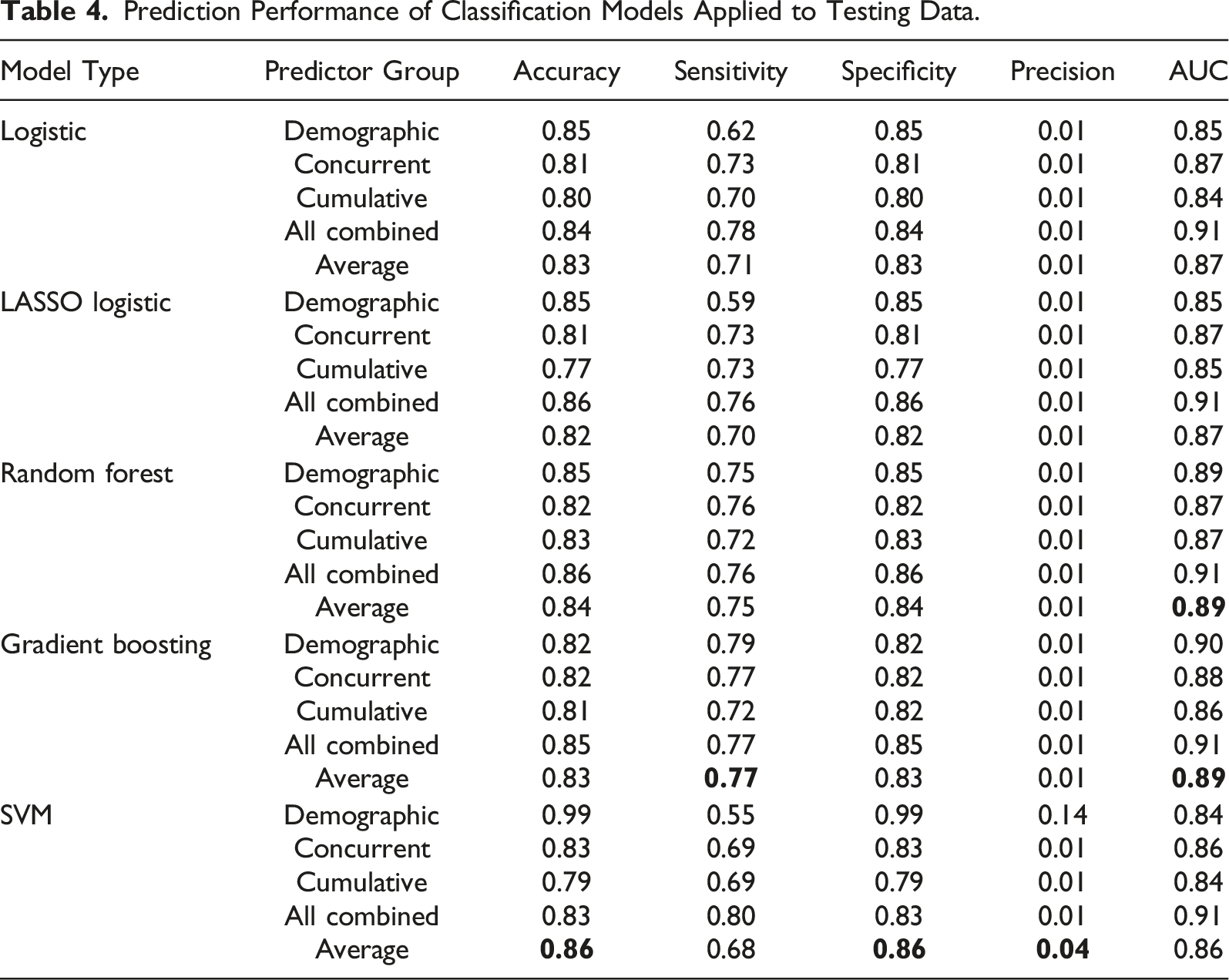
To facilitate the model comparison, the average of different metrics across the four predictor groups is calculated for each model (See the last row of each model type). The highest average metric value across different models is in bold. As can be seen, gradient boosting gives the best prediction performance from the perspective of Sensitivity and AUC. In terms of Accuracy, Specificity and Precision, SVM outperforms the other models.

However, SVM excels in those three metrics mainly because of its performance in the predictor group of demographics alone. More specifically, fitting SVM with only demographics leads to 0.99 in both Accuracy and Specificity, which greatly increases the average value of these two metrics for SVM. However, the Sensitivity of SVM (demographics only) is 0.55, meaning that only 55% of actual breakoffs are captured in the model prediction. Thus, it can be concluded that SVM achieves an overall good prediction performance by simply predicting cases to be non-breakoff most of the time, which comes at the expense of missing many actual breakoffs. In contrast, gradient boosting achieves a good balance across different evaluation metrics. We therefore conclude that gradient boosting outperforms the other classification models. The best hyperparameter values for all models are presented in Supplemental Appendix B.

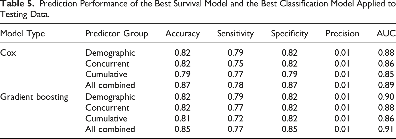
Comparing the Best Performing Survival and Classification Models

Table 5 shows the comparison between the traditional Cox survival model and the gradient boosting classification model (both outperformed other models among their own class). As shown in the table, both models perform equally well as they have similar values in different evaluation metrics. Looking at the AUC, a metric that takes into account both the true positive rate and false positive rate, gradient boosting is slightly better. Given that gradient boosting has no model assumption (in contrast to the proportional hazard assumption in the traditional Cox model), we therefore conclude that extra consideration of the clustering data structure by the survival model might be unnecessary as it does not translate into a significant improvement in the performance of breakoff prediction.

Table 5.

Prediction Performance of the Best Survival Model and the Best Classification Model Applied to Testing Data.

Model Type	Predictor Group	Accuracy	Sensitivity	Specificity	Precision	AUC
Cox	Demographic	0.82	0.79	0.82	0.01	0.88
	Concurrent	0.82	0.75	0.82	0.01	0.86
	Cumulative	0.79	0.77	0.79	0.01	0.85
	All combined	0.87	0.78	0.87	0.01	0.89
Gradient boosting	Demographic	0.82	0.79	0.82	0.01	0.90
	Concurrent	0.82	0.77	0.82	0.01	0.88
	Cumulative	0.81	0.72	0.82	0.01	0.86
	All combined	0.85	0.77	0.85	0.01	0.91

Comparing Predictor Groups

When comparing the prediction performance between different groups of predictors (i.e., within-model comparison), Table 3 (for survival models) and Table 4 (for classification models) together show that using all available predictors frequently results in the highest value in different evaluation metrics. Meanwhile, using the cumulative predictors leads to the worst prediction performance most of the time. However, the performance ranking for demographic and concurrent predictors is less clear as it varies by both the models and the evaluation metrics. Overall, using demographics seems to be more predictive of breakoff than using concurrent predictors.

Discussion

Researchers have discovered that post-collection weighting and real-time intervention are two promising methods to mitigate the impact of breakoffs. The present study extends this line of research by comparing what models are more predictive of breakoffs and thus help derive better weighting and trigger the intervention at the most relevant timing. Also, this study bridges a previous research gap by investigating what variables and how they should be used to maximise the performance of question-level breakoff prediction.

By comparing the C-index of traditional and LASSO Cox models for the survival models, we find that the LASSO Cox does not outperform the traditional Cox (RQ1). This finding is in line with the result from the same comparison but in the medical field (e.g., Lee & Lim, 2019; Spooner et al., 2020). Altogether, it implies that the Cox model is perhaps already flexible enough to create good prediction in the survival context. This can partly be explained by the semi-parametric nature of the traditional Cox model where users do not need to specify the baseline hazard, which reduces the chance of model misspecification. Another possible explanation is that there might not be a large number of predictors in our study to allow the automatic feature selection of LASSO Cox to function properly.

Among the five classification models fitted for the binary classification of breakoffs, we found that gradient boosting gives the best prediction performance across different evaluation metrics (RQ2). This model has been found to be the ‘winner’ in many machine learning comparisons (Bojer & Meldgaard, 2021). The commonly cited reason is that this model focuses on correcting for the prediction errors made by the models in previous iterations (James et al., 2013). Over time, the model will make fewer prediction errors and thus result in better prediction performance.

The most interesting between-model comparison is between the outperforming survival and classification models (RQ3). In our study, it is between the traditional Cox model and gradient boosting. We found that gradient boosting outperforms the traditional Cox model in terms of AUC. This is interesting because researchers who choose to fit the Cox model to the survival data assume that taking account of the clustered data structure will provide more validity to the model. However, our study reveals that gradient boosting, while ignoring the data structure, can still correctly predict many survey questions as (non-)breakoff questions. Equally importantly, gradient boosting can achieve a good prediction performance and not at the expense of model interpretability. Users of the gradient boosting model can still learn what factors are most influential on predicting breakoffs using the variable importance plot or investigate how a specific factor associates with the breakoff risk using the partial dependence plot (Christoph, 2019). We therefore recommend practitioners to deploy the gradient boosting model if their goal is to use real-time interventions to combat web survey breakoffs.

When comparing the prediction performance between predictor types (RQ4), we found that using all available predictors always gives the best prediction performance across different metrics. Given that both the concurrent and cumulative predictors contribute to the prediction, we can conclude that both current burden and the burden accumulated since the start of the survey can cause survey breakoffs. However, using concurrent predictors is better than the cumulative alternative, implying that respondents’ decision to continue or quit the survey is more driven by the question they are exposed to at the moment. We remain cautious about the finding that demographics alone is more predictive of breakoffs than concurrent predictors. This is because we coded the missing demographic information explicitly as a level in the predictor, so respondents who broke off before seeing the demographic questions will always have missing data in demographic-related predictors. Our coding could therefore artificially increase the predictive performance of demographic predictors. Future research can easily solve this issue by using demographics from a sampling frame.

Our study has limitations as well. To begin with, we can only fit one survival machine learning model (i.e., LASSO Cox). This is mainly because existing software packages for fitting survival machine learning models are not mature enough to handle the long data format. Even though the fitting algorithm for LASSO Cox is designed to work with the long data, estimating the LASSO Cox with a lambda value of zero (which in theory is equivalent to fitting a traditional Cox model) led to a non-convergence result while the traditional Cox model converged successfully on the same data. Secondly, we derived most time-varying predictors from the question characteristics (e.g., open-ended, number of words), and there is a limited number of time-varying predictors about respondents’ behaviours (e.g., question response time, mouse back clicks). Prior research has demonstrated that response behaviours can shed more light on the process leading to breakoffs (Mittereder & West, 2021). Future research can explore how different coding of the behaviour-related predictors affects the prediction performance. Lastly, this study cannot investigate whether the lagged version of the time-varying predictors is more predictive of breakoff compared to other coding approaches. This is because creating lags will result in the first few rows of each respondent having missing data in the time-varying predictors. Because some breakoffs happened at the first question, breakoff cases with missing time-varying predictors will be removed and the sample size for model building will be noticeably reduced.

Despite the limitations, our findings can still provide some practical implications. When predicting breakoffs, gradient boosting might be the best candidate model, and concurrent and cumulative coding of the time-varying variables should be simultaneously included as predictors in the model. Future research can extend our study by looking at whether the improved prediction performance leads to better survey weighting and more efficient breakoff interventions.

Supplemental Material

Supplemental Material - Predicting Web Survey Breakoffs Using Machine Learning Models

Supplemental Material for Predicting Web Survey Breakoffs Using Machine Learning Models by Zeming Chen, Alexandru Cernat, and Natalie Shlomo in Social Science Computer Review

Footnotes

Declaration of Conflicting Interests

The author(s) declared no potential conflicts of interest with respect to the research, authorship, and/or publication of this article.

Funding

The author(s) received no financial support for the research, authorship, and/or publication of this article.

Supplemental Material

Supplemental Material for this article is available online.

Note

Author Biographies

Zeming Chen (zeming.chen@manchester.ac.uk) is a PhD candidate in the social statistics department at the University of Manchester. His research focuses on investigating factors impacting survey breakoff and proposing different statistical solutions for this problem. You can find out more about him and his work at:

Alexandru Cernat (alexandru.cernat@manchester.ac.uk) is Associate professor of Social Statistics in the social statistics department at the University of Manchester. His research focuses on: survey methodology, longitudinal data, measurement error, latent variable modelling, new forms of data and missing data. You can find out more about him and his work at:

Natalie Shlomo (natalie.shlomo@manchester.ac.uk) is Professor of Social Statistics in the social statistics department at the University of Manchester. She publishes widely in the area of survey statistics. You can find out more about her and her work at:

References

Blumenberg

Zugna

Popovic

Pizzi

Barros

A. J. D.

Richiardi

(2018). Questionnaire breakoff and item nonresponse in web-based questionnaires: Multilevel analysis of person-level and item design factors in a birth cohort. Journal of Medical Internet Research, 20(12), Article e11046. https://doi.org/10.2196/11046

Bojer

C. S.

Meldgaard

J. P.

(2021). Kaggle forecasting competitions: An overlooked learning opportunity. International Journal of Forecasting, 37(2), 587–603. https://doi.org/10.1016/j.ijforecast.2020.07.007

Buskirk

T. D.

(2018). Surveying the forests and sampling the trees: An overview of classification and regression trees and random forests with applications in survey research. Survey Practice, 11(1), 1–13. https://doi.org/10.29115/sp-2018-0003

Buskirk

T. D.

Kirchner

Eck

Signorino

C. S.

(2018). An introduction to machine learning methods for survey researchers. Survey Practice, 11(1), 1–10. https://doi.org/10.29115/SP-2018-0004

Chen

Cernat

Shlomo

Eckman

(2022). Impact of question topics and filter question formats on web-survey breakoffs. International Journal of Market Research. Online First. https://doi.org/10.1177/2F14707853211068008

Christoph

(2019). Interpretable machine learning: A guide for making black box models explainable. Lulu.

Conrad

Tourangeau

Couper

M. P.

Zhang

(2017). Reducing speeding in web surveys by providing immediate feedback. Survey Research Methods, 11(1), 45–61. https://doi.org/10.18148/srm/2017.v11i1.6304

Eckman

(2021). Underreporting of purchases in the US consumer expenditure survey. Journal of Survey Statistics and Methodology, 124. https://doi.org/10.1093/jssam/smab024

Funke

Reips

U.-D.

Thomas

R. K.

(2011). Sliders for the smart: Type of rating scale on the web interacts with educational level. Social Science Computer Review, 29(2), 221–231. https://doi.org/10.1177/0894439310376896

10.

Galesic

(2006). Dropouts on the web: Effects of interest and burden experienced during an online survey. Journal of Official Statistics, 22(2), 313–328.

11.

Harrell

F. E.

Lee

K. L.

Mark

D. B.

(1996). Multivariable prognostic models: Issues in developing models, evaluating assumptions and adequacy, and measuring and reducing errors. Statistics in Medicine, 15(4), 361–387. https://doi.org/10.1002/(SICI)1097-0258(19960229)15:4<361::AID-SIM168>3.0.CO;2-4

12.

Hochheimer

C. J.

Sabo

R. T.

Krist

A. H.

Day

Cyrus

Woolf

S. H.

(2016). Methods for evaluating respondent attrition in web-based surveys. Journal of Medical Internet Research, 18(11), 1–11. https://doi.org/10.2196/jmir.6342

13.

James

Witten

Hastie

Tibshirani

(2013). An introduction to statistical learning: With applications in R. Springer. https://doi.org/10.1007/978-1-4614-7138-7

14.

Kern

Klausch

Kreuter

(2019). Tree-based machine learning methods for survey research. Survey Research Methods, 13(1), 73–93. https://doi.org/10.18148/srm/2019.v13i1.7395

15.

Kern

Weiß

Kolb

J-P.

(2021). Predicting nonresponse in future waves of a probability-based mixed-mode panel with machine learning. Journal of Survey Statistics and Methodology, 1–24. https://doi.org/10.1093/jssam/smab009

16.

Kirchner

Signorino

C. S.

(2018). Using support vector machines for survey research. Survey Practice, 11(1), 1–14. https://doi.org/10.29115/SP-2018-0001

17.

Kreuter

(2017). Getting the most out of paradata. In Vannette

D. L.

Krosnick

J. A.

Sakshaug

J. W.

(Eds.), The Palgrave handbook of survey research (pp. 193–198). Palgrave Macmillan.

18.

Kuhn

Johnson

(2013). Applied predictive modeling. Springer. https://doi.org/10.1007/978-1-4614-6849-3

19.

Lavrakas

P. J.

(2008). Encyclopedia of survey research methods. Sage Publications. https://doi.org/10.4135/9781412963947

20.

Lee

Lim

(2019). Review of statistical methods for survival analysis using genomic data. Genomics and Informatics, 17(4), Article e41. https://doi.org/10.5808/GI.2019.17.4.e41

21.

Liu

(2020). Using machine learning models to predict attrition in a survey panel. In Hill

C. A.

Biemer

P. P.

Buskirk

T. D.

Japec

Kirchner

Kolenikov

Lyberg

L. E.

(Eds.), Big data meets survey science: A collection of innovative methods (pp. 415–433). John Wiley & Sons. https://doi.org/10.1002/9781118976357.ch14

22.

Liu

Wronski

(2018). Examining completion rates in web surveys via over 25, 000 real-world surveys. Social Science Computer Review, 36(1), 116–124. https://doi.org/10.1177/0894439317695581

23.

Lugtig

Luiten

(2021). Do shorter stated survey length and inclusion of a QR code in an invitation letter lead to better response rates? Survey Methods: Insights from the Field. Online First. https://doi.org/10.13094/SMIF-2021-00001

24.

Mavletova

Couper

M. P.

(2015). A meta-analysis of breakoff rates in mobile web surveys. In Toninelli

Pinter

de Pedraza

(Eds.), Mobile research methods: Opportunities and challenges of mobile research methodologies (pp. 81–98). Ubiquity Press. https://doi.org/10.5334/bar.f

25.

Mills

(2011). Introducing survival and event history analysis. SAGE.

26.

Mittereder

F. K.

(2019). Predicting and preventing breakoff in web surveys. University of Michigan.

27.

Mittereder

West

B. T.

(2021). A dynamic survival modeling approach to the prediction of web survey breakoff. Journal of Survey Statistics and Methodology, 1–34. https://doi.org/10.1093/jssam/smab015

28.

Peytchev

(2009). Survey breakoff. Public Opinion Quarterly, 73(1), 74–97. https://doi.org/10.1093/poq/nfp014

29.

Peytchev

(2011). Breakoff and unit nonresponse across web surveys. Journal of Official Statistics, 27(1), 33–47.

30.

Revilla

(2017). Analyzing survey characteristics, participation, and evaluation across 186 surveys in an online opt-in panel in Spain. Methods, Data, Analyses, 11(2), 135–162. https://doi.org/10.12758/mda.2017.02

31.

Rhys

H. I.

(2020). Machine learning with R, the tidyverse, and mlr. Manning Publications.

32.

Signorino

C. S.

Kirchner

(2018). Using LASSO to model interactions and nonlinearities in survey data. Survey Practice, 11(1), 1–10. https://doi.org/10.29115/SP-2018-0005

33.

Singer

J. D.

Willett

J. B.

(2003). Applied longitudinal data analysis: Modeling change and event occurrence. Oxford University Press.

34.

Spooner

Chen

Sowmya

Sachdev

Kochan

N. A.

Trollor

Brodaty

(2020). A comparison of machine learning methods for survival analysis of high-dimensional clinical data for dementia prediction. Scientific Reports, 10(1), 20410. https://doi.org/10.1038/s41598-020-77220-w

35.

Steinbrecher

Roßmann

Blumenstiel

J. E.

(2015). Why do respondents break off web surveys and does it matter? Results from four follow-up surveys. International Journal of Public Opinion Research, 27(2), 289–302. https://doi.org/10.1093/ijpor/edu025

36.

Tibshirani

(1997). The lasso method for variable selection in the cox model. Statistics in Medicine, 16(4), 385–395. https://doi.org/10.1002/(SICI)1097-0258(19970228)16:4<385::AID-SIM380>3.0.CO;2-3

37.

Tijdens

(2014). Dropout rates and response times of an occupation search tree in a web survey. Journal of Official Statistics, 30(1), 23–43. https://doi.org/10.2478/jos-2014-0002

38.

Tourangeau

Conrad

Couper

M. P.

(2013). The science of web surveys. Oxford University Press.

39.

Vehovar

Cehovin

(2014). Questionnaire length and breakoffs in web surveys: A meta study. 7th Internet Survey Metodology Workshop 2014, Bolzano, Italy, 01 December, 2014.

40.

Villar

Callegaro

Yang

(2013). Where am I? A meta-analysis of experiments on the effects of progress indicators for web surveys. Social Science Computer Review, 31(6), 744–762. https://doi.org/10.1177/0894439313497468

41.

Wang

Reddy

C. K.

(2019). Machine learning for survival analysis: A survey. ACM Computing Surveys, 51(6), 1–36. https://doi.org/10.1145/3214306

Supplementary Material

Please find the following supplemental material available below.

For Open Access articles published under a Creative Commons License, all supplemental material carries the same license as the article it is associated with.

For non-Open Access articles published, all supplemental material carries a non-exclusive license, and permission requests for re-use of supplemental material or any part of supplemental material shall be sent directly to the copyright owner as specified in the copyright notice associated with the article.

0.00 MB

0.13 MB