Sage Journals: Discover world-class research

Abstract

A novel method for defining the measured electrical conductivity of CFRTP in induction heating simulations is presented. This method considers the electrical conductivity’s orientation dependence and accurately predicts electromagnetic and transient temperature fields. The study demonstrates that temperature predictions using the present electrical conductivity model are in good agreement with the experiments, and that it yields improved transient temperature field predictions compared to the other electrical conductivity models.

Keywords

Induction heating anisotropic electrical conductivity fabrics

Introduction

As demand for aircraft continues to grow,¹ the need for cost-efficient production of large composite structures at a rapid rate is ever-increasing. These structures typically consist of several smaller sub-components which can be joined using automated fusion bonding, commonly referred to as welding, when the composites used have a thermoplastic polymer matrix which can be re-melted in the process. Furthermore, if the polymer is reinforced with a carbon fibre material, induction can be used to melt the polymer as the carbon acts as a conductor.

This aforementioned physical principle is utilised in the induction welding technique, which is a key technology employed in the assembly line of the Gulfstream G650 aircraft control surface components.² The components in question are made from a thermoplastic polymer reinforced with a carbon fabric. The current process window for induction welding is defined using empirically determined design guidelines. However, to fully capitalise on the potential of this welding technology and reduce the time-to-market, having the ability to accurately predict the weld line temperature is essential for pre-defining the process window.

Generally, these predictions are made by means of numerical simulations of the electromagnetic field in the total system of inductor (the coil), conductor (in this case, the composite laminate), potentially other objects which are electromagnetically significant in the vicinity of this system (e.g. welding fixture components), and the surrounding air. Subsequently, the Joule heating resulting from these calculations is used as a thermal load in the heat calculation, which in turn is used to calculate the transient temperatures in the composite laminate. A recent study³ developed a numerical method that only requires the modelling of the conductor, significantly reducing the number of elements needed. However, this method does not take into account the influence of the above mentioned electromagnetically significant components outside the domain of the conductor. This is a limitation, as these components can have a significant impact on the overall electromagnetic field.

The electrical conductivity is a key factor in determining the magnitude and direction of induced eddy currents, regardless of the simulation method used. However, accurately defining this property within a predictive computational model remains a challenge. This is shown by previous studies which demonstrated an in-plane anisotropic thermal response of induction heated carbon fabric reinforced thermoplastic composite laminates.^4–7

A straightforward continuum approach, in which an anisotropic electrical conductivity is considered within a three-dimensional Cartesian representation, was found to be effective for thermoplastic polymers with a uni-directional (UD) carbon fibre reinforcement.^8–11 However, this approach cannot predict an in-plane anisotropic thermal response when the reinforcement in the composite is a fabric.

Representations such as those used in Refs. 12–15, which assume a planar uniform isotropic electrical conductivity with the same value along and across the weave, cannot account for the directionality of the induced eddy currents and the resulting thermal response.

Recently, a Finite Element (FE) method was proposed to predict the transient temperatures in a carbon fabric reinforced TPC during an induction heating experiment in which a circularly shaped coil was positioned parallel to a carbon fabric reinforced TPC laminate.^5,6 In this approach, the anisotropic electrical conductivity of each separate ply in the laminate was defined by two, equally thick, stacked, perpendicularly oriented homogeneous UD-layers. Each UD-layer in the ply represented the electrical conductivity in one of the weave directions in the fabric. The electrical conductivity along the fibre direction in the homogeneous layers is calculated according to

σ_{1} = σ_{2} = 0.5 V_{f} σ_{f}

(1)

where V_f is the total fibre volume fraction in the composite and σ_f is the electrical conductivity of the carbon material in the fibres. The electrical conductivities in the two layers were coupled by an electrical conductivity in the fabric’s normal direction, determined via an inverse numerical method based on eddy current measurements. The result is a ‘uniform anisotropic’ electrical conductivity definition which has demonstrated its efficacy in providing accurate temperature predictions for a circularly shaped coil inducing eddy currents in the laminate resembling the coil’s projected shape. However, it is not known if this method is limited in its capacity to accurately predict the temperature when a coil is applied inducing highly oriented eddy currents in the laminate. In the situation described, the choice of which of the UD-layers in the fabric ply is positioned closest to the induction coil is of critical importance. This is because the distance between the coil and the induced material has a significant influence on the predicted temperatures.¹³ In the case of low heating rates, this may not be a limitation, as dissipation of energy in the form of heat conduction which occurs between the virtual UD-layers in the simulations is able to keep up with the heating rate. However, in the case of high heating rates, dissipation cannot keep up with the heating rates, possibly causing inaccurate transient temperature predictions.

This paper examines the potential for improved temperature predictions in induction heating simulations through the use of accurate electromagnetic field approximations. Specifically, the electrical conductivity of a carbon fabric reinforced thermoplastic material (TPC) is defined at the ply level. High heating rates are applied to investigate the generation of eddy currents. This is done to minimise the effects of thermal dissipation in the induced material. Additionally, high heating rates enable welding at high speeds, meeting the need for rapid production rates of large composite structures. Validated measurements of the electrical conductivity are used in the simulations, making them applicable to a range of induction coil geometries. The findings of Ref. 7 are utilised in this research, demonstrating a linear correlation between the measured anisotropic electrical conductivities of a fabric-reinforced TPC material and the heating rate of the TPC to eddy current induction when the directions were highly-oriented.

The heating mechanisms within a TPC laminate can be categorized into three primary types: Joule heating within the fibres, contact resistance losses at the fibre junctions within a fabric ply, and dielectric losses at the fibre junctions between the plies in the laminate. These mechanisms are primarily attributed to the electrical conductance properties of the laminate. The generation of eddy currents requires the presence of conductive loops within the material. In carbon fabric reinforced TPCs, these loops are readily formed within each ply due to the interwoven fibre architecture. The electrical currents flow primarily along the fibres, indicating a Joule heating mechanism. While the fibre bundles of adjacent plies are likely to be in contact, the presence of a resin-rich inter-ply layer hinders the extent of contact, possibly introducing a dielectric heating mechanism. At the intersections of warp and weft fibre bundles, direct fibre contacts are formed, giving rise to contact resistance losses. The presence of a linear correlation between the measured electrical conductivities and heating rate, as reported in Ref. 7, implies that the dielectric heating mechanism is of minimal significance for woven fabric reinforced TPCs under the experimental conditions outlined in Ref. 7. This finding aligns with observations in previous studies, such as Ref. 16.

The objective of this study is thus to provide a method for defining the measured electrical conductivities in induction heating simulations to gain accurate temperature predictions. Additionally, the simulation results using this method are compared to those from simulations using the planar uniform isotropic and the uniform anisotropic electrical conductivity models. The heating rate and maximum temperature are key for welding applications and are hence considered as the most relevant criteria for the present analyses.

Experimental work

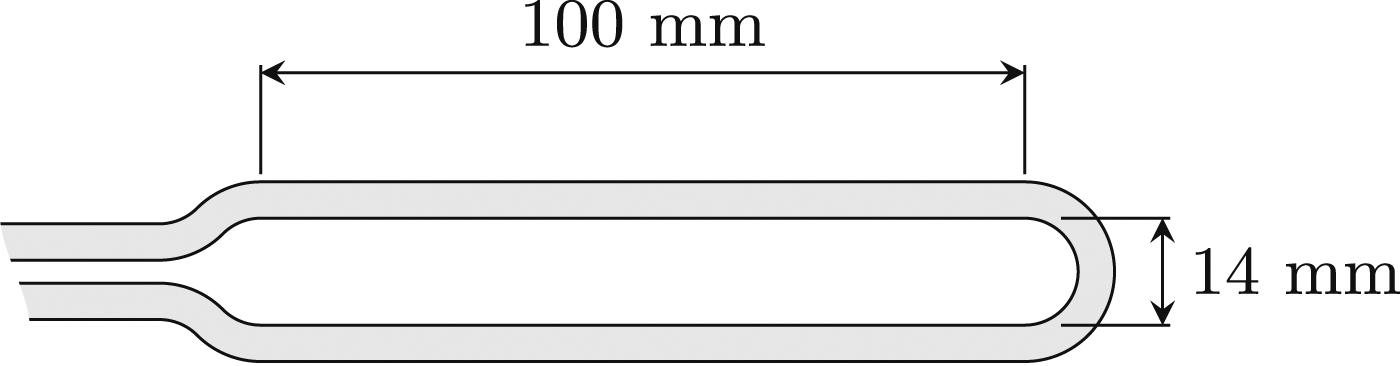
In Ref. 7, an induction heating set-up, which is utilised in the present study, was designed to induce eddy currents in highly oriented, predefined, directions along the coil’s x-direction. A schematic overview of the applied set-up is shown in Figure 1. A water-cooled hairpin shaped coil, manufactured from a 4.8 mm copper tube with 0.8 mm wall thickness, see Figure 2, predominantly generates eddy currents in the laminate in the coil’s length-direction corresponding to the x-direction of the rotated coordinate system in Figure 1. The coordinate system of the plies in the laminate is depicted in Figure 1 as well. The 1- and 2-direction agree with the first two principal directions of the plies while the out-of-plane direction designated by the 3-direction is not depicted.

Figure 1.

Schematic overview of the induction heating set-up.

Figure 2.

Top-view of the applied induction coil. The coil was manufactured using a 4.8 mm square hollow copper tube with a 0.8 mm wall thickness.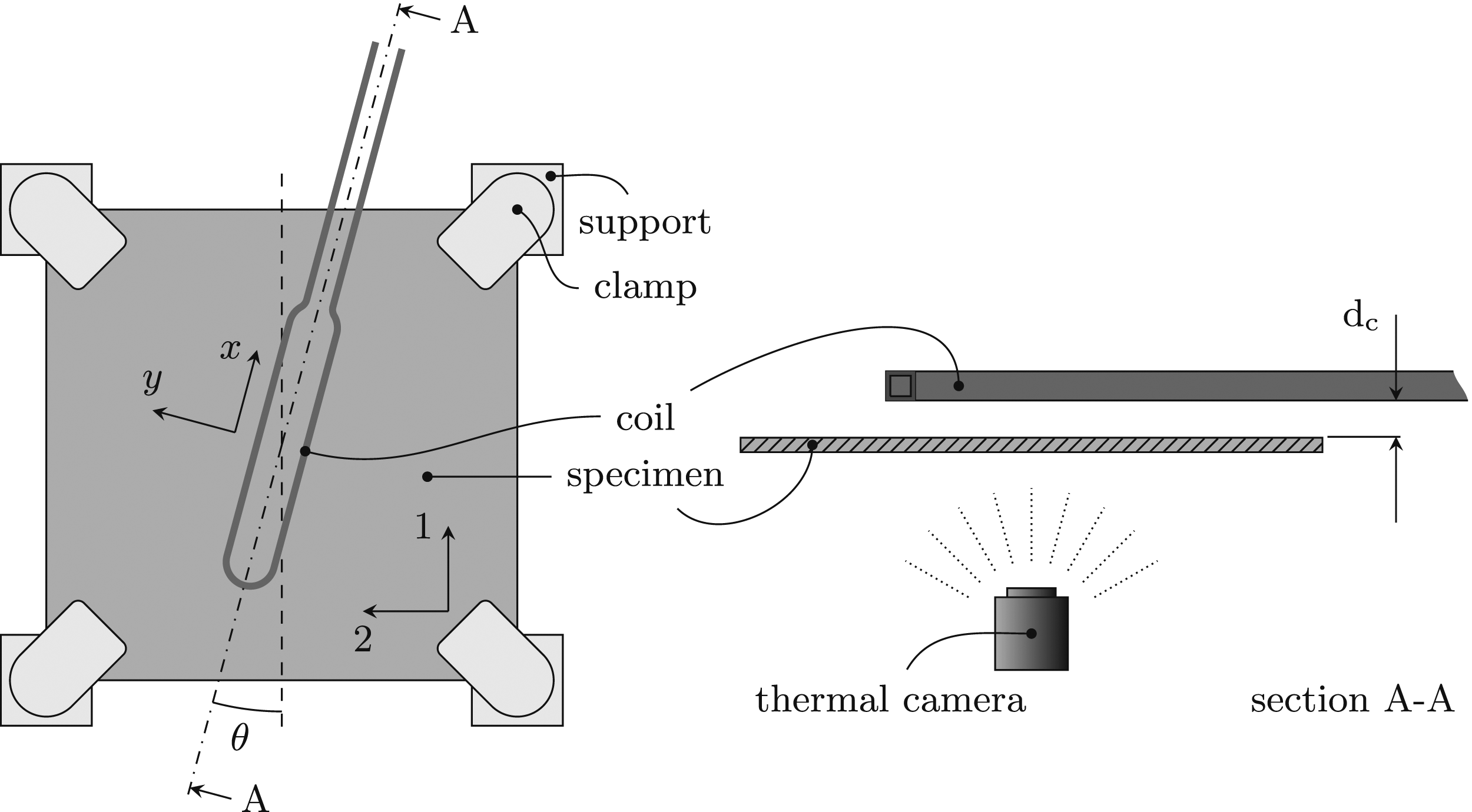

In order to ensure that only induction behaviour was observed and to reduce the influence of the heated material’s thermal behaviour, high heating rates were pursued to heat the specimen. Experiments were conducted at temperatures below the glass transition temperature in order to avoid any effects of phase changes and secondary transitions that may be associated with the material’s behaviour above this temperature. An Ambrel EASYHeat 8310 LI system was utilised, providing a 380 A root mean square current at 344.9 ± 0.5 kHz to heat the specimen for 1.00 ± 0.01 second, after which the current was switched off. Each measurement was repeated five times on one specimen.

Experiments were conducted on a TPC specimen with varying coil orientations (θ = 0°, 15°, …, 90°). A thermal camera (FLIR A65) was used to monitor the temperatures of the bottom surface of the heated specimen. These temperature measurements were compared for validation with E-type thermocouple measurements which are considered to be only weakly influenced by the electro-magnetic field. The thermocouple was fixed to the specimen by means of a tape at the center of the top and bottom surface of the specimen. The thermocouple measurements taken from the top and bottom surfaces of the laminate exhibited no discernible difference, which suggests that there is no significant heat generation gradient within the laminate layers. The coupling distance d_c between the specimen and the coil was 5 mm and fixed using a gauge block. The room temperature was measured prior to each individual heating experiment, values are provided in Table 1.

Table 1.

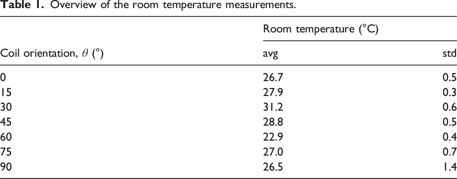
Overview of the room temperature measurements.

Coil orientation, θ (°)	Room temperature (°C)
Coil orientation, θ (°)	avg	std
0	26.7	0.5
15	27.9	0.3
30	31.2	0.6
45	28.8	0.5
60	22.9	0.4
75	27.0	0.7
90	26.5	1.4

The specimen was manufactured from a carbon fabric reinforced PolyEtherKetoneKetone (C/PEKK) prepreg fabric material (TC1320,¹⁷), supplied by Toray Advanced Composites (Nijverdal, the Netherlands) which consisted of T300JB carbon fibre bundles woven into a balanced five harness satin weave pattern, see Table 2, and stacked into a [(0/90)]_4s lay-up and consolidated, see Table 3, in a press (Pinette PEI, Chalon-sur-Saône, FR) using a steel (1.2311) picture frame. One fabric ply is denoted as (0/90), therefore [(0/90)]_4s lay-up refers to a cross-ply laminate with eight layers of fabric plies stacked symmetrically.

Table 2.

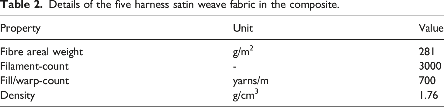
Details of the five harness satin weave fabric in the composite.

Property	Unit	Value
Fibre areal weight	g/m²	281
Filament-count	-	3000
Fill/warp-count	yarns/m	700
Density	g/cm³	1.76

Table 3.

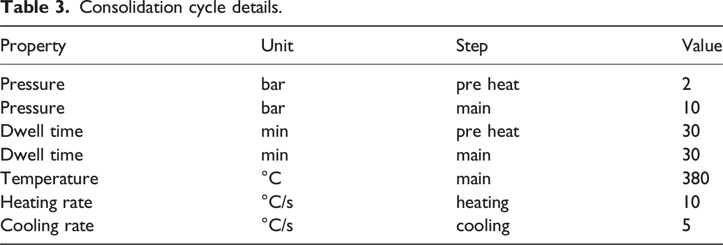
Consolidation cycle details.

Property	Unit	Step	Value
Pressure	bar	pre heat	2
Pressure	bar	main	10
Dwell time	min	pre heat	30
Dwell time	min	main	30
Temperature	°C	main	380
Heating rate	°C/s	heating	10
Cooling rate	°C/s	cooling	5

C-scan inspection did not reveal any defects. The specimen was cut by CNC contouring to 285 × 285 mm². The thickness t of the specimen was measured at nine evenly distributed positions over the specimen’s surface by micrometer prior to the induction heating experiments.

Since the findings of the induction heating experiments were extensively discussed in Ref. 7, these will only be used to validate the simulation results obtained in this study. Therefore, the test results are presented alongside the relevant simulation results, which are the focus of the present study.

Model set-up

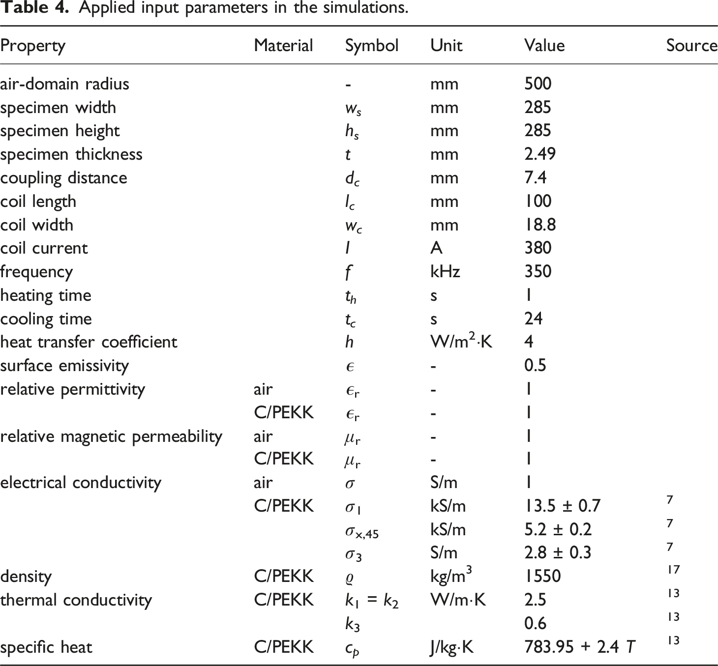
The approach employed in the simulations can be summarised as follows. A Comsol Multiphysics^®18 model was set-up to simulate the induction heating experiments. In the simulations, the Magnetic Fields (mf) module was utilised to solve the electromagnetic problem in the frequency domain, thereby calculating the Joule heating. The Heat Transfer in solids (ht) module was then employed to solve a transient thermal model, with the Joule heating determined from the mf-module as the heat source. This section discusses the equations being solved and the setup of the Finite Element (FE) model, including its applied input parameters outlined in Table 4.

Table 4.

Applied input parameters in the simulations.

Property	Material	Symbol	Unit	Value	Source
air-domain radius		-	mm	500
specimen width		w _s	mm	285
specimen height		h _s	mm	285
specimen thickness		t	mm	2.49
coupling distance		d _c	mm	7.4
coil length		l _c	mm	100
coil width		w _c	mm	18.8
coil current		I	A	380
frequency		f	kHz	350
heating time		t _h	s	1
cooling time		t _c	s	24
heat transfer coefficient		h	W/m²⋅K	4
surface emissivity		ϵ	-	0.5
relative permittivity	air	ϵ _r	-	1
	C/PEKK	ϵ _r	-	1
relative magnetic permeability	air	μ _r	-	1
	C/PEKK	μ _r	-	1
electrical conductivity	air	σ	S/m	1
	C/PEKK	σ ₁	kS/m	13.5 ± 0.7	⁷
		σ _x, ₄₅	kS/m	5.2 ± 0.2	⁷
		σ ₃	S/m	2.8 ± 0.3	⁷
density	C/PEKK	ϱ	kg/m³	1550	¹⁷
thermal conductivity	C/PEKK	k₁ = k₂	W/m⋅K	2.5	¹³
		k ₃		0.6	¹³
specific heat	C/PEKK	c _p	J/kg⋅K	783.95 + 2.4 T	¹³

Equations

The electromagnetic analysis is performed by solving Maxwell’s equations which are a set of equations governing the interrelations between the fundamental electromagnetic quantities. These are expressed here in differential form as it is applicable to the finite element method for solving time-varying fields.

\nabla \times H = J + \frac{\partial D}{\partial t},

(2a)

\nabla \times E = - \frac{\partial B}{\partial t},

(2b)

\nabla \cdot D = ϱ_{e},

(2c)

\nabla \cdot B = 0 .

(2d)

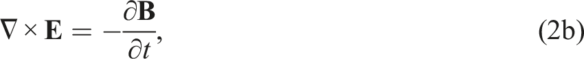
In this set of equations, the time is denoted by t, the electric field intensity by 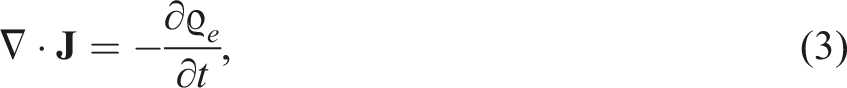E, the electric flux density by D, the magnetic field intensity by H, the magnetic flux density by B, the current density by J and the electric charge density by ϱ_e. Equations 2a and b are commonly known as Maxwell-Ampère’s law and Faraday’s law, respectively. Equations 2c and d can be regarded as two different forms of Gauss’ law, namely the electric and magnetic forms, respectively. These Maxwell’s equations are complemented with the fundamental continuity equation

\nabla \cdot J = - \frac{\partial ϱ_{e}}{\partial t},

(3)

and supplemented by appropriate constitutive relations depending on the nature of the media; for linear media:

D = ϵ_{0} E + P,

(4a)

B = μ_{0} (H + M),

(4b)

J = σ E,

(4c)

where ϵ₀ is the permittivity of vacuum, μ₀ is the permeability of vacuum, and σ is the anisotropic electrical conductivity. The electric polarization vector P characterises the polarisation of the material in response to an applied electric field E, and the magnetisation vector M similarly quantifies the magnetisation of the material when a magnetic field H is imposed.

The transient temperature distribution T in the specimen is calculated, applying the obtained current density J, in

ϱ c_{p} \cdot \frac{\partial T}{\partial t} = \nabla T \cdot k \cdot \nabla T + J \cdot E,

(5)

where c_p denotes the specific heat capacity of the heated material, ϱ its density and k the anisotropic thermal conductivity.

Implementation of the electrical conductivity

In Ref. 7, the electrical conductivity of a TPC material, reinforced with a balanced fabric was measured. It was demonstrated that the apparent electrical conductivity can be approximated according to

σ_{x, θ} = σ_{1} - (σ_{1} - σ_{x, 45}) | \sin 2 θ |,

(6)

where the in-plane direction is denoted by x, and θ is the angle between the material’s first principal direction and the direction of the electrical field E. The orientation angle θ is intentionally employed to represent both the fabric’s direction in the electrical conductivity measurements and the coil’s orientation, as the latter was the direction along which eddy currents predominantly flowed in the fabric during the induction heating experiments. This aligns with the conventions adopted in Ref. 7. It is important to acknowledge that the coordinate systems for the coil and the material remain independent.

This implies that σ_{x, 0} = σ₁, which is the measured electrical conductivity in the fabric’s warp direction. Similarly, for the material’s transverse direction, the measured electrical conductivity was σ_{x, 90} = σ₂. Considering that the material was reinforced with a balanced carbon fabric, it is assumed that σ₂ = σ₁. This approach has the advantage of only requiring direct current measurements to determine σ1 and σ_{x, 45} to approximate the anisotropic electrical conductivity. As demonstrated in Ref. 7, the conductivity in the laminate’s normal direction σ_{z, θ} is not dependent on the in-plane direction of the electrical field, hence σ_{z, θ} = σ₃.

Consequently, in Comsol Multiphysics^®18, a user-defined planar isotropic electrical conductivity can be assigned to the laminate domain, which is presented as a 3 × 3 matrix with σ_{x, θ} (Equation (6)) at the first two principal directions and σ₃ at the third principal direction. The 3 × 3 conductivity matrix in Comsol Multiphysics^®18 used in the presented simulations is as follows: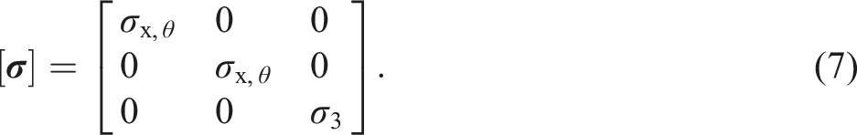

[σ] = [\begin{array}{l} σ_{x, θ} & 0 & 0 \\ 0 & σ_{x, θ} & 0 \\ 0 & 0 & σ_{3} \end{array}] .

(7)

The in-plane direction θ of 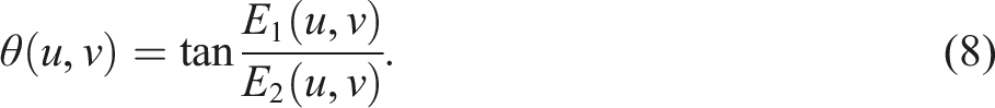E in the laminate domain, applied in equation (6), is defined using the direction of the electric field E with respect to the local coordinate system of the ply, E varies throughout the domain. In the FE model, the angle θ at the in-plane where position (u, v) was determined by:

θ (u, v) = \tan \frac{E_{1} (u, v)}{E_{2} (u, v)} .

(8)

This method leads to a heterogeneous electrical conductivity in the laminate domain. Therefore, this electrical conductivity definition is denoted as a function of the orientation of the electric field strength in the remainder of the text.

The applied electrical conductivity in equations (2) and (4) depends on the direction of the electrical field and vice versa. Therefore, equations (2)–(4) are iteratively solved according the iteration scheme for E shown in Figure 3, in which the convergence criterion is met when either the relative error in the solution vector or the relative error in the residual vector is less than the relative tolerance. As described in more detail in the Comsol Multiphysics^®18 reference manual, the relative error is computed as the weighted Euclidean norm of the error or residual vector, where the weights are based on the magnitude of the solution or residual vector and a factor that is used to account for the non-linearity of the problem.

Figure 3.

Schematic visualisation of the iterative process to obtain the solution of the electro-magnetic fields, represented by 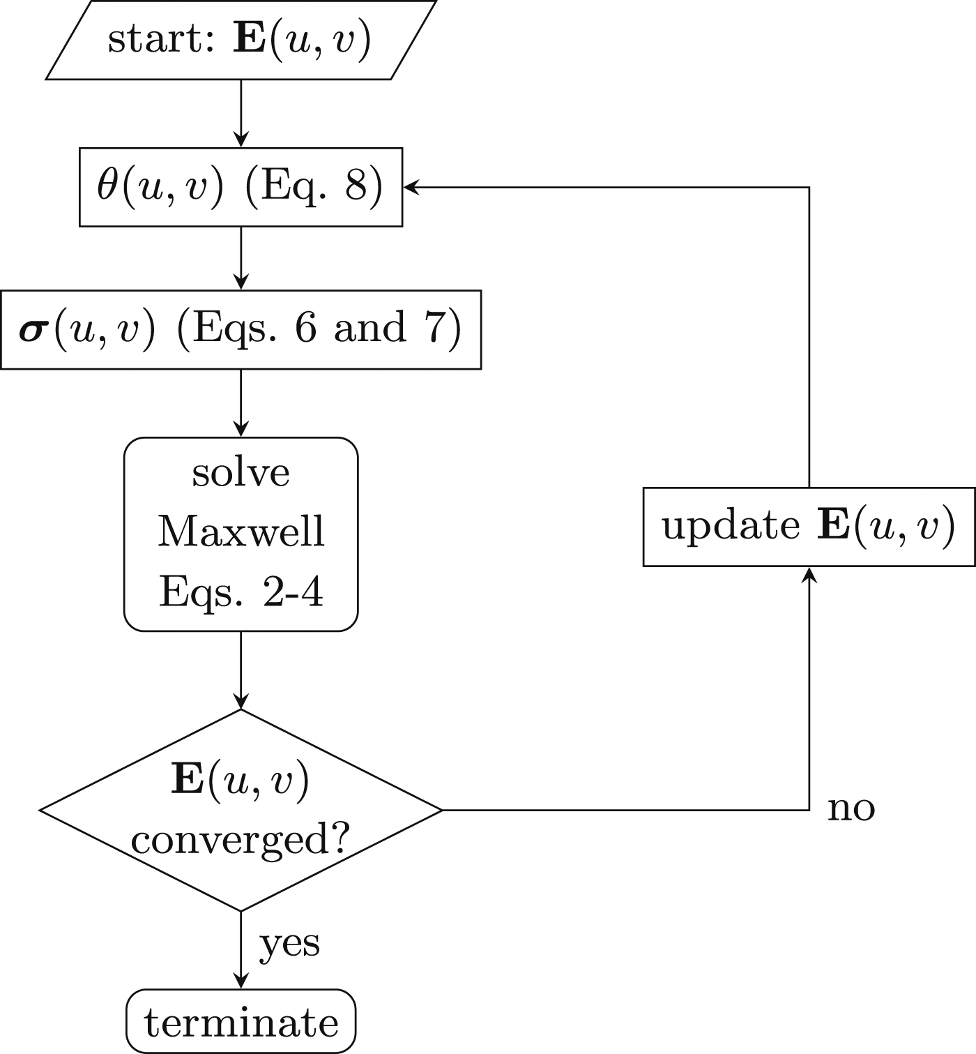E.

Material properties

The material parameters in the simulation model comprise the electromagnetic properties of the specimen and the ’air’ domain, see equation (4), as well as the thermal material properties of the specimen domain, equation (5).

The anisotropic electrical conductivity properties of the heated C/PEKK material measured in7 were used in the present model, these are provided in Table 4. Measurements of the electrical conductivity of the C/PEKK material at elevated temperatures did not demonstrate a significant variation for temperatures between room temperature and 150°C, which is just below the glass transition temperature of this material. Therefore, an temperature independent electrical conductivity was used in the simulations. An electrical conductivity of 1 S/m was applied to the ’air’ domain to avoid a poorly-conditioned problem and thus circumvent numerical instabilities. Alternatively, damping may be applied.

Previous studies have demonstrated that dielectric heating does not occur at the given experimental conditions.^7,19 It is likely that dielectric heating may occur at frequencies of the order of MHz; however, the set-up utilised was not capable of operating at these frequency ranges. Consequently, dielectric heating is not considered and a relative permittivity ɛ_r = 1 is applied. Furthermore, as the air and specimen materials are both non-magnetic, the relative magnetic permeability μ_r = 1 is set for both materials.

The thermal properties of C/PPS¹³ were employed for the C/PEKK material due to the similarity of their respective constituents and fibre volume fraction. The employed specific heat c_p, thermal conductivity k and density ϱ values are provided in Table 4.

Geometry and discretisation

The FE model to calculate the electromagnetic field comprised the laminate, the coil and the surrounding air-domain. The dimensions of the heated specimen and the hairpin coil, shown in Figures 1 and 2, are detailed in Table 4. The air-domain was modelled as a sphere with a radius of 500 mm, centred at the central position of the specimen’s top surface.

The laminate and air-domains were meshed using tetrahedral elements, and the coil was meshed using line elements. Quadratic discretisation was applied to describe the electromagnetic and temperature fields. The element size for the outer surfaces of the air-domain was set to 25 mm. The mesh size increased steadily from the fine mesh of the laminate and coil to the coarse mesh of the external surface of the air-domain. In order to provide an indication of the total geometry in the FE model, Figure 4(a) presents the full mesh of the model, in this example consisting of 195k elements, omitting a quarter of the air domain for the purpose of showing the mesh of the air domain in comparison to the mesh of the laminate. Figure 4(b) only shows the mesh of the coil and the laminate.

Figure 4.

Mesh details of the coil and the laminate; (a) overall impression of the mesh; (b) overview of the laminate and the coil; (c) detailed top view of the straight section of the coil above the laminate; (d) a single element in the thickness direction of the laminate domain.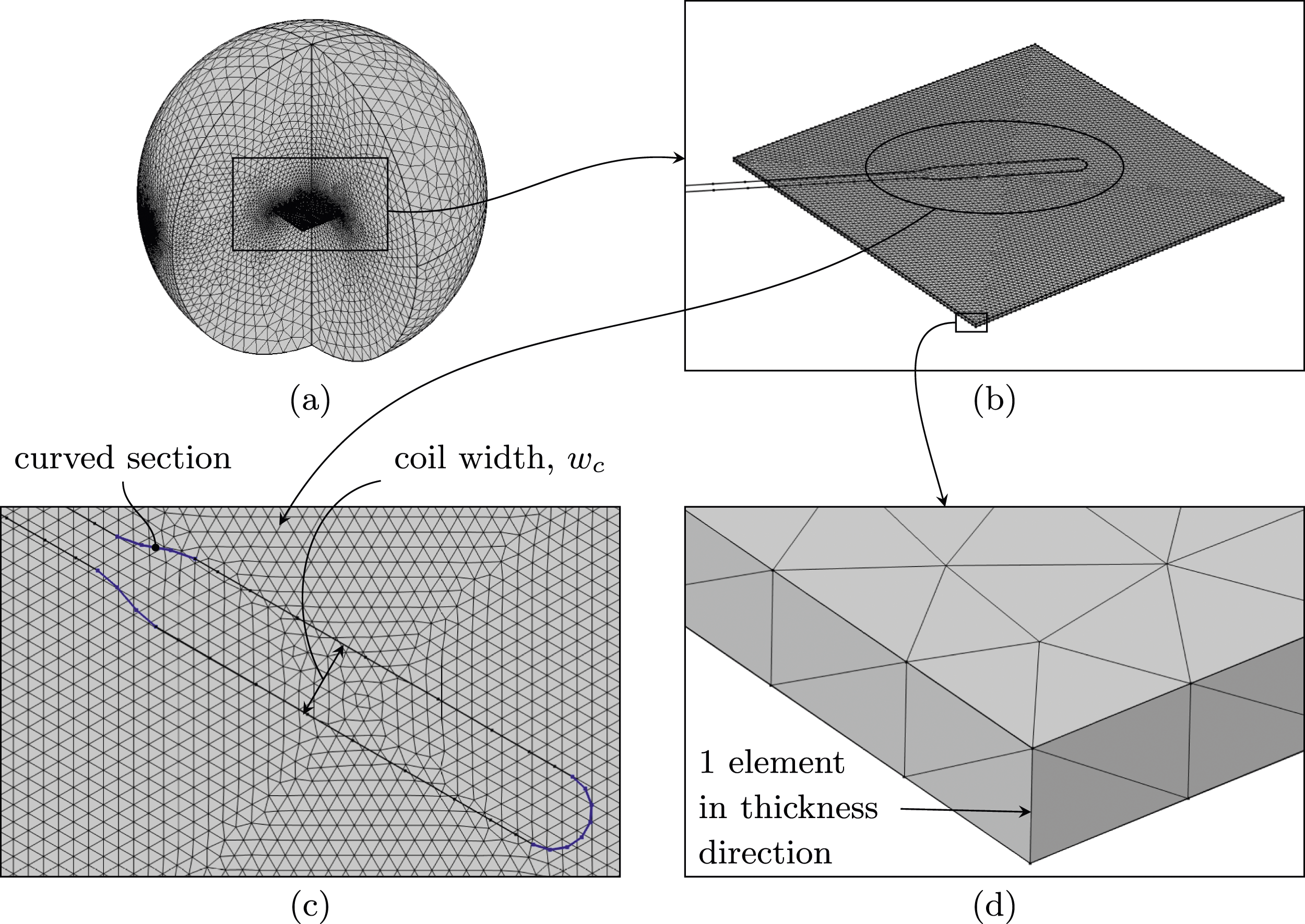

A mesh convergence study resulted in a maximum element size of 5 mm for the curved sections in the coil, as illustrated in Figure 4(c). A minimum of five elements along the coil width, w_c, in the laminate domain was applied in order to describe the temperature gradient between the coil’s two straight sections. Subsequently, the maximum element size for the laminate domain in the model was set to a value of 18.8/5 ≈ 3.8 mm. The limited temperature gradient in the thickness direction, due to the experimental conditions, was described by a single quadratic element in specimen’s thickness direction, see Figure 4(d) for a detailed view of the specimen’s mesh which was applied for both the electro-magnetic as well as the thermal analysis.

Loads and boundary conditions

In order to calculate the electric field, a root mean square current of I = 380A was applied as an edge current to the coil in the FE model at a frequency f of 350 kHz, which was in line with the electromagnetic load during the experiments. Furthermore, a homogeneous Dirichlet boundary condition was imposed at the outer boundary of the simulation domain, such that the magnetic vector potential was equal to zero.

Joule heating, derived from the electromagnetic problem, was applied in the heating step for one second, which was consistent with the heating time in the experiments. The thermal model comprised solely the specimen; hence, convective and radiation boundary conditions were defined to simulate the surrounding air. The heat transfer coefficient, h, for natural convection (for air, typically h = 4-12 W/m²⋅K) or forced convection (for air, h > 12 W/m²⋅K) was set to 4 W/m²⋅K for all the outer surfaces of the laminate to consider the natural convection of air. The emissivity, ϵ, of a surface, which is an optical characteristic of the surface and ranges between 0 for white bodies and 1 for black bodies, regulates radiation. A basic sensitivity analysis showed that the radiation boundary condition had a negligible effect on the temperature predictions and could thus be disregarded. Nonetheless, it was applied with ϵ = 0.5 for the sake of completeness. The specimen’s initial temperature and the ambient temperature for both the convective and radiation boundary conditions were set to the measured room temperatures for each individual experiment as provided in Table 1.

Validation models

The simulation results using the heterogeneous isotropic electrical conductivity model were compared to the results obtained from simulations using the planar uniform isotropic and the uniform anisotropic electrical conductivity models, in order to assess the efficacy of the presented electrical conductivity definition. Except for the electrical conductivity model applied, the validation models were identical to the model already described. Assuming a balanced material, the in-plane electrical conductivity for both definition types was σ₂ = σ₁.

The planar uniform isotropic electrical conductivity was assigned according to equation (6) with σ_x, _θ = σ₁ with the material’s directions in agreement with the coordinate system shown in Figure 1.

The uniform anisotropic electrical conductivity was assigned to the specimen according to the descriptions in Refs. 5,6; this method resulted in modelling each virtual UD-layer in the laminate separately using the virtual uni-directional (UD) properties σ₁, σ₂ and σ₃. The electrical conductivity was assigned similarly to the planar uniform isotropic model, however the virtual UD-layers representing the electrical conductivity in the material’s first principal direction were assigned an σ₁ ≠ 0 and σ₂ = 0 while the layers representing the electrical conductivity in the material’s second principal direction were assigned an σ₁ = 0 and σ₂ ≠ 0 with the material’s directions in agreement with the coordinate system shown in Figure 1.

The UD-layer defining the electrical conductivity in the material’s first principal direction was placed at the bottom of the ply in line with the coordinate system shown in Figure 1, and the top layer of each ply thus represented the electrical conductivity in the second principal direction. Figure 5 shows a detail of the mesh and the described electrical conductivity assignment in accordance with the detail as depicted in Figure 4(d). The uniform anisotropic electrical conductivity model in this study resulted in a mesh of the specimen, consisting of eight plies, consisting of 16 virtual stacked element layers over the thickness. The remaining meshing settings in the uniform anisotropic model remained unchanged.

Figure 5.

Detail of the specimen’s mesh in the uniform anisotropic model. Additionally, the UD-layer electrical conductivity assignment is depicted.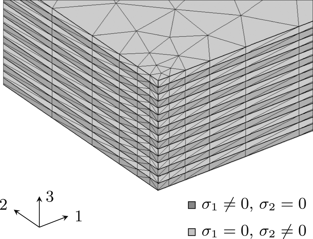

In agreement with the heterogeneous isotropic electrical conductivity model, the electrical conductivity in the material’s third principal direction, σ₃, was assigned the measured σ₃ of 2.8 kS/m as provided in Table 4.

Simulation results

This section presents the outcome of the simulations conducted. The simulations were executed on a DELL laptop equipped with an Intel^® Core^TM i7-8750H CPU at 2.20 GHz, with 16.0 GB random-access memory.

Firstly, the solution times for the electro-magnetic simulations are provided in Table 5 alongside the degrees of freedom (DOF) the simulations were solved for for all models. As the heterogeneous isotropic electrical conductivity model results in a non-linear problem which is solved iteratively with a straightforward Picard iteration updating the conductivities in each element at the end of each iteration according to the local electric field prediction, see Figure 3, the required iterations are provided for the non-linear solver. Secondly, a qualitative judgement is made with regard to the temperature distribution and, lastly, a more quantitative evaluation is conducted by examining the heating rates.

Table 5.

Overview of the computation times for the different simulations.

θ (°)	Heterogeneous isotropic			Planar uniform isotropic		Uniform anisotropic
θ (°)	Time (s)	Iters [#]	DOF (M)	Time (s)	DOF (M)	Time (s)	DOF (M)
0	2136	13	1.2	84	1.2	4004	5.4
15	11,367	33	1.5	129	1.5	2960	5.2
30	1643	12	1.3	86	1.3	3647	5.4
45	1612	14	1.2	82	1.2	3167	5.2
60	1750	11	1.3	100	1.3	3665	5.4
75	10,814	31	1.5	120	1.5	3013	5.2
90	2136	13	1.2	97	1.2	3716	5.4

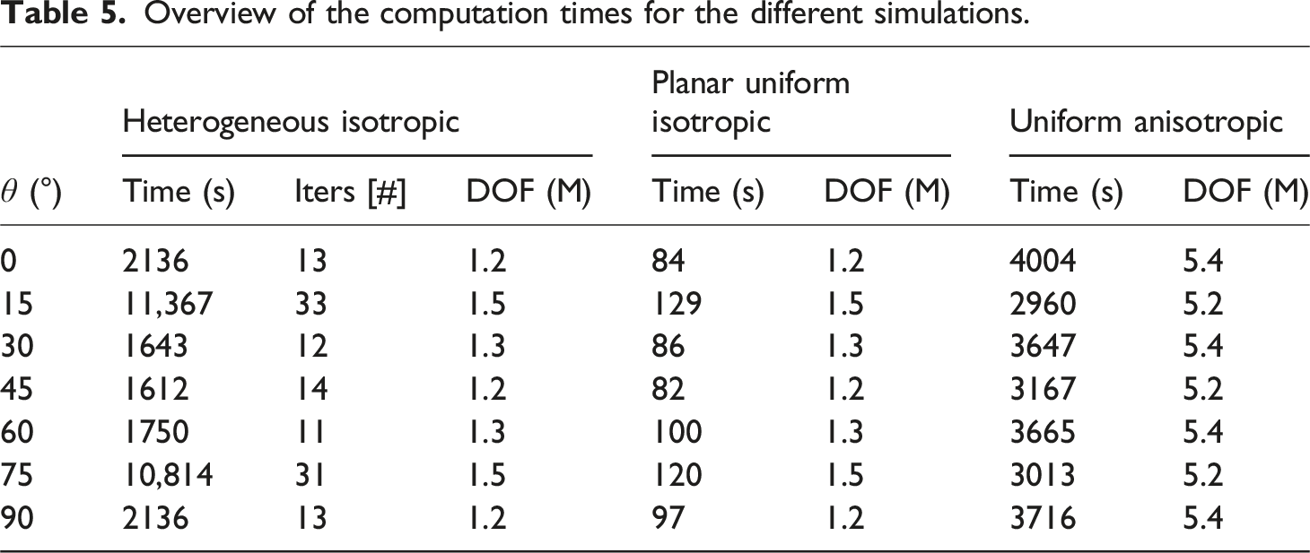
Computation times

Regardless of the predictive accuracy of the electrical field, Table 5 shows that the computation times for simulations using the heterogeneous isotropic electrical conductivity definition are considerably higher than those for simulations using the planar uniform isotropic electrical conductivity definition, and are roughly half of those required for simulations using the uniform anisotropic electrical conductivity definition. Exceptions were observed in the simulations when the coil orientation θ was 15° and 75°, where a larger number of iterations was required to reach a converged solution. The probable numerical cause of the slow convergence could be attributed to regions where the electric field is small, which may effectively have very large local directional fluctuations, leading to numerical instability.

Adjustments to the underlying non-linearity, iteration process, or convergence criterion could lead to faster convergence while maintaining accuracy. However, further research is needed to confirm this.

Apparent in-plane electrical conductivity fields

Despite the challenge of validating electromagnetic field predictions using experimental data, intermediate results are presented in this section and, where feasible, compared with corresponding simulation results from both the planar uniform isotropic and uniform anisotropic models.

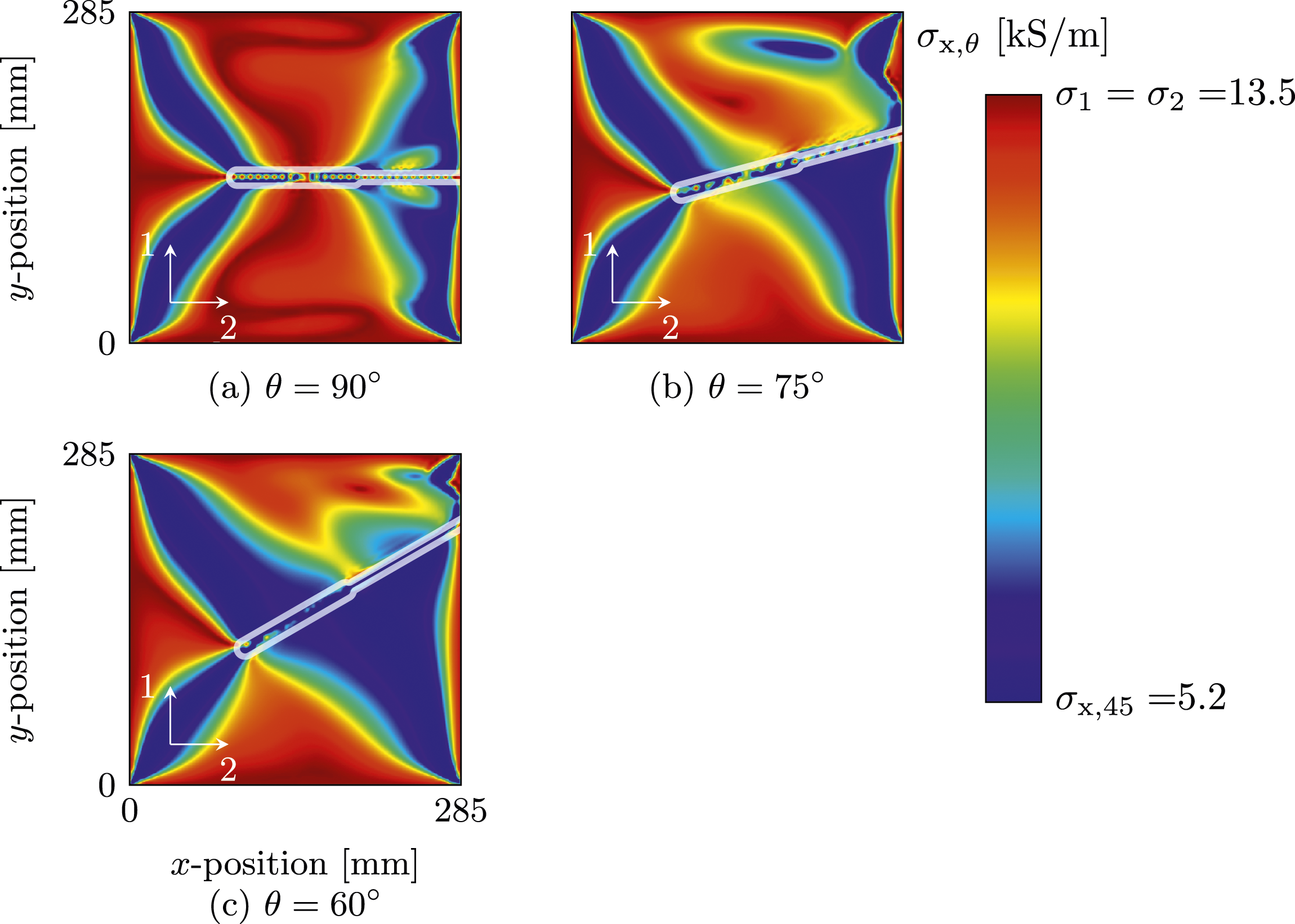
The novelty in the heterogeneous isotropic electrical conductivity definition approach, the applied apparent in-plane electrical conductivity, is demonstrated in Figure 6, which shows the distribution of σ_{x, θ} as a result of the predicted orientation of the electric field. The apparent in-plane electrical conductivity is symmetric around the coil’s length direction (line A-A in Figure 1) for θ = 0°, 45° and 90°; σ_{x, θ} is not symmetric around the coil’s length direction for the other coil orientations. The overviews for the other coil orientations are provided in the Appendix. For the sake of clarity, the coil is rendered transparent to provide an impression of its location and orientation relative to the obtained heterogeneous electrical conductivity field in the laminate.

Figure 6.

In-plane electrical conductivity distribution for coil orientations θ = 0°, 15°, 30° and 45°.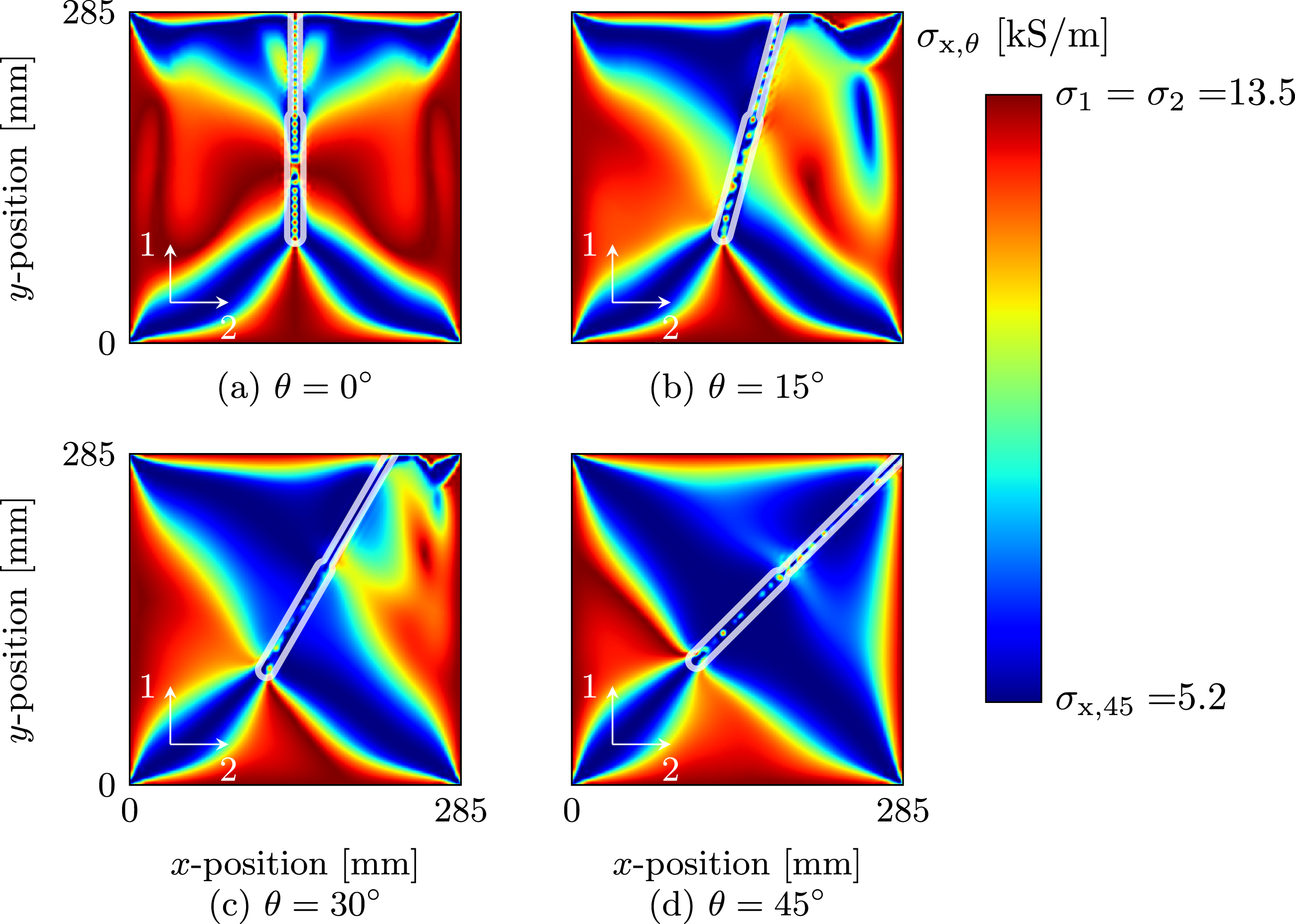

Figure 7 illustrates the predicted current density distributions at the bottom surface of the heated laminate for the three different methods. The electrical current density distributions in the sub-figures are grouped by electrical conductivity models (columns) and coil orientation θ (rows). Since the bottom surface was monitored by the thermal camera during the induction heating experiments, this surface was chosen to display the current density distribution.

Figure 7.

Current density distributions at the bottom surface of the specimen in the model for all coil orientations.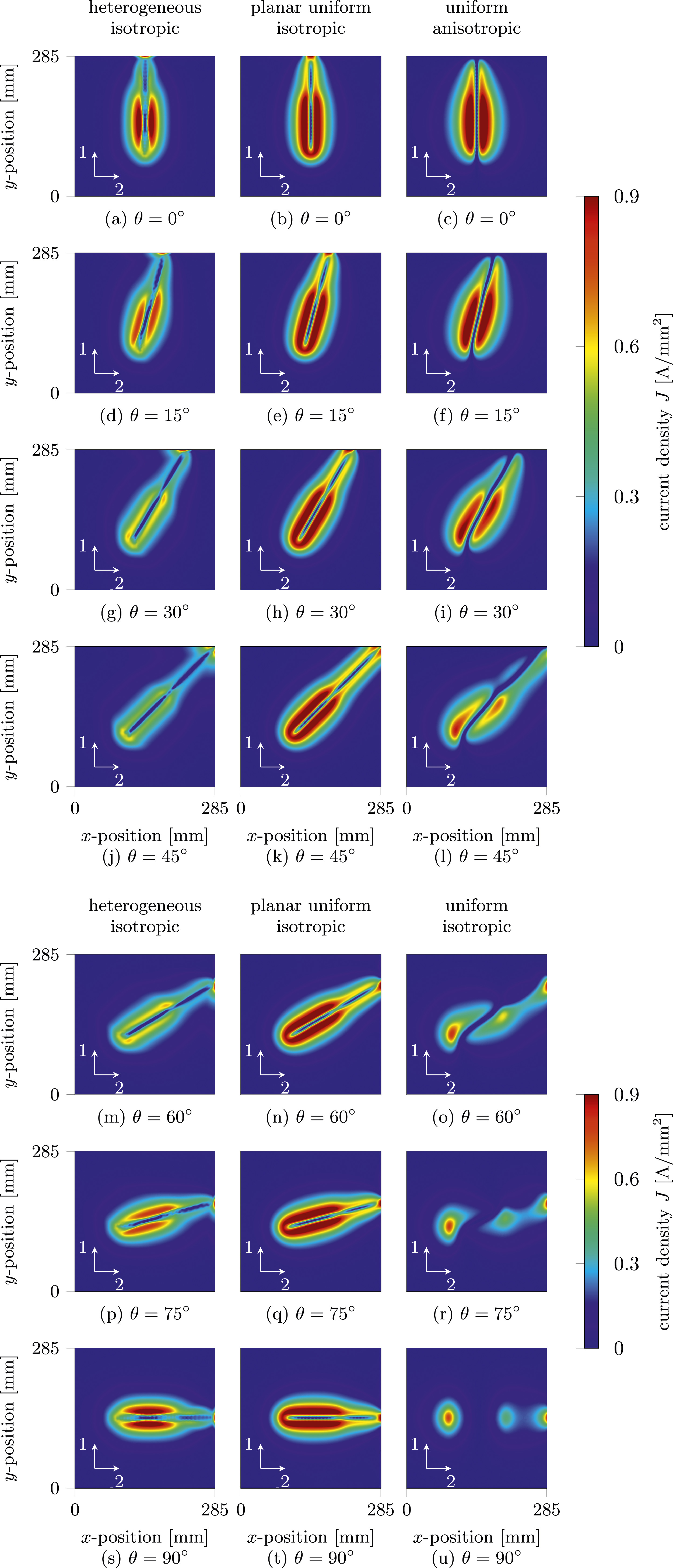

In Figure 7, it is evident that when employing the planar uniform isotropic electrical conductivity model, the effect of the coil orientation on the current density distribution is only minor, apart from an obvious rotation in the direction of θ. On the other hand, when using the two other models of the electrical conductivity, the magnitude, the shape and the rotation of the current density distributions are noticeably affected.

The current density distribution predicted by the heterogeneous isotropic and the planar uniform isotropic electrical conductivity models were found to have a high current density at the edge of the specimen beneath the coil. This high current density was not correspondingly predicted when using the uniform anisotropic model. It appeared that a high electrical current density at the bottom surface of the specimen was only predicted when the angle of the coil orientation matched that of the UD-layer at the bottom surface; namely, when θ > 45°.

Temperature distribution

The temperature distribution within the heated laminate was found to be dependent on the rotation of the induction coil, as demonstrated in Ref. 7. This is a consequence of the anisotropic electrical conductivity, resulting in the induced electric field varying for each coil orientation.

Figure 8 shows the measured temperature distribution for coil orientation θ = 45° after one second of heating at the specimen’s bottom surface. The thermocouple is highlighted in the figure.

Figure 8.

Measured temperature distribution at the bottom surface of the specimen at 1 sec. of heating for a coil orientation of θ = 45°.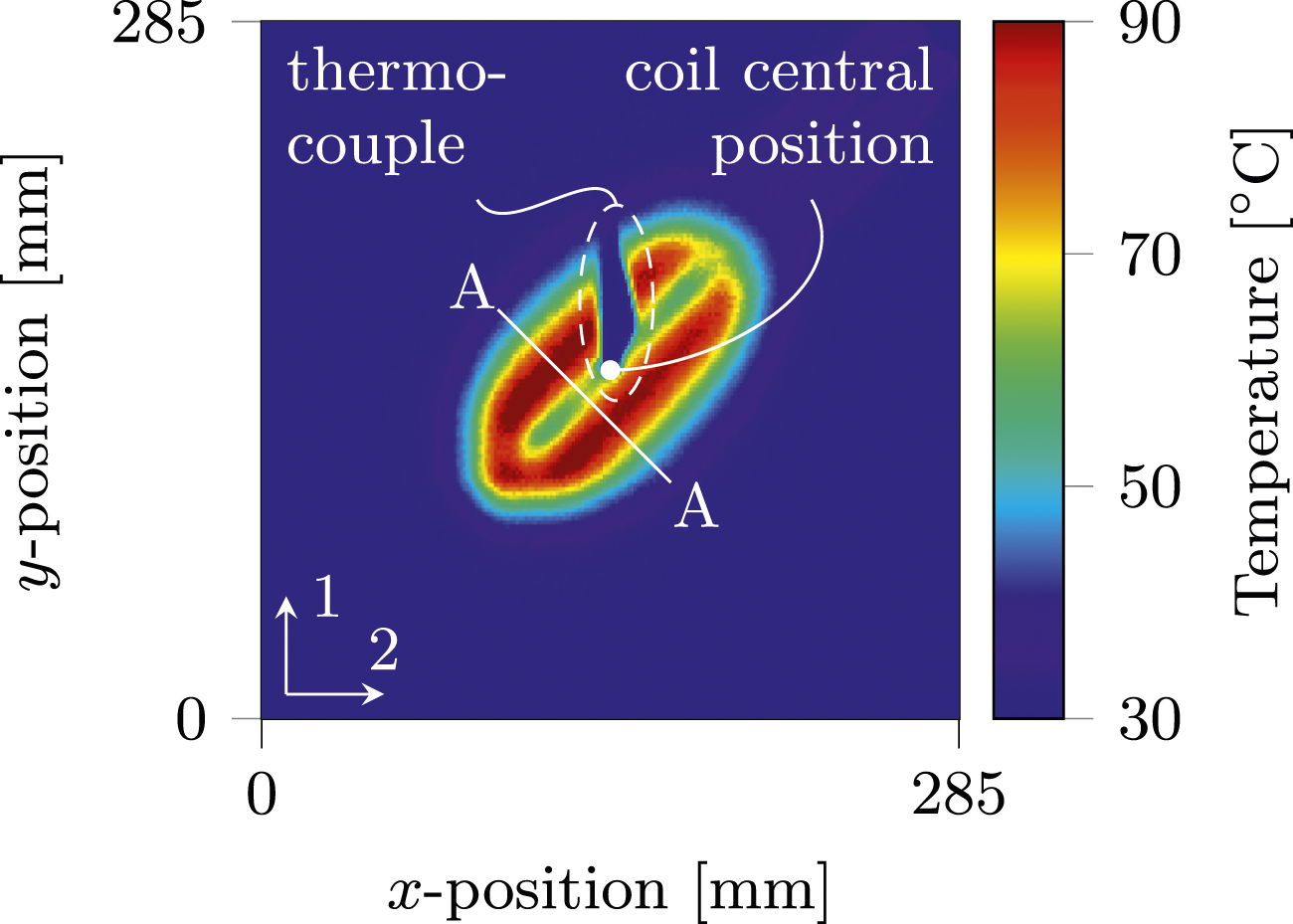

For evaluation purposes, temperature measurements along line A-A in Figure 8 were taken and compared with the simulation results. The cross-sections were slightly shifted from the central position of the coil to avoid the influence of the thermocouple tape on the measurements.

The predicted current density distributions, which were previously shown in Figure 7, were used to provide thermal loads that resulted in the specific heating patterns for each coil orientation. The predicted temperature distributions at the bottom surface of the specimen in the models, after one second of heating, are presented in Figures 9–15 alongside the measured temperature distribution at the same surface and heating time. Subfigure (a) shows the measured temperature distribution, while subfigures (b), (c), and (d) display the predicted temperature distributions according to the heterogeneous isotropic, planar uniform isotropic, and uniform anisotropic electrical conductivity models, respectively.

Figure 9.

Simulation validation for coil orientation θ = 0°: (a) experiment, (b) heterogeneous isotropic, (c) planar uniform isotropic, (d) uniform anisotropic.

Figure 10.

Simulation validation for coil orientation θ = 15°: (a) experiment, (b) heterogeneous isotropic, (c) planar uniform isotropic, (d) uniform anisotropic.

Figure 11.

Simulation validation for coil orientation θ = 30°: (a) experiment, (b) heterogeneous isotropic, (c) planar uniform isotropic, (d) uniform anisotropic.

Figure 12.

Simulation validation for coil orientation θ = 45°: (a) experiment, (b) heterogeneous isotropic, (c) planar uniform isotropic, (d) uniform anisotropic.

Figure 13.

Simulation validation for coil orientation θ = 60°: (a) experiment, (b) heterogeneous isotropic, (c) planar uniform isotropic, (d) uniform anisotropic.

Figure 14.

Simulation validation for coil orientation θ = 75°: (a) experiment, (b) heterogeneous isotropic, (c) planar uniform isotropic, (d) uniform anisotropic.

Figure 15.

Simulation validation for coil orientation θ = 90°: (a) experiment, (b) heterogeneous isotropic, (c) planar uniform isotropic, (d) uniform anisotropic.

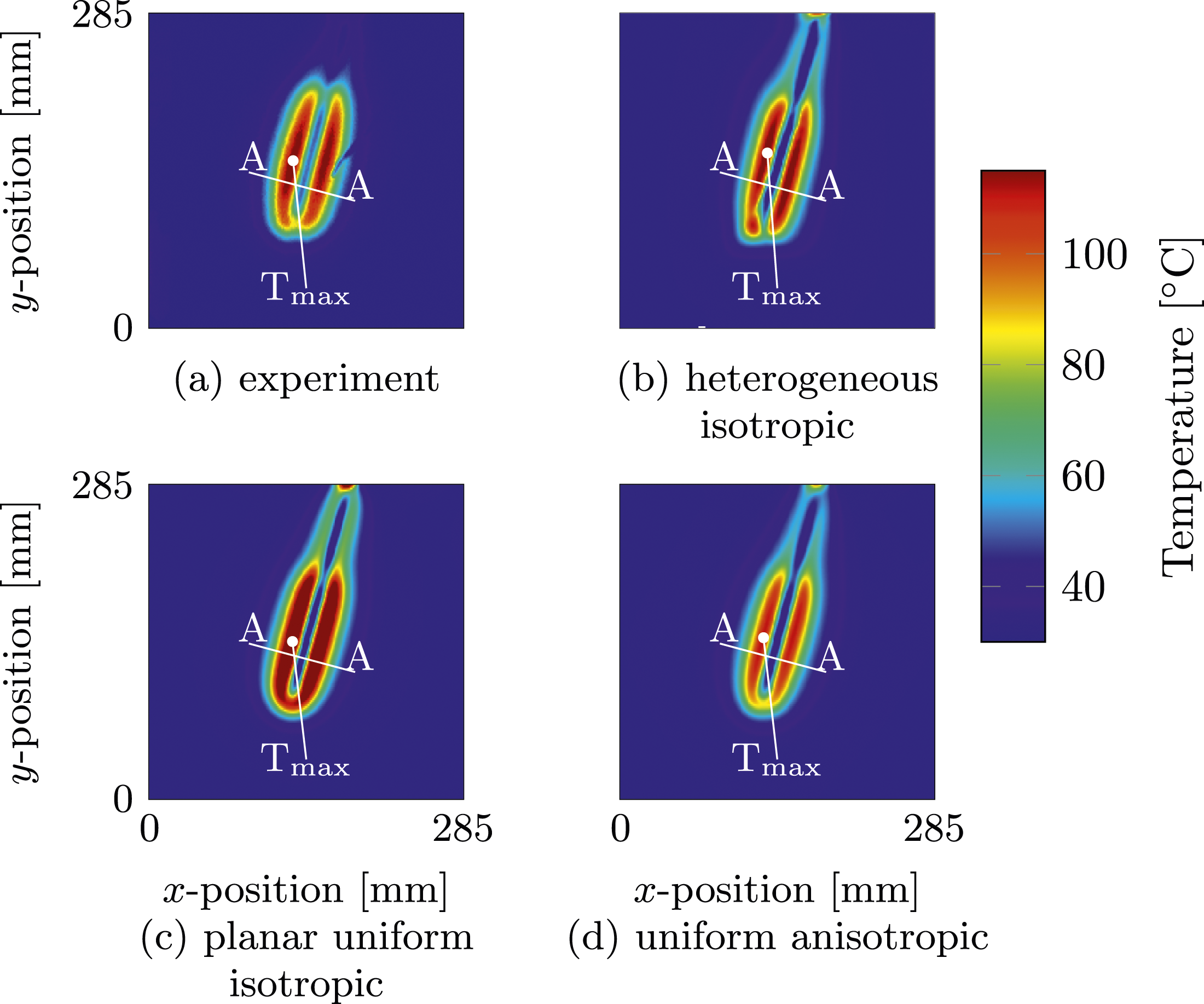
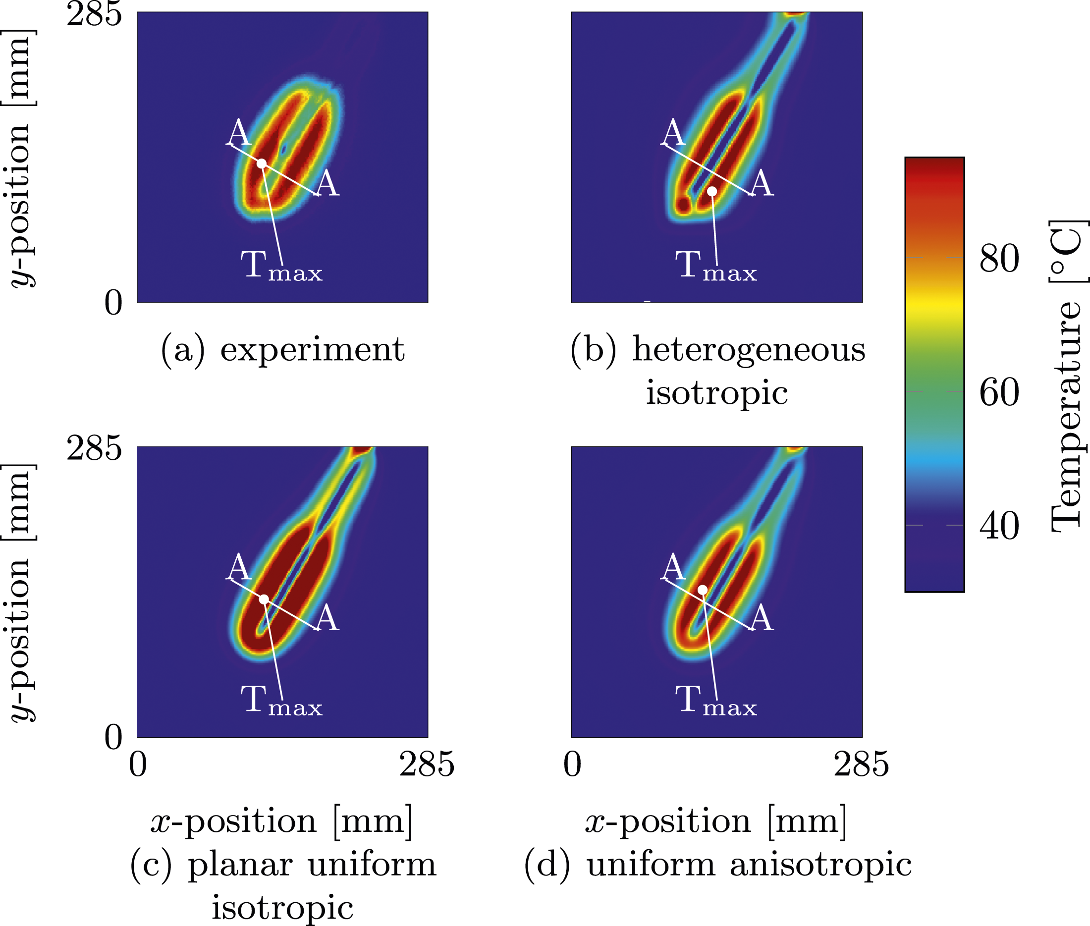
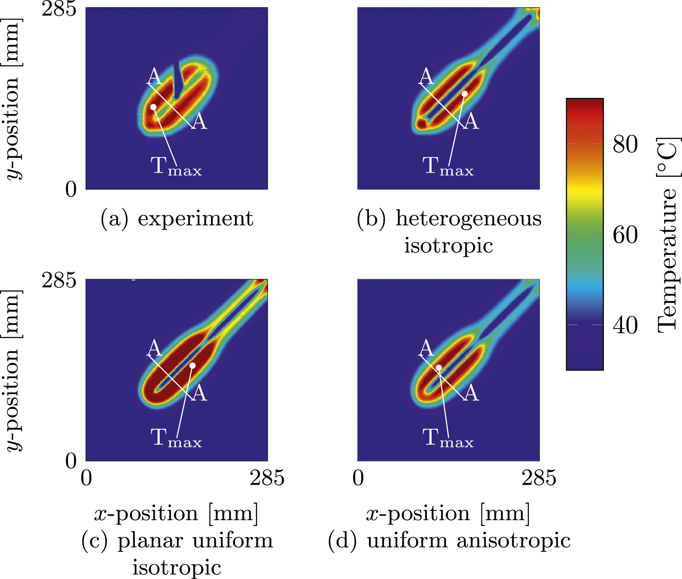
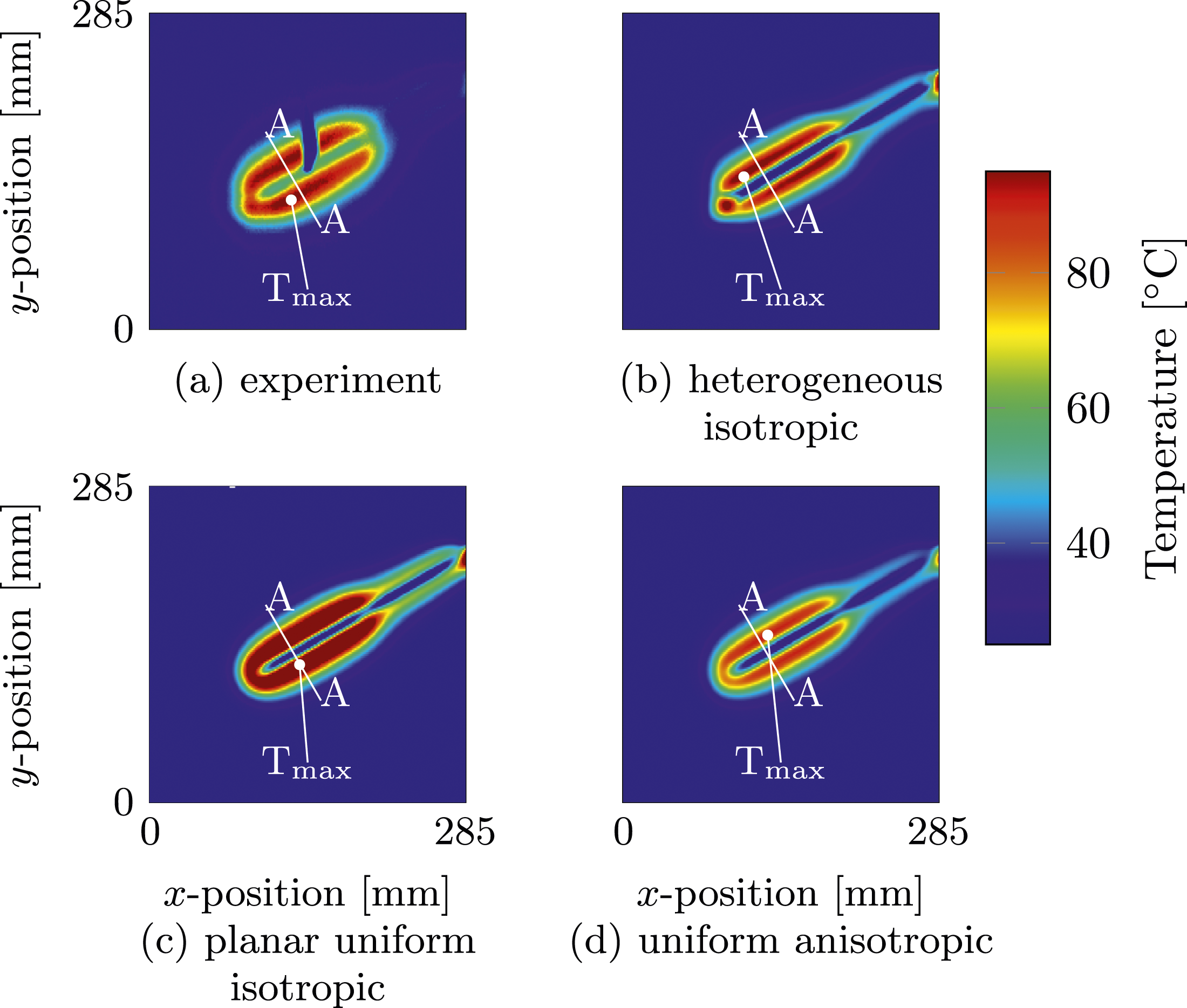
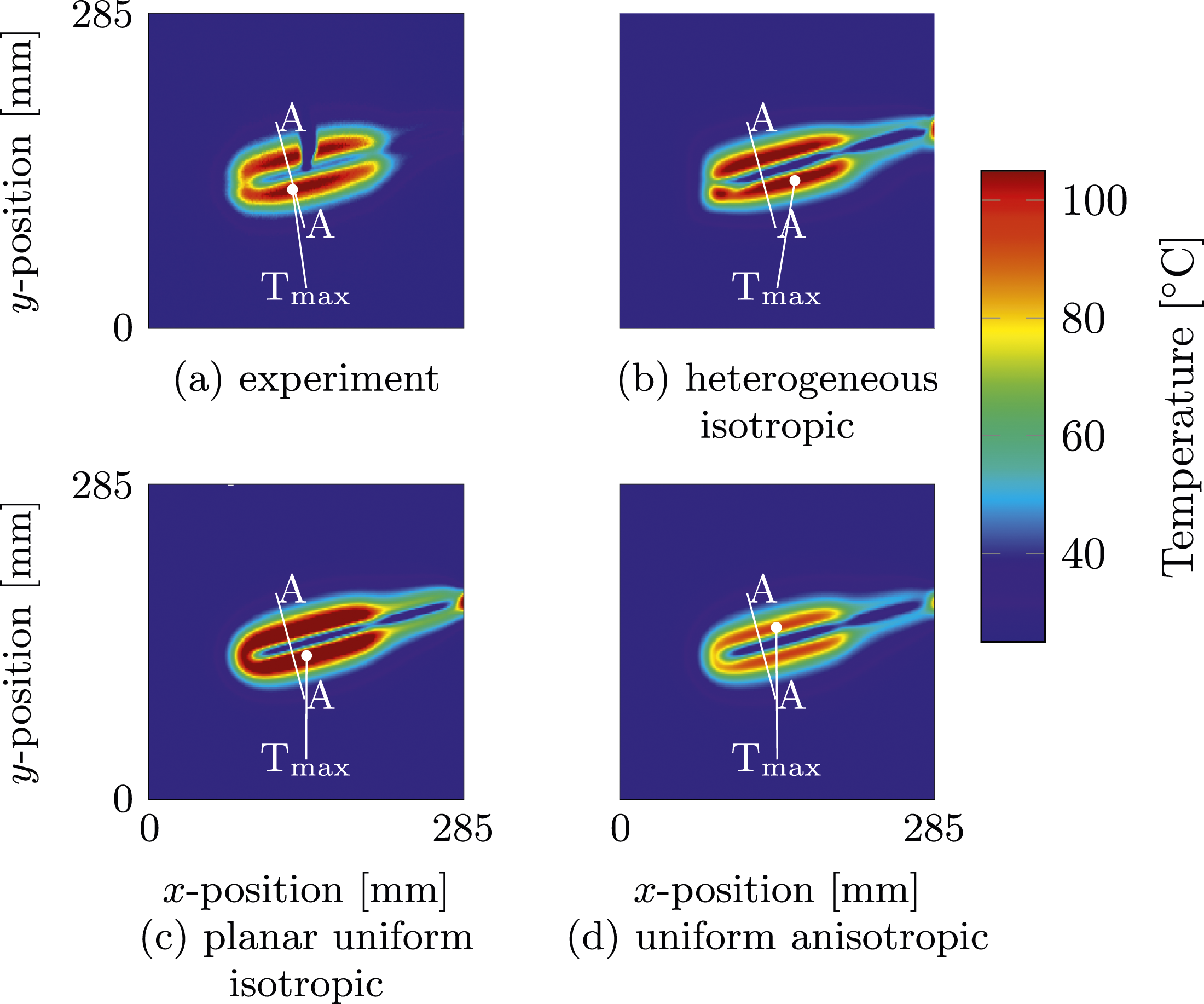
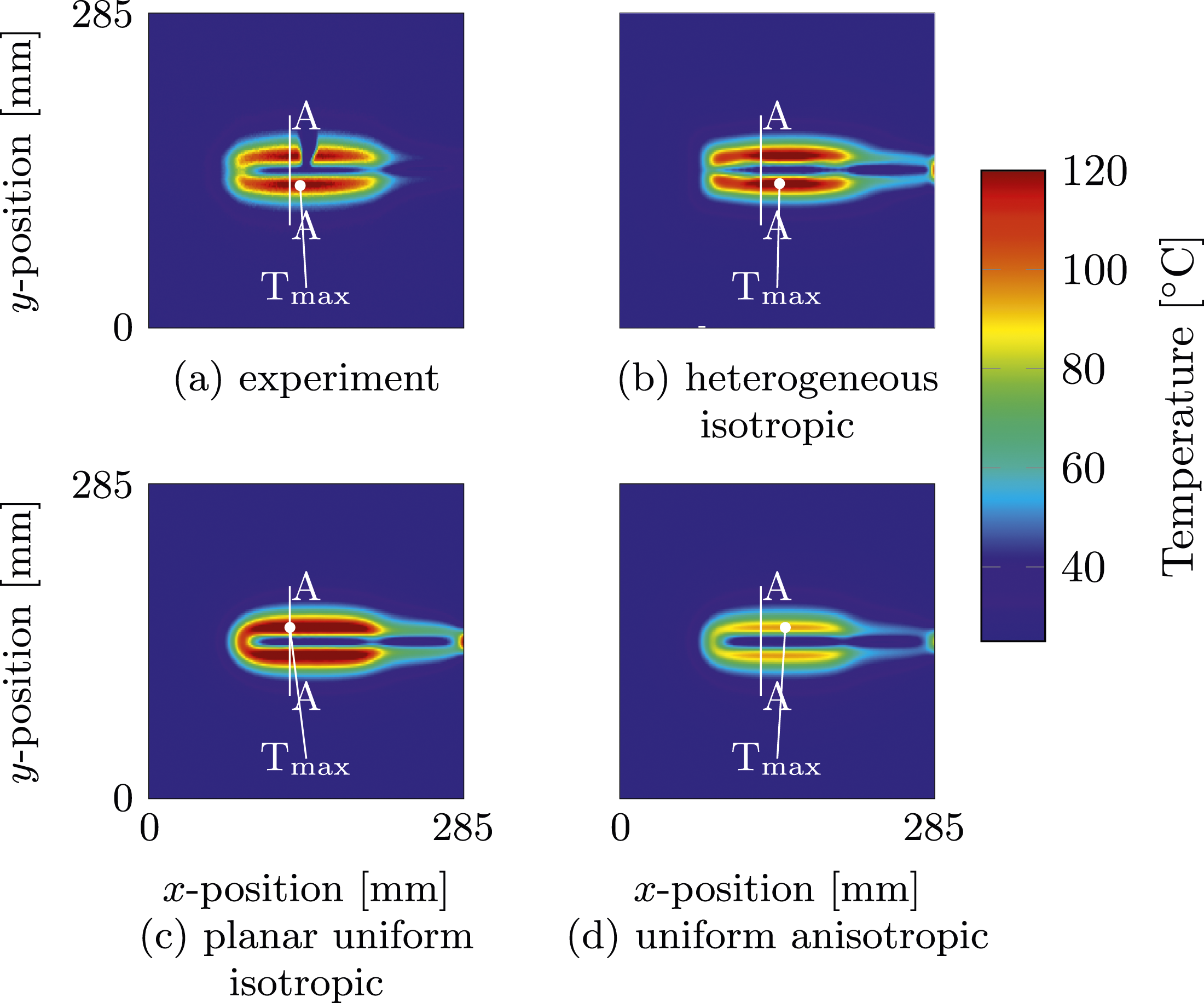
A comparison of the measured and predicted temperatures at the bottom surface of the specimen using the heterogeneous isotropic method to define the electrical conductivity, shows that the predictions largely correspond to the measured temperatures for all coil orientations.

The predicted temperature distributions for the planar uniform isotropic and uniform anisotropic electrical conductivity models largely agree with the temperature measurements for θ = 0° and 90°. However, for the remaining coil orientations, the predicted temperature distributions deviate from the measured temperature distributions. The temperature distribution predicted using the planar uniform isotropic electrical conductivity model appears to be a rotated version of the prediction at θ = 0°.

Utilising the planar uniform isotropic electrical conductivity model, temperatures are consistently overestimated for all coil orientations. Conversely, when employing the uniform anisotropic electrical conductivity model, temperatures are underestimated for all coil orientations, with the exception of θ = 45°. This is visualised utilising the data along the line A-A in Figures 9–15. The temperature profiles along A-A are provided in Figure 16.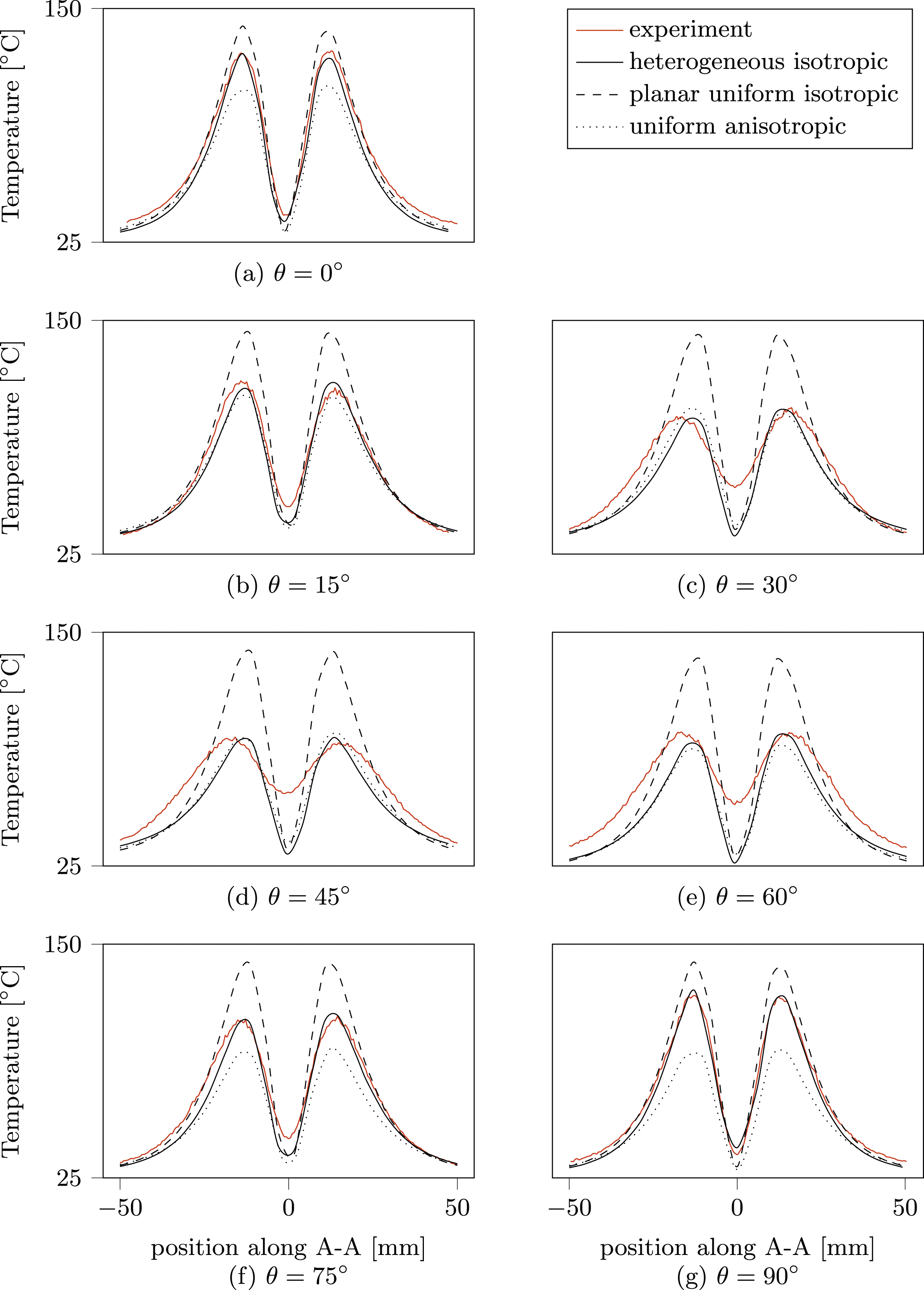

Figure 16.

Temperature profiles along A-A in Figures 9–15; predictions versus experiments.

It is evident from Figure 16 that the temperature profiles, predicted using the planar uniform isotropic electrical conductivity model, are equal for all coil orientations. The temperatures were underestimated using the uniform anisotropic model when the coil orientation approached or was aligned to the material’s first or second principal direction. Figure 16 indicates that the width of the predicted temperature profile along A-A is narrower than the width of the measured temperature profile across all models for 30° ≤ θ ≤ 60°.

Finally, the predicted and measured maximum temperatures at one second of heating and heating rates of the maximum temperature at the bottom surface of the laminate were compared. The heating rates were calculated from the T_max developments using values taken between 0.1 and 0.9 s, of which a representative overview for θ = 0° is provided in Figure 17.

Figure 17.

Development of the maximum temperature (T_max) over time for coil orientation θ = 0°, measurement and simulation results. The measurement data represents mean and standard deviation values of five measurements.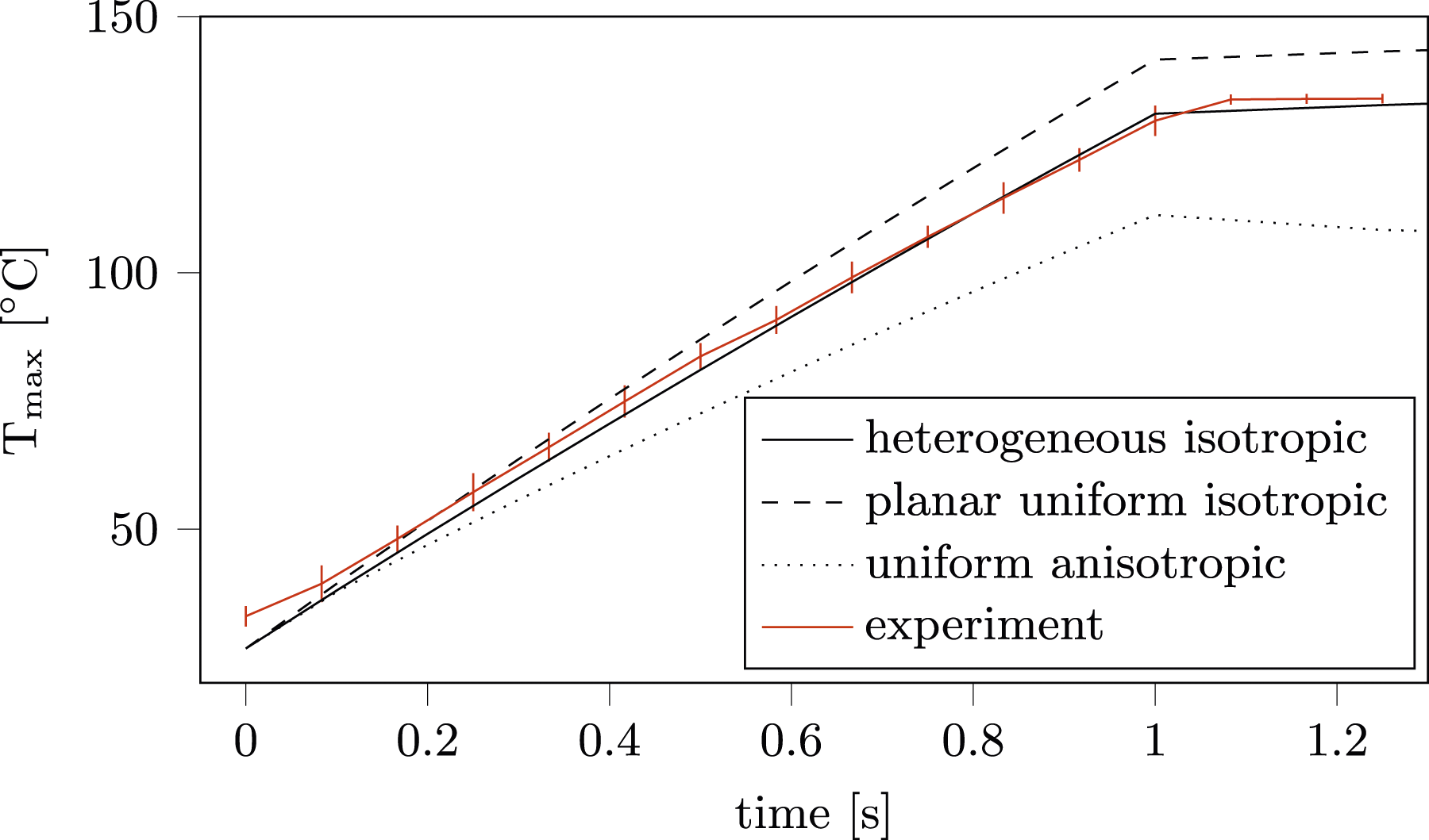

The maximum temperatures and the heating rates are shown in Figure 18. The planar uniform isotropic electrical conductivity model consistently led to an overestimation of maximum temperature and, consequently, the heating rate for all coil orientations. Furthermore, an insensitivity to the coil orientation can be seen in Figure 18. The uniform anisotropic electrical conductivity model showed a temperature prediction that was sensitive to the coil orientation, but the maximum temperature predictions and heating rates were underestimated for all coil orientations except for θ = 45°.

Figure 18.

Comparison of simulated and measured temperature data: (a) maximum temperatures at one second of heating; (b) heating rates between 0.1 and 0.9 s of heating.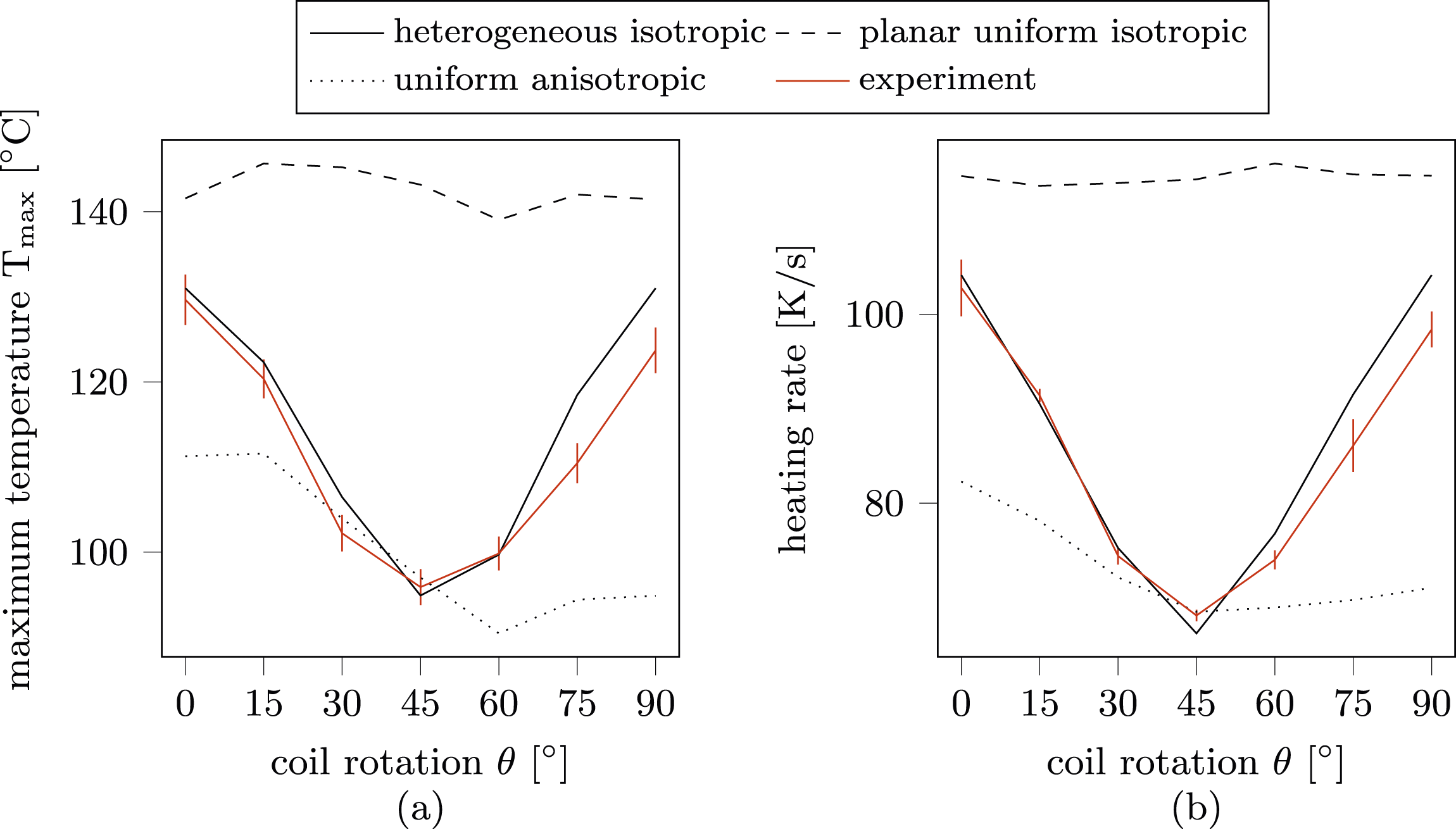

Discussion

Current density distribution predictions

Figure 7 shows that the current density distributions at the bottom surface of the laminate significantly differs between the different electrical conductivity models. The planar uniform isotropic electrical conductivity model is reflected in the predicted current density distributions, of which the magnitude is largely unaffected by the orientation of the induction coil.

The uniform anisotropic conductivity model provides a current density distribution that may be more complex to interpret. As a result of splitting the plies into two UD layers, the current density field is also split across these layers. The current density distributions displayed in Figure 7 are the predictions at the location of the bottom surface of the laminate in the models. As the UD-layer responsible for the electrical conductivity in the first principal direction is located at this surface in the model (see Figure 5), high current densities are predicted when currents are generated primarily in this direction (see current densities distributions predicted for θ < 45°). Similarly, when higher currents are generated in the second principal direction (for θ > 45°), the upper UD-layer of this bottom ply would display high current densities, while the lower layer shows low values as can be seen in Figure 7 for θ > 45°.

The current density distributions predicted by the heterogeneous isotropic method for defining the electrical conductivity were found to be symmetric about the 45° axis. This is evidenced by the mirrored current density values across θ = 0° and 90°, θ = 15° and 75° and θ = 30° and 60°.

Temperature predictions

The heterogeneous isotropic electrical conductivity (Figures 9–18) provides more accurate temperature predictions than the other two electrical conductivity models for the given experimental conditions. This is because the induced currents are mainly in-plane oriented, due to the low electrical conductivity in the laminate’s thickness direction and the applied magnetic load being predominantly perpendicularly oriented to the plane of the heated laminate. Therefore, an accurate in-plane electrical conductivity model is essential for accurate electromagnetic field predictions. The heterogeneous isotropic electrical conductivity model relies on a measured effective in-plane electrical conductivity, in contrast to the planar uniform isotropic and uniform anisotropic electrical conductivity models, which rely on calculated in-plane electrical conductivities (whether anisotropic or isotropic).

The inaccuracy in the temperature predictions is easily understood in the case of the planar uniform isotropic electrical conductivity model: this method results in an isotropic predicted thermal response to the imposed alternating magnetic field due to the isotropic in-plane electrical conductivity in this method. The reason that the temperatures are consistently overestimated is caused by the in-plane electrical conductivity being equal to the electrical conductivity in the direction of the fibre bundles in all directions. However, electrical conductivity measurements show that the effective in-plane electrical conductivity decreases as the direction deviates further from the direction of the fibre bundles. This can be approximated, for example, by equation (6), with a minimum at θ = 45° in the case of a balanced fabric as fibre reinforcement in the TPC material.

The temperature predictions using the uniform anisotropic electrical conductivity model revealed a dependence on the orientation of the coil, and thus the direction in which the electrical currents were predominantly induced within the laminate. This directional dependency, however, was less pronounced in comparison to the experimental results, this can be seen in Figure 18. Furthermore, the thermal response to the applied magnetic field was hardly symmetric around the 45° coil orientation, as best seen in Figure 18(b). The heating rate for θ > 45° was predicted to be lower compared to the heating rates for θ < 45°. The underlying reason is that for θ > 45°, the eddy currents were mainly induced in the σ₂ layers (see Figure 5). Consequently, the Joule heating mainly occurred in these layers. This heat was then dissipated to the σ₁ layers, resulting in a lower heating rate for those layers and thus in the monitored bottom surface of the heated laminate in the FE model since this surface was located in a ‘σ₁-layer’.

A more homogeneous thermal response in the ply’s thickness direction could possibly be obtained by increasing the number of UD-layers to represent the fabric ply. However, aside from the increased computation cost resulting from the increased number of UD-layers in the numerical model, this has another more stringent effect on the approximated anisotropic in-plane electrical conductivity. Adding more UD-layers implicitly increases the interface surface between the UD-layers in the fabric ply. As a result, the approximated in-plane electrical conductivity becomes less anisotropic, and therefore less accurate, with increasing number of UD-layers and at a constant value for σ₃, which in turn comes at the expense of the accuracy of the transient temperature predictions.

Another aspect of the uniform anisotropic electrical conductivity model is its strong dependence on the out-of-plane electrical conductivity, which is the crucial parameter to couple the electrical conductivities of the two UD-layers to obtain an accurate approximation of the effective anisotropic electrical conductivity of the fabric ply. However, the out-of-plane electrical conductivity is often difficult to measure accurately,^6,20 and it significantly depends on the fabric architecture and V_f. This leads to inaccuracy of the approximated in-plane anisotropy of the electrical conductivity, which in turn results in inaccurate temperature predictions.

In agreement with previous studies using the uniform anisotropic electrical conductivity to define the fabric ply’s anisotropic electrical conductivity, no electrical conductivity (σ₂ = 0) was applied in the UD-layer’s second principal direction. This value is rather arbitrary, as one could argue that σ₂ = σ₃ should be used instead. This assumption is probably reasonable for an actual UD ply, but in contrast to an actual UD ply, the crossing fibre bundles within the fabric provide for an increased electrical conductivity. This means that there is some electrical conductivity in the second principal direction, although it is likely to be much lower than the electrical conductivity in the first principal direction. In reality, a correct value for σ₂ in the uniform anisotropic electrical conductivity model cannot be directly validated or characterized by experiments.

Conclusions

The overall objective of the present study is to determine whether a heterogeneous isotropic description of a measured anisotropic in-plane electrical conductivity of a balanced woven fabric reinforced TPC can be used to correctly predict the thermal response of a TPC laminate when heated by induction.

It was shown that the transient temperature distribution predictions show good agreement with temperature measurements from corresponding induction heating experiments using the heterogeneous isotropic electrical conductivity model in numerical induction heating simulations. Using the heterogeneous isotropic electrical conductivity model, the induction heating simulations in this study:

• demonstrate a good qualitative agreement between the predicted temperature field and the measured temperature field. The results indicate that the induction heating simulations using the heterogeneous isotropic electrical conductivity model is able to capture the temperature field with higher accuracy compared to the planar uniform isotropic and the uniform anisotropic electrical conductivity models;

• provide evidence of strong agreement between predicted and observed heating rates for the directions in which electrical currents were predominantly generated by induction;

• show a high degree of agreement between the maximum temperature predictions and the measured maximum temperatures.

Footnotes

Acknowledgements

The authors gratefully acknowledge the support from the industrial and academic members of the ThermoPlastic composites Research Center (TPRC).

Declaration of conflicting interests

The author(s) declared no potential conflicts of interest with respect to the research, authorship, and/or publication of this article.

Funding

The author(s) disclosed receipt of the following financial support for the research, authorship, and/or publication of this article: This work was supported by the industrial and academic members of the TPRC.

ORCID iDs

Sebastiaan van den Berg

Martin Luckabauer

Remko Akkerman

References

Appendix

Figure 19.

Applied in-plane electrical conductivities for coil orientations θ = 60°, 75° and 90°.

References

Airbus . Global market forecast; cities, Airports and Aircraft; 2019-2028. Technical report. AIRBUS S.A.S., 2019.

Ingen van

Buitenhuis

Wijngaarden van

, et al. Development of the Gulfstream G650 induction welded thermoplastic elevators and rudder, 2010.

Holland

van Tooren

Barazanchy

, et al. Modeling of induction heating of thermoplastic composites. J Thermoplast Compos Mater 2022; 35(10): 1772–1789.

Mitschang

Rudolf

Neitzel

. Continuous induction welding process, modelling and realisation. J Thermoplast Compos Mater 2002; 15(March): 127–153.

Hoffman

Becker

Duhovic

, et al. Simulating the induction heating behavior of CFRTPC laminates. In: 13th European LS-DYNA Conference, Kaiserslautern, October 5-7, 2021, 202116, DYNAmore GmbH, vol.

Lundström

Frogner

Andersson

. Analysis of the temperature distribution in weave-based CFRP during induction heating using a simplified numerical model with a cross-ply representation. Compos B Eng 2021; 223: 109153.

Berg van den

Luckabauer

Wijskamp

, et al. Thermal response of an induction-heated fabric reinforced thermoplastic composite with anisotropic electrical conductivity: an experimental study. J Thermoplast Compos Mater 2024; 37(5): 1877–1892.

Fink

Mccullough

Gillespie

. A model to predict the planar electrical potential distribution in cross-ply carbon-fiber composites subjected to alternating magnetic fields. Compos Sci Technol 1993; 49: 71–80.

Kim

Yarlagadda

Shevchenko

, et al. Development of a numerical model to predict in-plane heat generation patterns during induction processing of carbon fiber-reinforced prepreg stacks. J Compos Mater 2003; 37(16): 1461–1483.

10.

Grouve

WJB

Sacchetti

Vruggink

, et al. Simulating the induction heating of cross-ply C/PEKK laminates–sensitivity and effect of material variability. Adv Compos Mater 2020; 30: 409–430.

11.

Wit de

Hoorn van

Nahuis

, et al. Prediction of thermo-mechanic effects through numerical simulation of induction heating of thermoplastic composites. Technical Report NLR-TP-2021-491. Amsterdam: Royal NLR, 2022.

12.

Bensaid

Trichet

Fouladgar

. 3-D simulation of induction heating of anisotropic composite materials. IEEE Trans Magn 2005; 41(5): 1568–1571.

13.

Moser

. Experimental analysis and modeling of susceptorless induction welding of high performance thermoplastic polymer composites. Thesis. Technische Universität Kaiserslautern, 2012.

14.

Pappadà

Salomi

Montanaro

, et al. Induction welding of pps-carbon composites: modeling and experimental results. In ICCM International Conferences on Composite Materials, Montréal, Canada, 2013, 2013-July, 5481–5488.

15.

Duhovic

Moser

Mitschang

, et al. Simulating the joining of composite materials by electromagnetic induction. Simulating the Joining of Composite Materials by Electromagnetic Induction 2014; 2: 1–22.

16.

Kim

Yarlagadda

Gillespie

, et al. A study on the induction heating of carbon fiber reinforced thermoplastic composites. Adv Compos Mater 2002; 11(1): 71–80.

17.

Toray Advanced Composites . Toray cetex TC1320 PEKK. Technical Report 3. Nijverdal, Netherlands: Toray Advanced Composites, 2019.

18.

COMSOL Multiphysics® . v. 6.1. Stockholm, Sweden: COMSOL AB, www.comsol.com

19.

Becker

Michel

Mitschang

, et al. Influence of polymer matrix on the induction heating behavior of CFRPC laminates. Compos B Eng 2022; 231(December 2021): 109561.

20.

Berg van den

Luckabauer

Wijskamp

, et al. Determination of the anisotropic electrical conductivity of carbon fabric reinforced composites by the six-probe method. J Thermoplast Compos Mater 2023; 36(11): 4257–4283.

Simulating induction heating of fabric based thermoplastic composites using measured electrical conductivities

Abstract

Keywords

Introduction

Experimental work

Model set-up

Equations

Implementation of the electrical conductivity

Material properties

Geometry and discretisation

Loads and boundary conditions

Validation models

Simulation results

Computation times

Apparent in-plane electrical conductivity fields

Temperature distribution

Discussion

Current density distribution predictions

Temperature predictions

Conclusions

Footnotes

Acknowledgements

Declaration of conflicting interests

Funding

ORCID iDs

References

Appendix

References