Sage Journals: Discover world-class research

Abstract

A computationally efficient heat transfer simulation of flashlamp-assisted automated tape placement (ATP) is put forward in this work. The simulation combines distinct 1D finite element models representing the tow, the deposited material, and the resulting stack with appropriate transfer of temperature information to ensure field continuity. Direct comparison against a validated 2D model of ATP shows good agreement in the irradiation region, underneath and beyond the roller vicinity with errors up to 14°C. The combined solution of 1D models requires only 1-2% of the computational effort needed for an equivalent 2D analysis without compromising results resolution, whilst it is better suited for providing the full material temperature history throughout consecutive processing cycles. The accuracy and fast computation render this method appealing for studies which require an iterative execution of the model in a practical timeframe such as in optimisation schemes, inverse solutions, training of surrogate models and stochastic simulation.

Keywords

finite element analysis process modelling thermoplastics tape placement pulsed heating

Introduction

Automated tape placement (ATP) is an additive manufacturing method in which robotic equipment is utilised to deposit layers of continuous fibre-reinforced composite tapes onto a tool. A radiative energy source raises the temperatures of the already deposited material and the new layer moments before they come into contact underneath a compaction roller, facilitating part consolidation and bonding between layers. The consistency of automated processes and potential of building large composite parts at high rates render this method very attractive for aerospace applications. This vision is led to a great extent by the utilisation of thermoplastic-based composites, which can be processed in a single step mitigating the long and time-consuming autoclave cycles involved in thermosetting matrix composite processing. However, further research is required before the strict quality and production criteria are met.

The importance of the temperatures developed inside the process on the final part quality has been highlighted in numerous studies,^1–7 and as a result the heat transfer analysis of ATP has received significant attention.⁸ Up to three-dimensional methodologies have been developed,^9–12 with most works reducing the problem to two dimensions assuming uniform heating across the tape width.^13–25 The heat conduction in the direction of placement has been neglected compared to the heat transport due to rapid material movement, as indicated by the high Peclet number for the tapes and high velocities typically used.^15,21,26 The latent heat due to matrix transformations has been included in the analysis in some cases;^15–20 however, the contribution of these exothermic/endothermic effects has been considered negligible when compared to the high energy input by the heater.^21–25 One-dimensional numerical and analytical models have been introduced, simplifying the process to a through-thickness material slab.^26–29 Surrogate and neural network models have also been presented, trained by a high number of numerical solutions.^30,31 Most models have adopted a Eulerian coordinate system mounted on the moving placement head,^{15,16,18–25} whereas others have been based on a Lagrangian system.^14,17

Computation time is critical for schemes which require a high number of iterative runs. 1D methodologies typically require much lower computational effort, but also involve major assumptions which hinder accuracy.^26–29 An approach based of decomposing the 2D domain to 1D subdomains has been put forward; however, the effects of contact between the composite and the roller and its dynamic character have not been taken into account.²⁶ The heat exchange between the tow and deposited material has been simplified by averaging their temperatures at the nip point.²⁸ Simplifications on other aspects regarding the roller, temperature-dependent material properties and non-homogeneous irradiance distribution on the tapes have also been applied. Fast surrogate and neural network models have been proposed; however, a large number of simulations is required for training to establish these representations.^30,31 Although existing 2D methodologies use fewer assumptions compared to 1D models, obtaining the material temperature history across the whole geometry, and for all depositions, presents a significant computational challenge. A small portion of the overall part is usually modelled, due to the computational effort required to represent large geometries with fine discretisation.^22,25 The smaller domain of the Eulerian approach, adopted by the majority of studies, provides efficient solutions in the vicinity of the nip point at a loss of the temperature evolution outside this analysis frame. The analysis follows the deposition head, solving the boundary problem for a narrow time window spanning typically from the irradiation zone start to some extent outside the roller contact patch. Predicting the temperature evolution for a period of 5–10 s at 100 mm/s requires an analysis domain which is 500–1000 mm long. Such timings are well within the timeframe of critical material phenomena taking place such as degradation, crystallisation, and bonding development, as well as curing for thermosetting materials. Solving for a large enough geometry to capture these effects impacts computational times severely. In addition, without the full material temperature history, residual heating effects in the stack cannot be included, which is critical for manufacturing programs in which cooling to ambient conditions before a new deposition is not achieved.

Up to date, efforts focus on ATP processes deploying continuous heating sources such as lasers, IR heaters and hot gas torches. Recently, pulsed sources based on Xenon-filled flashlamps have become available for ATP. The heat transfer of flashlamp-assisted ATP, combined with ray tracing analysis, has been addressed.²⁵ The short high-energy pulses of the heater, in the range of 0.5–5 ms, impose a much finer time discretisation than typically used for simulating continuous sources. Solution times in the range of 1-2 hrs are required for a typical 2D Eulerian analysis frame about 100 mm in length,²⁵ indicating the need for improvements in computational efficiency before the model can be used for iterative execution and extended processing cycles.

In this study, an 1D simulation of flashlamp-assisted ATP is put forward which uses a combination of 1D submodels to address the tow and deposited material heating, and their interaction under and beyond the compaction roller. The transfer of temperature information among the models ensures thermal field continuity. The methodology is applicable to pulsed sources offering a universal heat transfer solution for integration in process modelling schemes. The accuracy of the method is assessed against a validated 2D model of flashlamp-assisted ATP²⁵ for a wide range of processing rates, deposited material thicknesses and heater pulsing conditions. The improvements in computational efficiency are examined for a wide variety of processing scenarios. The results of the 1D model are set against monitoring data obtained during AFP trials to validate the approach with respect to the physical process.

Model formulation

The full ATP problem can be considered two-dimensional by assuming uniform heating across the tape width and no edge effects. The latent heat due to matrix transformations can be considered negligible due to the low crystallinity levels typically achieved in ATP and the polymer constituting only 30–35% of tape mass. For a Eulerian frame attached on the moving placement head and material motion aligned with the local x-coordinate, the energy balance is:

ρ c_{p} (\frac{\partial T}{\partial t} + u_{x} \frac{\partial T}{\partial x}) = \frac{\partial}{\partial x} (k_{x} \frac{\partial T}{\partial x}) + \frac{\partial}{\partial y} (k_{y} \frac{\partial T}{\partial y})

(1)

where

T

denotes temperature,

ρ

the density of the composite,

c_{p}

the specific heat capacity,

k_{x}

and

k_{y}

the thermal conductivity in the placement and thickness direction respectively and

u_{x}

the placement velocity.

Heat conduction in the composite in the placement direction has been found to be negligible compared to the heat transport by material motion, as a result of the rapid material movement and relatively low longitudinal thermal conductivity of typical thermoplastic-based composite tapes, manifested as high values of the Peclet number. Values of the Peclet number lower than unity can occur during the first moments of the process under very slow velocities, but this condition holds true for a short period of time compared to the duration of the placement process. As a result, the heat transport due to material advection dominates in the placement direction and equation (1) becomes:

ρ c_{p} (\frac{\partial T}{\partial t} + u_{x} \frac{\partial T}{\partial x}) = \frac{\partial}{\partial y} (k_{y} \frac{\partial T}{\partial y})

(2)

This 2D transient energy balance can be transformed to an 1D transient state equation by applying the transformation

x^{'} = x - u_{x} t

to obtain:

ρ c_{p} (\frac{\partial T}{\partial t}) = \frac{\partial}{\partial y} (k_{y} \frac{\partial T}{\partial y})

(3)

This transforms the analysis reference frame from Eulerian to Lagrangian, in which the solution corresponds to a fixed material point, with the surface of the material subjected to a time-dependent heat flux input. Equation (3) is a valid representation of heat transfer in ATP due to the negligible heat diffusion in the placement direction, which renders the through-thickness conduction the dominant heat transfer mechanism.

Applying the principle expressed by equation (3) to the 2D representation of ATP in Figure 1, three different submodels can be identified each addressing a different process region. Model I and Model II describe the temperature evolution in a material slice belonging to the deposited material and the incoming tow respectively, as they are irradiated prior to the nip point. Model III represents the heat transfer from the moment the deposited material and incoming tow slices come into contact underneath the compaction roller, until the end of the stage where the stack has been left to cool down at ambient conditions.

Figure 1.

2D representation of heat transfer in ATP and identification of 1D submodels for the deposited material (Model I), incoming tow (Model II) and consolidation zone (Model III).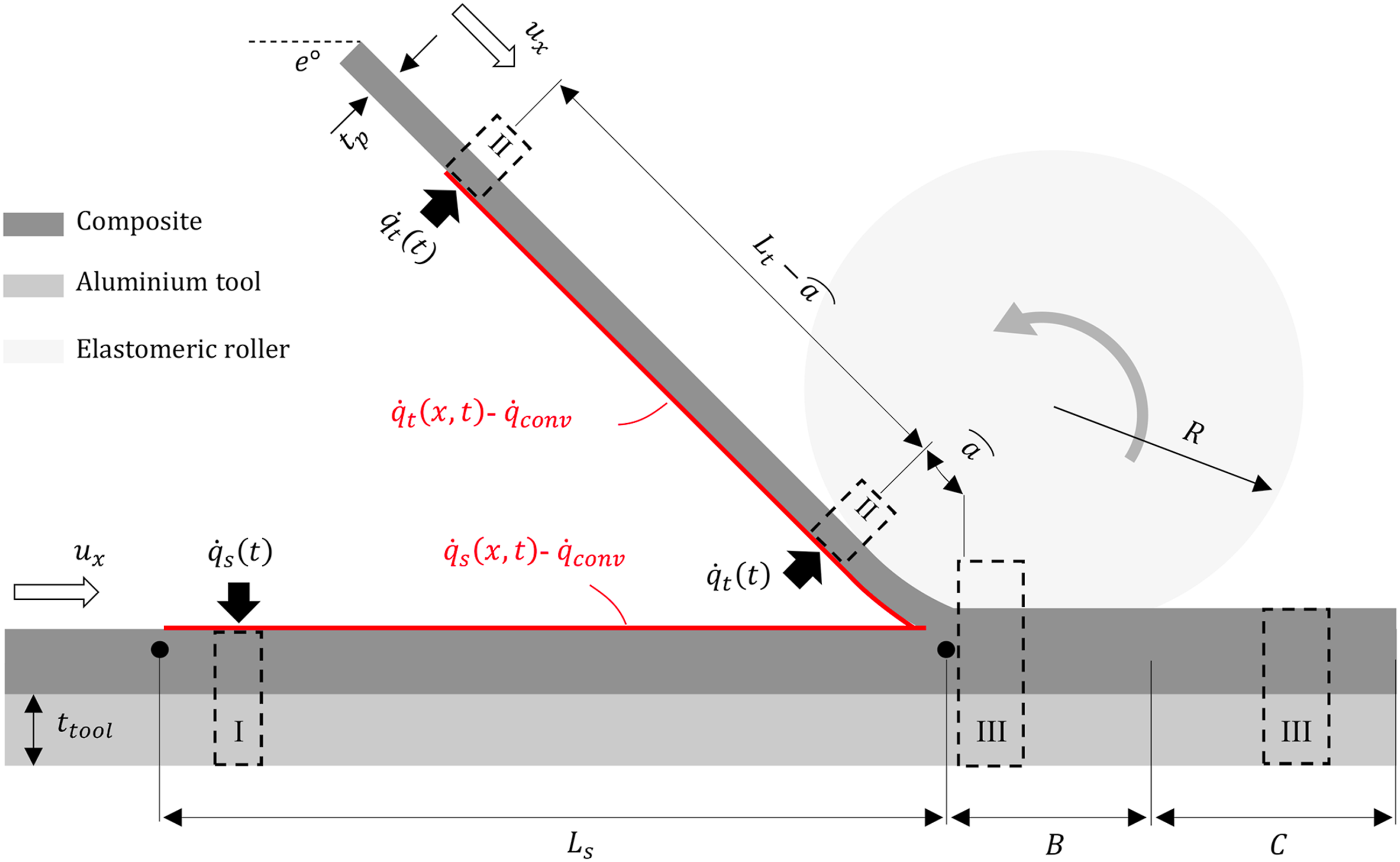

Model I–deposited material

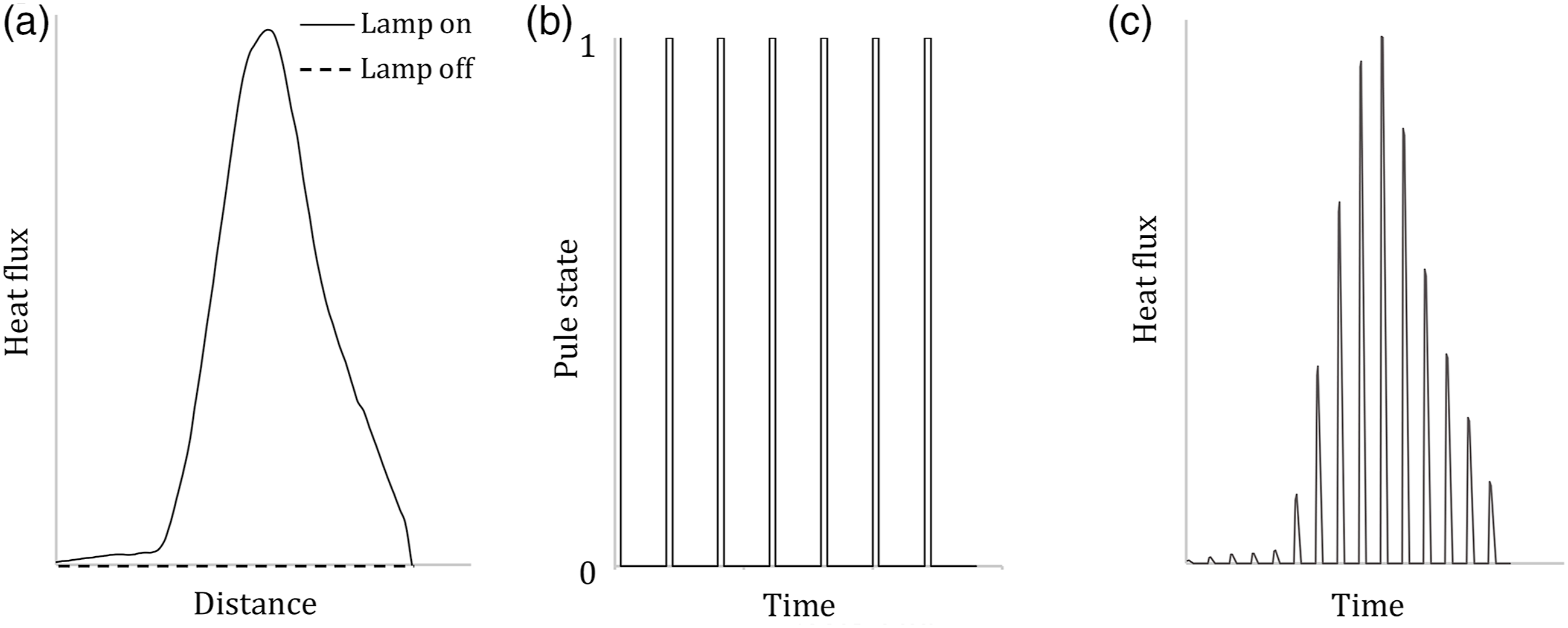
Model I represents the deposited composite material consisting of $n$ composite tape layers in perfect contact with the process tool. The submodel analysis time is equal to the distance covered from the irradiation start to the nip point, $L_{s}$ as indicated in Figure 1, divided by the placement velocity. An overview of the applied boundary conditions is provided in Figure 2(a). The surface of the composite material is irradiated by the heating source and as a result it is subjected to a combined boundary condition of heat flux and convection to air:

k_{y} \frac{\partial T}{\partial t} = q_{s} (t) - h (T_{s u r} - T_{a m b})

(4)

where

T_{a m b}

is the ambient temperature,

h

the surface heat transfer coefficient and

T_{s u r}

the surface temperature. Term

q_{s} (t)

represents the transformed spatial irradiance distribution on the deposited material surface prior to the nip point (Figure 1) resulting from the transformation from a Eulerian to a Lagrangian system (

x^{'} = x - u_{x} t)

. For pulsed sources, the non-continuous operation is accounted in

q_{s} (t)

by convoluting the profile with a train of rectangular pulses of desired frequency and duration. The resulting heat flux is effectively the irradiation history of a single point moving across the irradiation zone under a non-continuous source. A schematic of this procedure is provided in Figure 3. In addition, convection to ambient conditions is applied to the back surface of the tool:

k_{y} \frac{\partial T}{\partial t} = h (T_{s u r} - T_{a m b})

(5)

Figure 2.

Materials and boundary conditions of 1D submodels: (a) Model I (deposited material); (b) Model II (tow) no thermal contact with roller, (c) Model II in contact with roller; (d) Model III (consolidation zone) underneath roller; (e) Model III outside the contact region.

Figure 3.

Determination of 1D simulation heat flux input: (a) spatial irradiance acting on tape surface; (b) pulse train of desired frequency and pulse duration; (c) corresponding heat flux for use in Model I and Model II for a given velocity.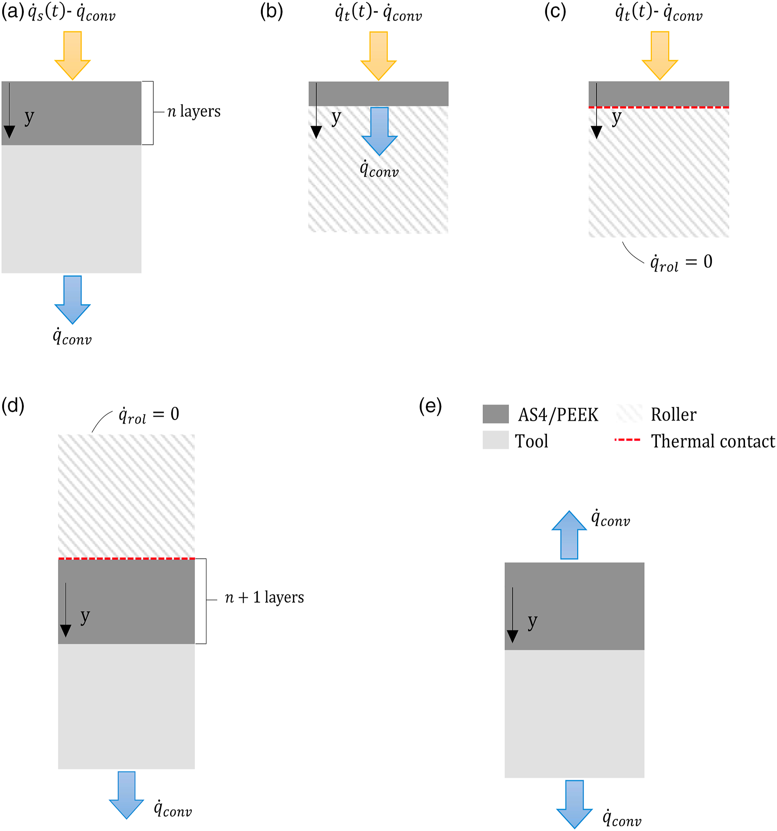

Model II–incoming tow

Model II represents a single composite layer into contact with a compaction roller which features a reduced geometry (Figure 2(b) and (c)). The submodel analysis time is equal to the distance covered from the irradiation zone entry to the nip point, $L_{t}$ as indicated in Figure 1, divided by the placement velocity. The irradiation path consists of a straight line and a curved part which follows the roller geometry (Figure 1) and has an arc length $\hat{a}$ . In the transient analysis expressed by equation (3), heat conduction between the tape and the roller is not active throughout the whole analysis. Heat transfer between the two bodies is activated at a time which corresponds to the arrival time of a point moving from the irradiation start to the roller contact point, equal to $t = (L_{t} - \hat{a}) / u_{x}$ (Figure 1). A thermal contact of negligible resistance between the nodes belonging to the tow-roller interface is created at this time.

Two sets of boundary conditions are applied in Model II (Figure 2(b) and (c)) as a result of the tow-roller contact established during the analysis. A combined boundary condition of heat flux and convection acts on the surface of the tow during both analysis stages:

k_{y} \frac{\partial T}{\partial t} = q_{t} (t) - h (T_{s u r} - T_{a m b})

(6)

where

q_{t} (t)

in this case represents the converted spatial irradiance distribution on the tow surface similarly to

q_{s} (t)

in equation (5). During the analysis stage where the contact with the roller is not active (Figure 2(b)), the tow back surface is subjected to air convection with a constant coefficient (equation (5)). Once the tow-roller thermal contact has been established, convection is no longer applied (Figure 2(c)). The roller is treated as a semi-infinite body following from its Fourier number which is lower than one for a slice thickness of 5 mm, elastomer conductivity of 0.2 W/m/K and representative contact time with the tow of 1 s. Shorter times lead to lower Fourier numbers strengthening the validity of this assumption. As a result, the interior boundary of the semi-infinite roller is treated as insulated:

\frac{\partial T}{\partial y} = 0

(7)

Model III–consolidation zone

Model III represents the resulting composite stack after the incoming tow and the deposited material come into contact at the nip point underneath the compaction roller (Figure 2(d) and (e)). The composite consists of $(n + 1)$ layers. The roller and tool have identical geometries as in Models I and II, whilst the interlayer resistance between plies is considered negligible. Unlike Model II, a thermal contact between the nodes at the composite-roller interface is active from the beginning of the analysis and it is deactivated at later steps, according to the contact patch length $B$ and processing velocity (Figure 1).

Two sets of boundary conditions are applied in Model III due to the loss of contact between the composite and the roller during the analysis. Only natural convection is applied to the tool back surface during the contact stage (Figure 2(d)). Similarly to Model II, the roller is treated as a semi-infinite body and thus an adiabatic boundary exists on its inner surface (equation (7)). After loss of contact, the stack is left to cool down at ambient conditions and thus natural air convection is applied on its surface.

Integration of the three 1D models

The analysis sequence and information flow between the 1D submodels is outlined in Figure 4. Once the solution of Models I and II has been completed, the resulting through-thickness temperature distributions are transferred as initial temperature conditions in Model III (Figure 4(a)), ensuring field continuity between the irradiation and consolidation zones. The temperature of the tow-deposited material interface at the nip point ( $x = 0$ ) is set as the average value of the surface nodes in Models I and II. At the end of the processing cycle, the temperatures across the thickness of Model III can be transferred to a new Model I (Figure 4(b)) which represents an additional layer. In this way, multiple placements are simulated taking into account the residual heating when complete cooling of the stack to ambient conditions has not been completed. Model II is solved once and used in the prediction of multiple placement cycles since the tow irradiation is independent of the increasing deposited material thickness. A heated tool or preheated tow can be simulated by fixing or initialising the temperature of the nodes belonging to the tool and tow, respectively, to a constant value in the corresponding 1D models.

Figure 4.

Operation of the integrated 1D simulation: (a) solution sequence and temperature data exchange among the different submodels; (b) workflow for modelling multiple placement cycles including residual heating. Ti (y,t) denotes temperature at position y across the thickness of submodel i at time t.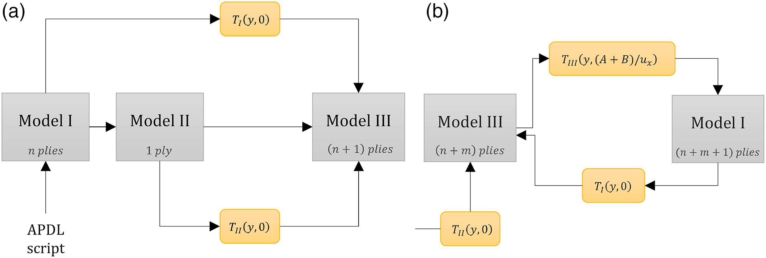

Methodology

A comparison between the predictions of the 1D simulation put forward in this study and a 2D finite element model previously validated against temperature measurements in ATP process trials²⁵ is carried out here. The computational effort needed by each model to provide solutions is also compared, as benchmarked by the finite element solver for each run. Both models were implemented in Ansys APDL using the distributed memory parallel processing option within a single 4-core PC (i7-4790). This solving mode decomposes the model into smaller domains, solves them simultaneously by assigning each to a single core, and then reconstructs the complete solution. This mode accelerates the solution compared to Shared-memory parallel processing (SMP), especially for the 2D model due to an overall larger domain. The default sparse direct solver was chosen which balances performance and accuracy.

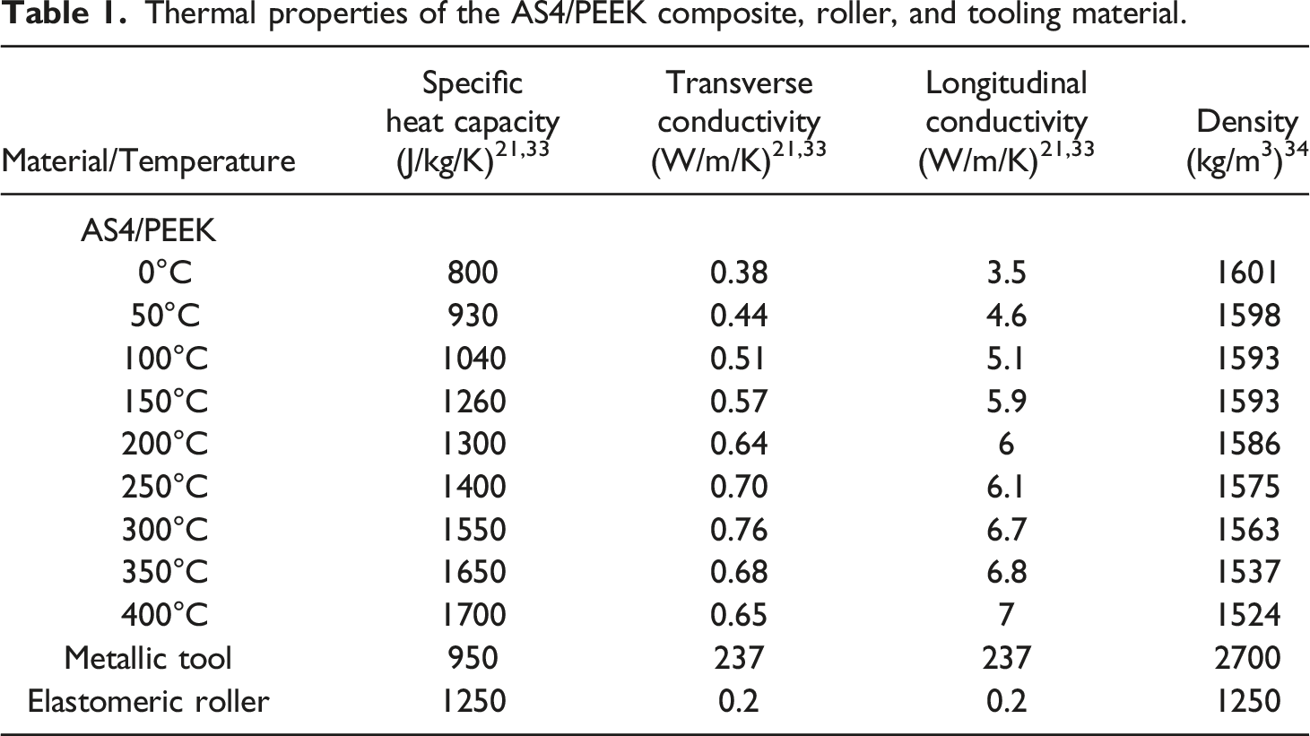
A Heraeus Noblelight humm3 system³² of 4.4 kW maximum power was used as the heater for this assessment. The flashlamp source features a pulsed operation with energy pulses in the 0.5–6 ms range and repetition rates up to 150 Hz. Two significantly different pulsing conditions of 25 Hz frequency 4.75 ms pulse duration and 100 Hz frequency and 1.1 ms pulse duration were investigated, both utilising the full system power capacity.²⁵ The composite material used for the placement process was a 0.18 mm thin unidirectional AS4/PEEK tape. The tool and roller thicknesses were set at 10 and 5 mm respectively. The thermal properties of AS4/PEEK tape,^21,33,34 the metallic tool, and the elastomeric roller are detailed in Table 1.

Table 1.

Thermal properties of the AS4/PEEK composite, roller, and tooling material.

Material/Temperature	Specific heat capacity (J/kg/K)^21,33	Transverse conductivity (W/m/K)^21,33	Longitudinal conductivity (W/m/K)^21,33	Density (kg/m³)³⁴
AS4/PEEK
0°C	800	0.38	3.5	1601
50°C	930	0.44	4.6	1598
100°C	1040	0.51	5.1	1593
150°C	1260	0.57	5.9	1593
200°C	1300	0.64	6	1586
250°C	1400	0.70	6.1	1575
300°C	1550	0.76	6.7	1563
350°C	1650	0.68	6.8	1537
400°C	1700	0.65	7	1524
Metallic tool	950	237	237	2700
Elastomeric roller	1250	0.2	0.2	1250

An overview of the assumptions of the two methodologies (1D and 2D) is presented in Table 2. The 2D model features the geometry of Figure 1 with key dimensions detailed in Table 3. It follows equation (1) and as a result the heat diffusion in the placement direction is taken into account. In contrast, the 1D simulation assumes this effect is negligible (equation (2)). Material advection in a Eulerian analysis frame is included in the 2D analysis by activating the mass transport effects for the PLANE292 element in APDL.³⁵ Two-node LINK33 elements were used in the 1D simulation. The convection coefficient is set at 5 W/K/m² in both models.

Table 2.

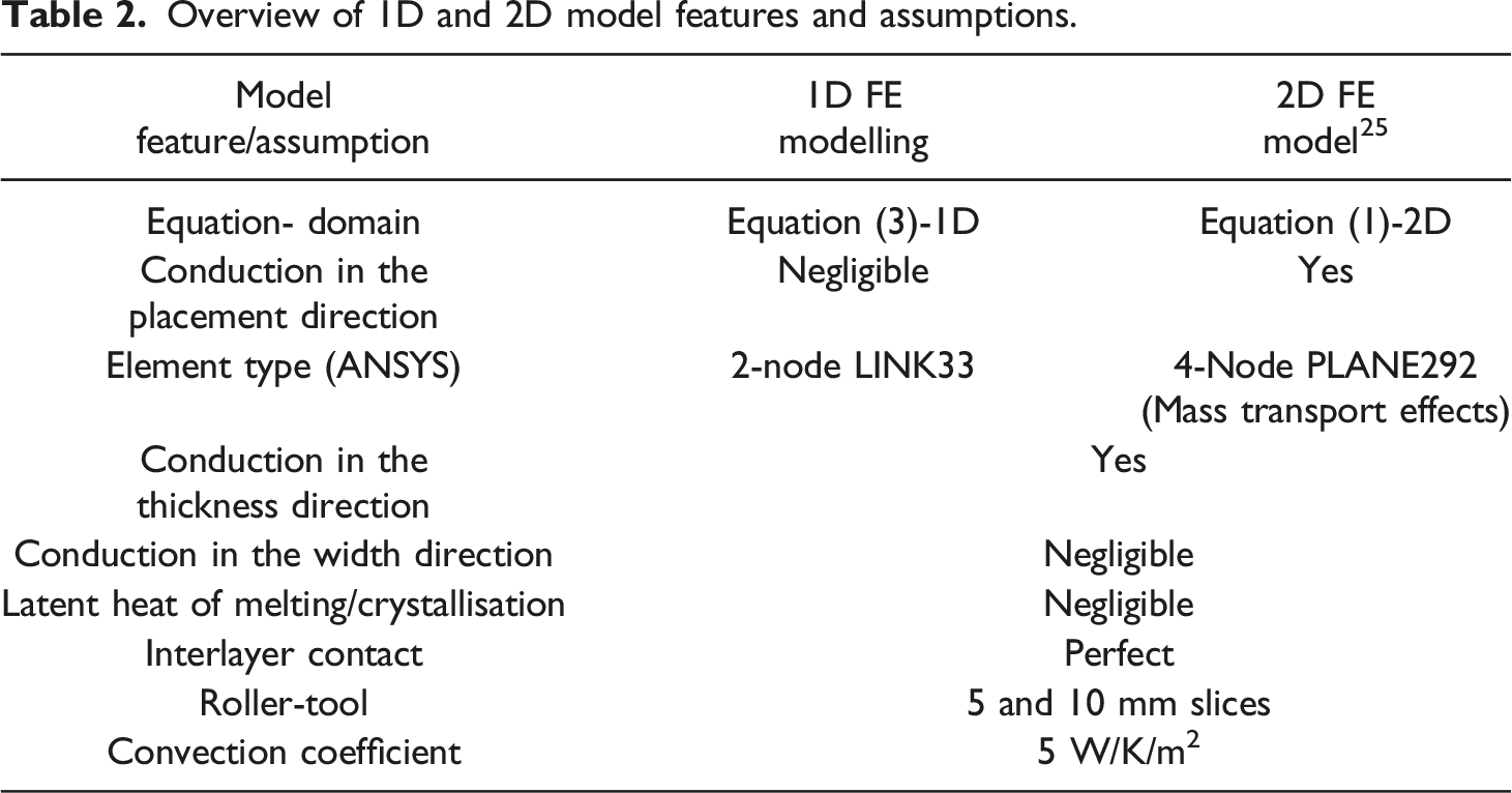
Overview of 1D and 2D model features and assumptions.

Model feature/assumption	1D FE modelling	2D FE model²⁵
Equation- domain	Equation (3)-1D	Equation (1)-2D
Conduction in the placement direction	Negligible	Yes
Element type (ANSYS)	2-node LINK33	4-Node PLANE292 (Mass transport effects)
Conduction in the thickness direction	Yes
Conduction in the width direction	Negligible
Latent heat of melting/crystallisation	Negligible
Interlayer contact	Perfect
Roller-tool	5 and 10 mm slices
Convection coefficient	5 W/K/m²

Table 3.

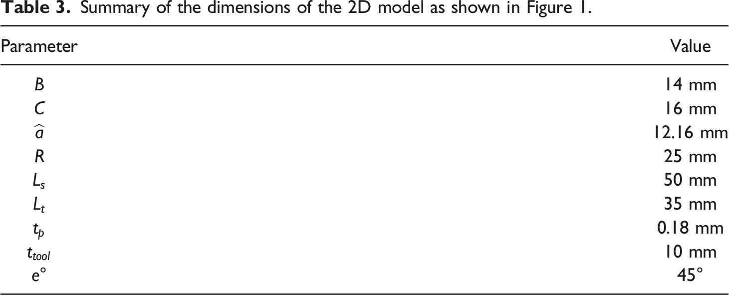
Summary of the dimensions of the 2D model as shown in Figure 1.

Parameter	Value
$B$	14 mm
$C$	16 mm
$\hat{a}$	12.16 mm
$R$	25 mm
$L_{s}$	50 mm
$L_{t}$	35 mm
$t_{p}$	0.18 mm
$t_{t o o l}$	10 mm
e°	45°

The two simulations share similar mesh grids in the through-thickness direction. The high heat flux applied during an energy pulse necessitates a fine through-thickness element size of 10 μm. However, refining a thin material slice close to the surface is sufficient to reach convergence.²⁵ The thickness of this slice should be greater than the thermal penetration depth of the pulse given by: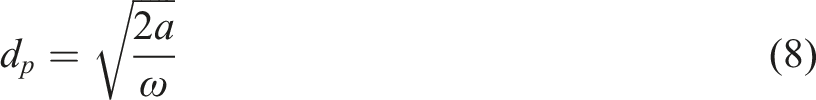

d_{p} = \sqrt{\frac{2 a}{ω}}

(8)

where

ω

is the angular frequency of the pulse and

a

the thermal diffusivity of the material in the thickness direction. A thickness of 150 μm was used for the fine mesh zone in all submodels. Outside this area, the periodic temperature variations become negligible and the temperature reaches a steady state that can be captured accurately by a coarser mesh in the 10–100 μm range. In the 2D implementation, the solver requires a very fine mesh in order to keep the Peclet number below one and solve equation (1), effectively rendering the heat diffusion in the placement direction essential for the solution at a given speed. The material of the lowest longitudinal conductivity, the roller in this case, governs the mesh size. Following the methodology established in a previous study,²⁵ the conductivity of the roller (Table 3) has been artificially increased 10 times to allow the use of 10 μm elements in the placement direction and keep solution times viable at higher velocities.

The total analysis time corresponds to the analysis frame length of 90 mm (Figure 1) divided by the processing speed. Each 1D submodel features a duration calculated based on the length of the corresponding stage it describes and the velocity. The simulation time has been discretised into steps with sufficiently short duration to model individual pulses. Two steps per period have been used to describe the pulsed operation: one for the pulse event and one for the remaining period time.²⁵ Although this results in fast computation for a given scenario, it can lead to inaccuracies due to insufficient number of points describing the non-linear heating/cooling curves in the pulse timescale, potentially influencing the outputs of material constitute models. Therefore, the choice should balance resolution and computation time. Here two load steps during the pulse and three during the cooling phase were used in both methodologies. The time increments within each load step are adjusted by the software to achieve convergence, until the square root of the sum of the squares (SRSS) of the residual vector is lower than the SSRR of the 0.1% of the applied fluxes or lower than 10⁻⁹. Model III does not involve pulsed heating and therefore longer timesteps of 10 ms were used.

The incident energy distribution acting on the tapes for the examined process configuration of Figure 1 has been estimated by a 3D ray tracing model for the specific flashlamp system.²⁵ The optical analysis included the ATP cavity and relevant system components such as the flashlamp tube, the water-filled cooling chamber, the quartz light guide, and the reflective housing. The predicted 3D irradiance distributions were reduced to a single profile across the tape middle line, after their post-processing with a Savitzky-Golay filter to smooth the data and eliminate outliers caused by the statistical nature of the ray tracing solution. The predicted spatial irradiance profiles acting on the tow and the deposited material surfaces are provided in Figure 5(a). The pulsed operation in the 2D model is simulated by activating the heat flux applied on the tape surface (Figure 1) according to the system frequency and pulse duration.²⁵ As a result, the acting heat flux oscillates between the maximum value and zero (Figure 5(a)). The corresponding heat flux profiles used in Model I and Model II are presented in Figure 5(b) and (c) respectively for a velocity of 50 mm/s. Processing rates affect the x-coordinate based on the Eulerian to Lagrangian transformation, and as a result the number of energy pulses delivered prior to the nip point.

Figure 5.

Heat flux input: (a) spatial distributions used in the 2D model; (b) profile applied on the composite surface in Model I; (c) profile applied on the tow surface in Model II. Placement at 50 mm/s under two different pulsing conditions. Nip point reached at t = 0 s.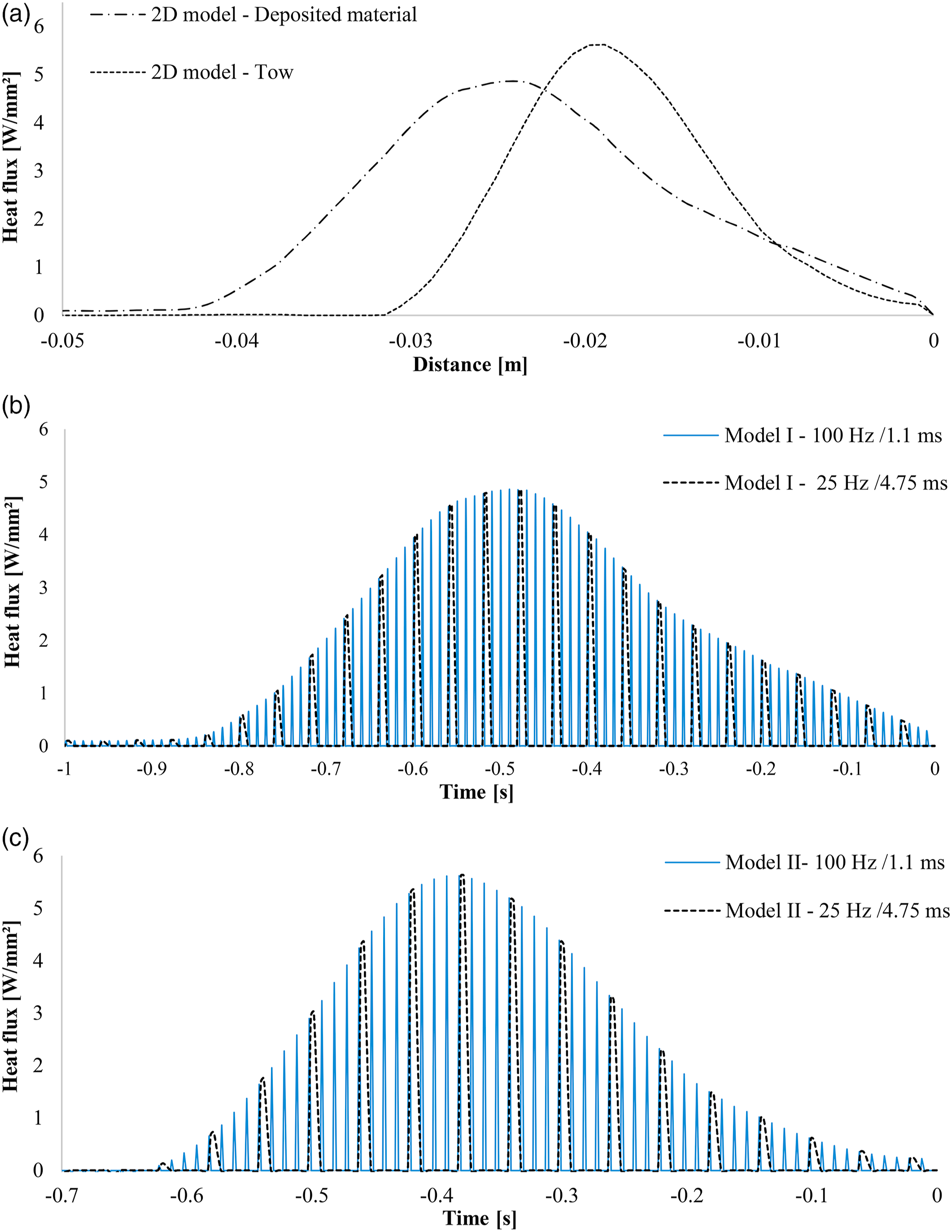

Results and discussion

Model I verification

A comparison of predicted temperatures by the 2D and 1D models for the deposited material surface (Model I) are illustrated in Figures 6 and 7. These are the highest temperatures expected in the deposited material, due to the applied surface heat flux, and therefore important for thermal degradation studies. The nip point is reached at $t$ = 0 s. The irradiation of the deposited material is examined during the 2^nd and 5^th layer placement under 25 Hz/4.75 ms (Figure 6) and 100 Hz/1.1 ms (Figure 7) pulsing conditions. The deposited material consists of one and four AS4/PEEK layers respectively. The predictions correspond to a velocity of 50 mm/s following the heat flux profiles of Figure 5(b). The surface temperatures comprise consecutive heating/cooling cycles with timings dictated by the input heat flux (Figure 5(b)). A closer look at a pulse timescale is illustrated in Figure 8. The heating phase is as long as the pulse whilst the repetition rate of the heating/cooling cycles is equal to the pulsing frequency. As a result, the material is subjected to more cycles at the higher frequency of 100 Hz. The longer pulses of the 25 Hz operation result in higher local maximum temperatures; however, these decrease to lower values at the end of the period due to the longer cooling times before a new energy pulse is delivered, 35.25 versus 8.9 ms. As the deposited material thickness increases, greater temperatures are developed on the surface since the deposited layers, which have a low transverse conductivity, act as an insulating barrier to the heat diffusion towards the metallic tool.

Figure 6.

Comparison of predictions on the surface of the deposited material at 50 mm/s: (a) 2nd layer placement and (b) 5th layer placement under 25 Hz/4.75 ms operation. Nip point reached at t = 0 s.

Figure 7.

Comparison of predictions on the surface of the deposited material at 50 mm/s: (a) 2nd layer placement and (b) 5th layer placement under 100 Hz/1.1 ms operation. Nip point reached at t = 0 s.

Figure 8.

Heating/cooling cycles during pulsing on the surface of the deposited material under two different source operations. Placement of 5th layer at 50 mm/s.

Model I predictions of surface temperatures on the deposited material are in close agreement with the results of the 2D model (Figures 6 and 7), with errors of up to 10°C. An average error of 2°C is present across all examined scenarios. The timings of the heating/cooling cycles created on the material surface are in full agreement (Figures 6–8) due to the exact time discretisation in steps. The greatest deviations occur at 25 Hz and for the 5^th ply placement due to the higher temperatures developed (Figure 6). At 100 Hz, the maximum deviation for both placements is below 5°C (Figure 7). These deviations are attributed to the fact that the 1D simulation does not take into account the heat conduction in the placement direction (equation (3)), in contrast to the 2D model (equation (1)). These effects have been assumed negligible due to the high Peclet number calculated; however, the specific tool examined features very high conductivity which results in Peclet numbers corresponding to the conduction/advection of the tool being lower than unity. As a consequence, the reduction of the 2D domain to 1D for the tool introduces a discrepancy. However, this effect causes only small errors even at the low speed of 50 mm/s; it is expected that its influence is diminished at greater velocities where the Peclet number increases. Deviations of up to 5°C are observed inside the bulk of the deposited material, as shown in Figure 9 for the 5^th placement in the 25 Hz/4.75 ms scenario. The temperature oscillations created on the surface due to the pulsed operation are diminished even at one layer depth (0.18 mm). Lower temperatures are developed deeper in the material, whilst significant time lag is observed before these locations are affected by the incoming heat wave.

Figure 9.

Comparison of bulk temperatures in the deposited material during the 5th placement at 50 mm/s. Operation is 25 Hz/4.75 ms. Depth measured from the composite surface. 1D data have been downsampled.

Model II verification

The predicted temperatures obtained by the 1D and 2D models for of the incoming tow (Model II) surface are compared in Figure 10 for the two pulsing operations of 25 Hz/4.75 ms (Figure 10(a)) and 100 Hz/1.1 ms (Figure 10(b)). These are the highest temperatures expected for the tow and therefore important predictions for thermal degradation studies. The heat flux profiles presented in Figure 5(c) have been utilised. The heating conditions of the tow are independent of the substrate thickness in both methodologies, and thus tow temperatures are similar during the 2^nd and 5^th placement. Similarly to the profiles on the deposited material surface (Figures 6 and 7), the tow surface undergoes periodic heating cycles followed by cooling with timings dictated by the flashlamp operation. The higher frequency conditions (Figure 10(b)) lead to a greater number of cycles whilst the 4.75 ms long pulses of the 25 Hz case cause higher local temperatures (Figure 10(a)). The tow temperature for both pulsing conditions presents a more pronounced cooling stage compared to that for the deposited material profiles (Figure 7), approximately after $t$ = −0.25 s, when the tow comes into contact and dissipates heat to the roller. Predictions of Model II with ±10% shorter/longer roller arc length, compared to the actual in 2D model, are included in Figure 10(a). The arc length affects the contact activation time in Model II, and thus the heat exchange between the tow and the roller. The 1D predictions start deviating noticeably when the timing involved has an uncertainty of ±10%, indicating the strong heat transfer interaction between the two bodies.

Figure 10.

Comparison of tow surface predictions at 50 mm/s: (a) under 25 Hz/4.75 ms operation; (b) under 100 Hz/1.1 ms operation. Nip point reached at t = 0 s.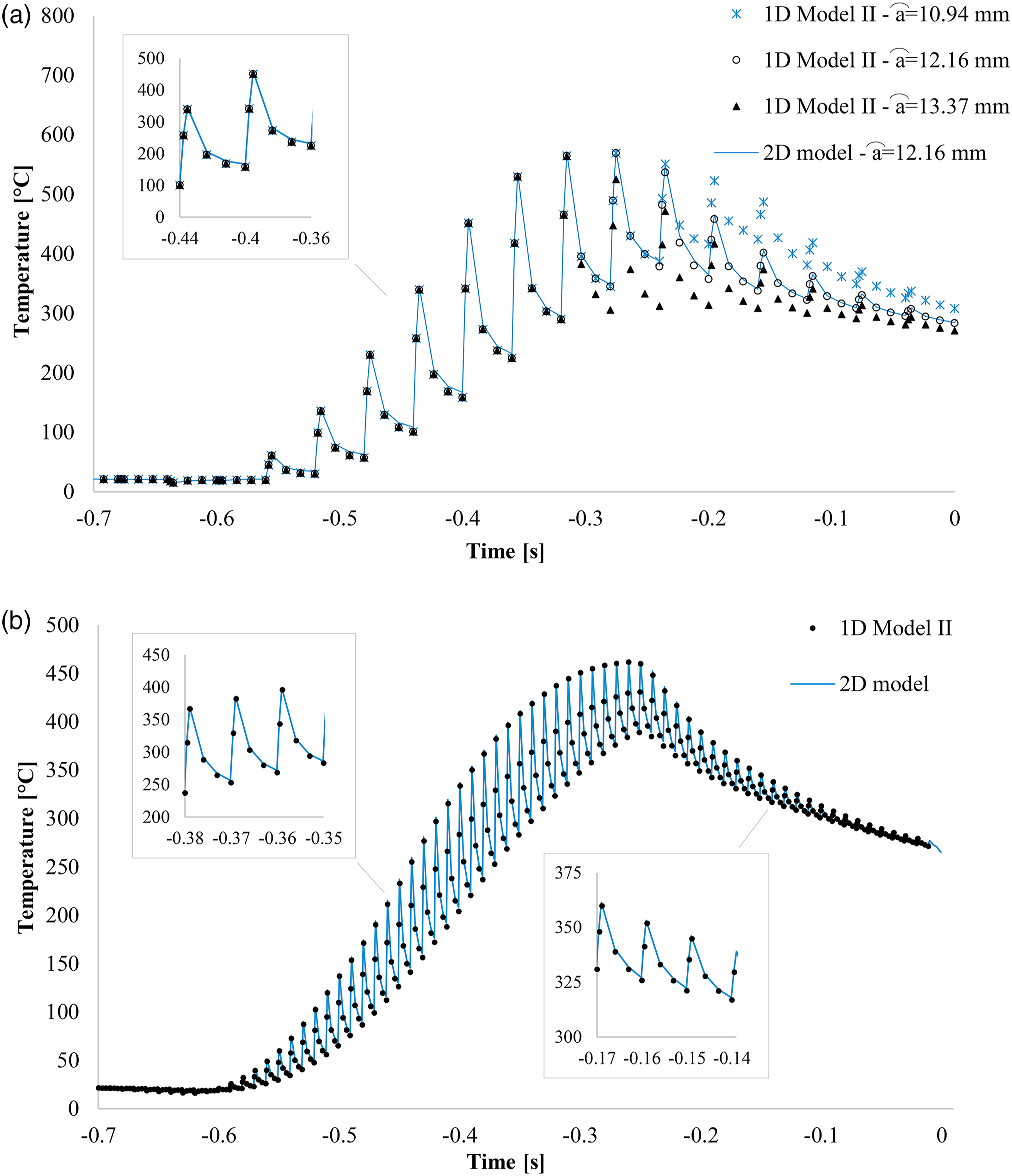

Model II is in good agreement with the 2D model with an average error of 3°C and maximum of 12°C. Similarly to Model I, the deviations are attributed to the exclusion of longitudinal heat conduction as well as the 2D domain of the body in contact, the roller in this case. Errors are also introduced in this case due to the deformed mesh grid across the roller curved section in the 2D model. In addition, the linear velocity attributed to the elements which belong to this section is a function of their distance from the roller centre, ensuring they feature a common angular velocity as part of the same rotating body. Tow surface elements in the 2D model follow the same trajectory; however, elements towards the inner boundary of the roller feature slightly slower linear velocity. The difference in velocities across the tow and roller thickness influences the thermal field evolution, but this effect is small.

Model III verification

A comparison of temperatures developed across the consolidation zone at 50 mms/s is provided in Figure 11 for different deposited material thicknesses, assuming ambient conditions at the start of each new placement. Profiles across different layer interfaces are examined, as this information is typically useful for bond strength studies. Results of the 1D model have been downsampled to an interval of 0.03 s to facilitate visualisation. The developed temperatures decrease away from the nip point due to convection heat losses to the roller, tool, and environment. Lower values are encountered at deeper material levels, whilst as the thickness increases higher temperatures are developed due to the insulating effect of deposited layers. Predictions for the 4^th and 10^th placement are reported in Figures 12 and 13, respectively, for a range of processing speeds. Five interfaces near the surface are examined for the thick deposited material. The time span of the 30 mm long consolidation region (Table 3) is determined by the processing velocity in each case (Figures 12 and 13). The heat flux inputs used in Model I and Model II for these runs at 25 and 100 mm/s have been calculated similarly to the 50 mm/s case (Figure 5). Higher velocities lead to lower temperatures due to the shorter heating times of the deposited material and tow in the previous irradiation stage. The temperature oscillations created on the tapes surface during irradiation have decayed in this region of the process.

Figure 11.

Predictions in the consolidation zone for consecutive placement assuming ambient initial conditions. Interfaces numbering is relatively to the consolidated material surface. Velocity is 50 mm/s and operation is 100 Hz/1.1 ms. 1D data have been downsampled.

Figure 12.

Predictions in the consolidation zone during the 4th placement at different velocities, assuming ambient initial conditions. Interfaces numbering is relatively to the consolidated material surface. Operation is 100 Hz/1.1 ms. 1D data have been downsampled.

Figure 13.

Predictions in consolidation zone during the 10th placement at different velocities. Interfaces numbering is relatively to the consolidated material surface. Operation is 100 Hz/1.1 ms. 1D data have been downsampled.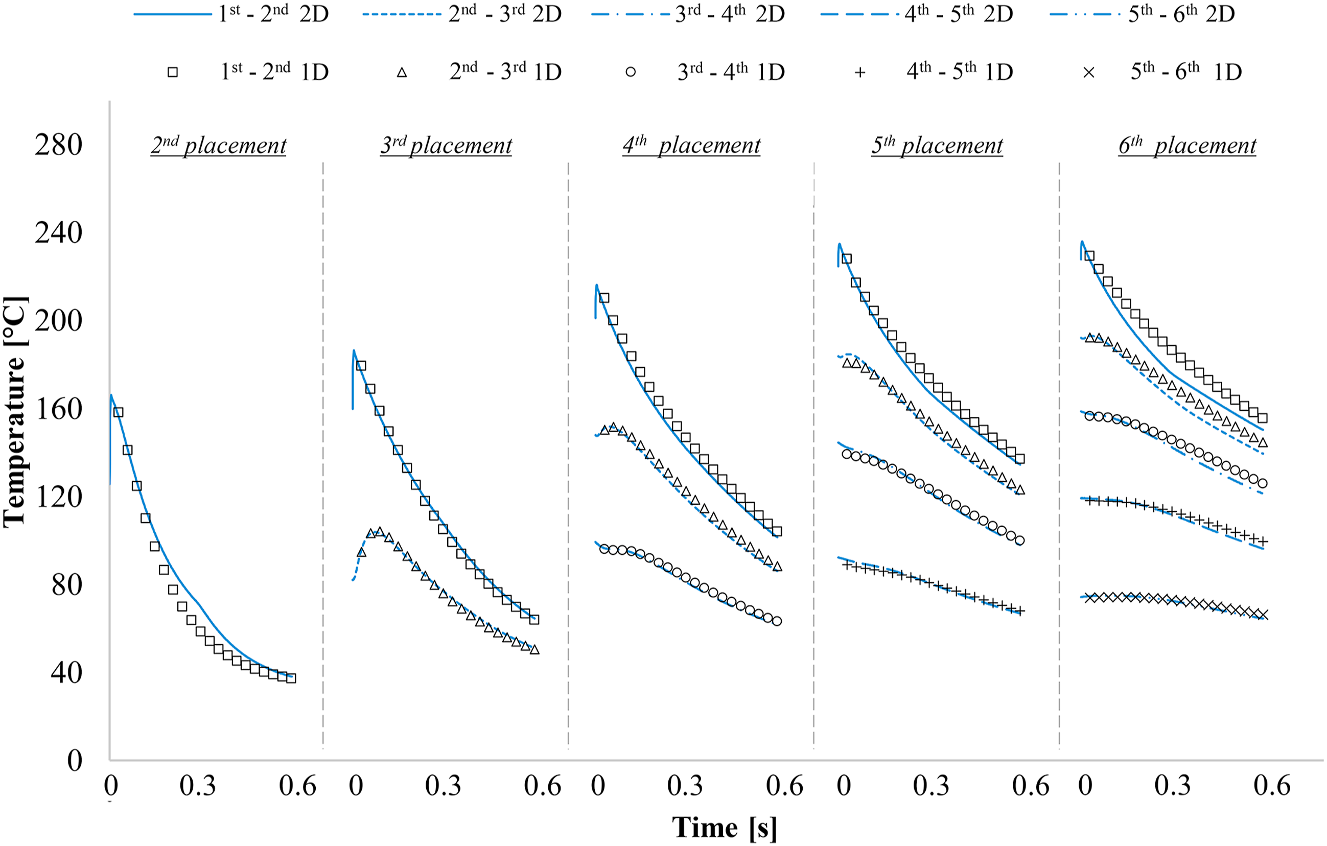

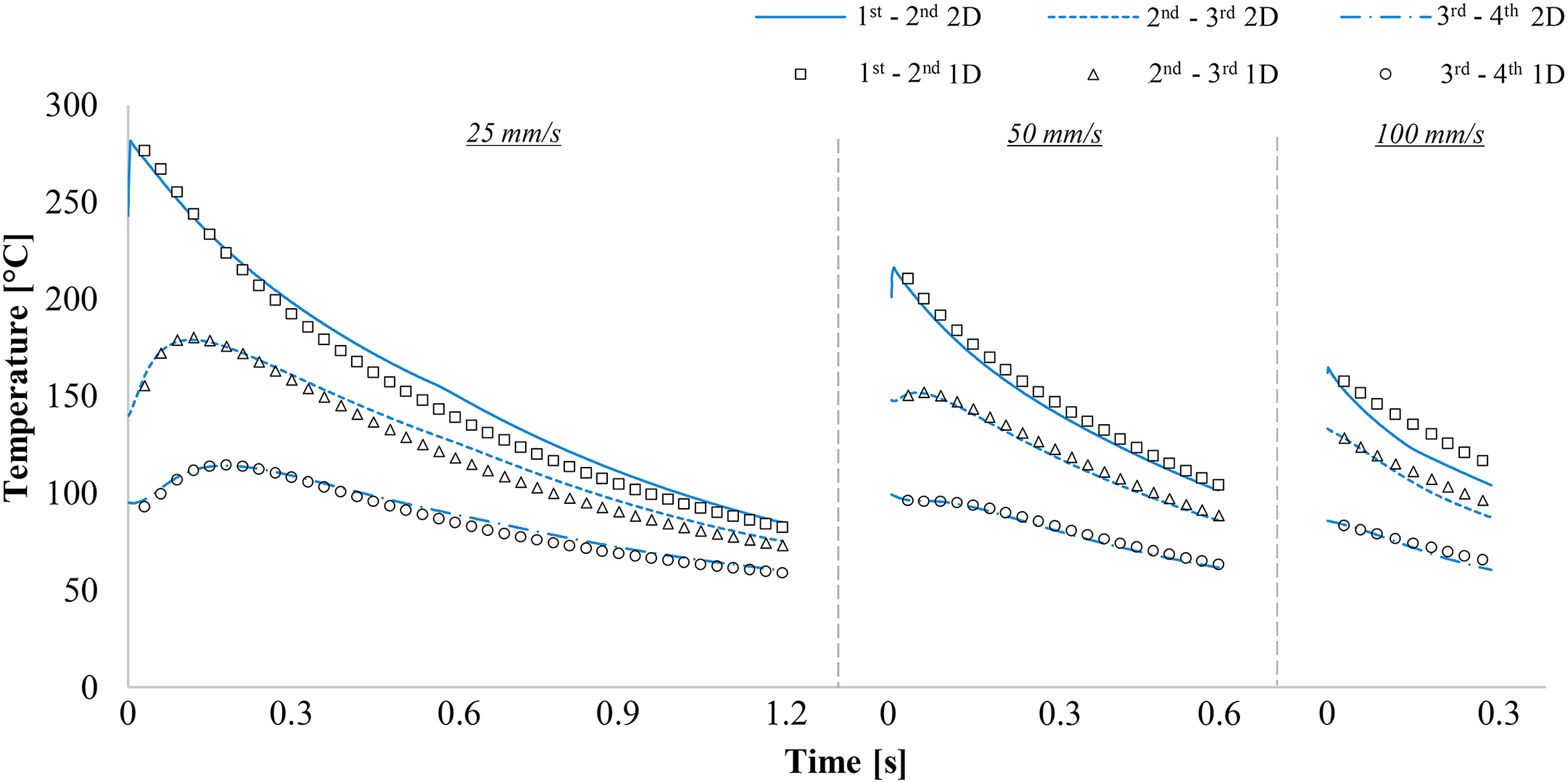
Model III achieves good accuracy with an average error of 4°C and a maximum error of 14°C for all depositions and processing speeds. As in Model I and Model II predictions, these minor errors are attributed to the exclusion of longitudinal heat conduction effects, especially for the highly-conductive tool, and the interaction of the stack with the roller body. As a result, both the tool and the roller representation as 1D bodies introduces errors in the 1D simulation. This effect is more noticeable for interfaces closer to the interface of the stack with the roller. The greatest deviations between the two methodologies in Figures 11–13 are encountered for the 1^st-2^nd layer interface predictions.

Computational efficiency

The floating point operations needed for the solution of the 1D and 2D models are presented in Figure 14, for different deposited material thicknesses and processing conditions. The reported values are calculated based on the CPU time and average computational rate, expressed as floating point operations per second, provided by the finite element software (ANSYS) in the analysis output file. For the 4-core PC (i7-4790) used in this study, the average computational rates were in the 8–12 GFLOPS range.

Figure 14.

Computational effort needed by the two methodologies for different processing scenarios of deposited material thickness, processing rates and pulsing conditions.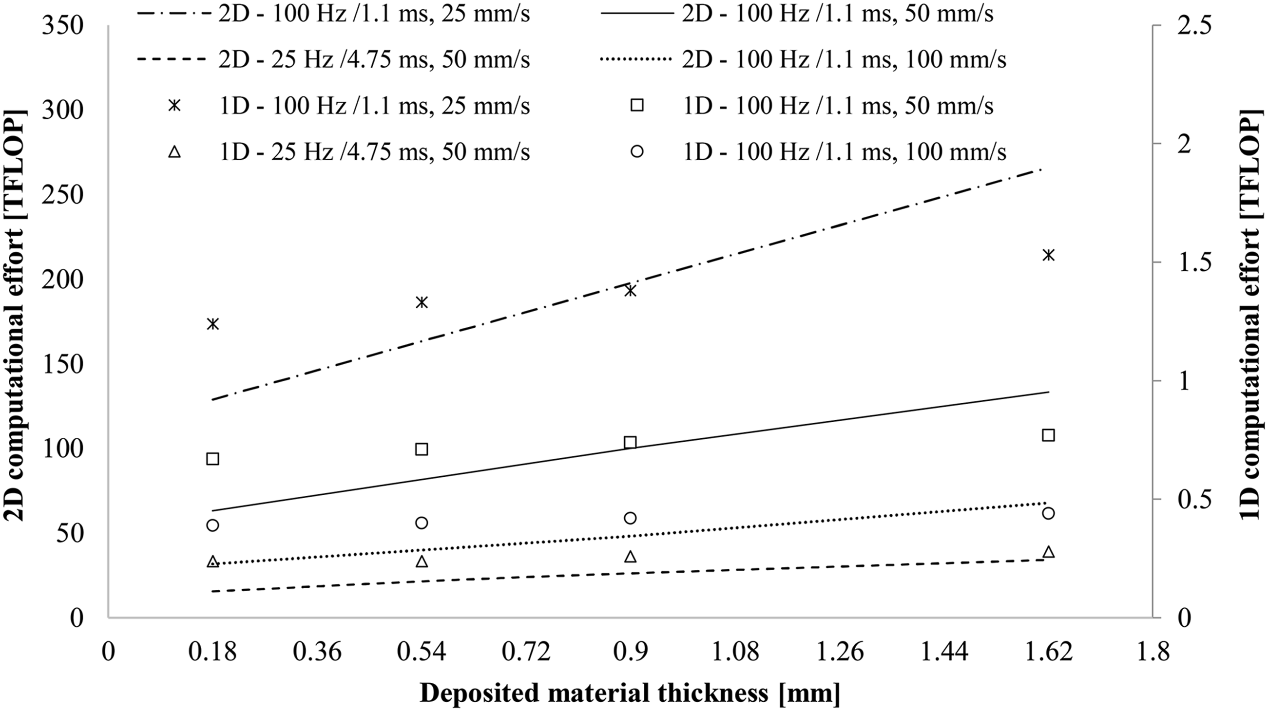

The combined solution of the 1D models requires only 1-2% of the computational effort needed by the 2D analysis for the examined scenarios. The 1D model requires 0.2–1.5 TFLOP operations (20–150 s for the machine used) compared to 16–270 TFLOP (30–450 min for the machine used) of the 2D model. The thickness of the deposited material has a more severe impact on the 2D analysis, with a 100% increase in computational effort between the thinner and thicker composites tested. The 2D solutions require 60 TFLOP and 130 TFLOP (104 and 220 min for the machine used) for a 0.18 and 1.62 mm thick deposited material at 50 mm/s respectively. The floating point operations for the 1D simulation increase only by 25% between these two thicknesses and at 50 mm/s, from 0.67 to 0.77 TFLOP. This difference is caused because each layer introduces a larger number of elements in the 2D analysis due to the 0.09 m long geometry. Computational effort increases proportionally with the pulsing frequency, but decreases with speed for both models due to the changes in the number of steps involved.

The 1D simulation requires significantly lower solution times due to the fewer elements in the analysis. Each submodel represents only a single 1D through-thickness section of the 2D model, thus the solution is carried out for only a small number of elements compared to the 2D version. In addition, the solution for the consolidation zone by Model III uses longer timesteps which contributes to the overall method efficiency. The decoupling of the time discretisation between the irradiation and consolidation zones is specifically advantageous in cases of residual heating effects during consecutive placements. Furthermore, the temperature evolution beyond the roller is critical in the prediction of material phenomena reflecting the final part quality, such as crystallinity and bonding strength development. Very high computational times are required by the 2D model even for the configuration of this study in which the geometry length outside the roller contact part is only 16 mm. Simulating a longer window would add a great number of elements and result in a severe computational penalty. The 1D model accomplishes the simulation of longer processing cycles by extending the analysis time of Model III, with no need of a larger geometry domain. Timesteps of 10 ms were used for Model III in this study; however, their duration can increase gradually away the roller region, subjected to analysis convergence and desirable time resolution. In addition, savings in computation times are expected during the simulation of consecutive layer placements since Model II predictions can be obtained once and used in the modelling of every processing cycle at equivalent conditions, reducing computational effort further.

Experimental validation

The predictions of the 1D simulation are also compared to existing experimental data acquired during the manufacture of AS4/PEEK composites with the ATP configuration examined in this study.²⁵ In work reported previously, thermocouples were mounted on the surface of the deposited material during the 4^th ply deposition at 50 mm/s, operating the flashlamp system at 100 Hz/1.1 ms and 25 Hz/4.75 ms.²⁵ The comparison between 1D model and experiment is illustrated in Figure 15. The 1D simulation of the flashlamp-assisted ATP presents deviations up to 20°C from the temperature measurements across the consolidation zone of the process. The slow response of temperature sensors yielded an average profile of the surface temperature maxima/minima developed in the irradiation phase due to pulsing; however, the mid-level line of model predictions converges satisfactorily to the thermocouple profile. Equivalent conclusions were drawn during the validation of the 2D model,²⁵ which was utilised here as a reference for the 1D simulation development.

Figure 15.

Comparison of 1D simulation predictions against thermocouple data acquired during ATP processing of AS4/PEEK composites²⁵ at 50 mm/s: (a) deposited material surface during the 4th deposition and 25 Hz/4.75 ms operation; (b) deposited material surface during the 4th deposition and 100 Hz/1.1 ms operation.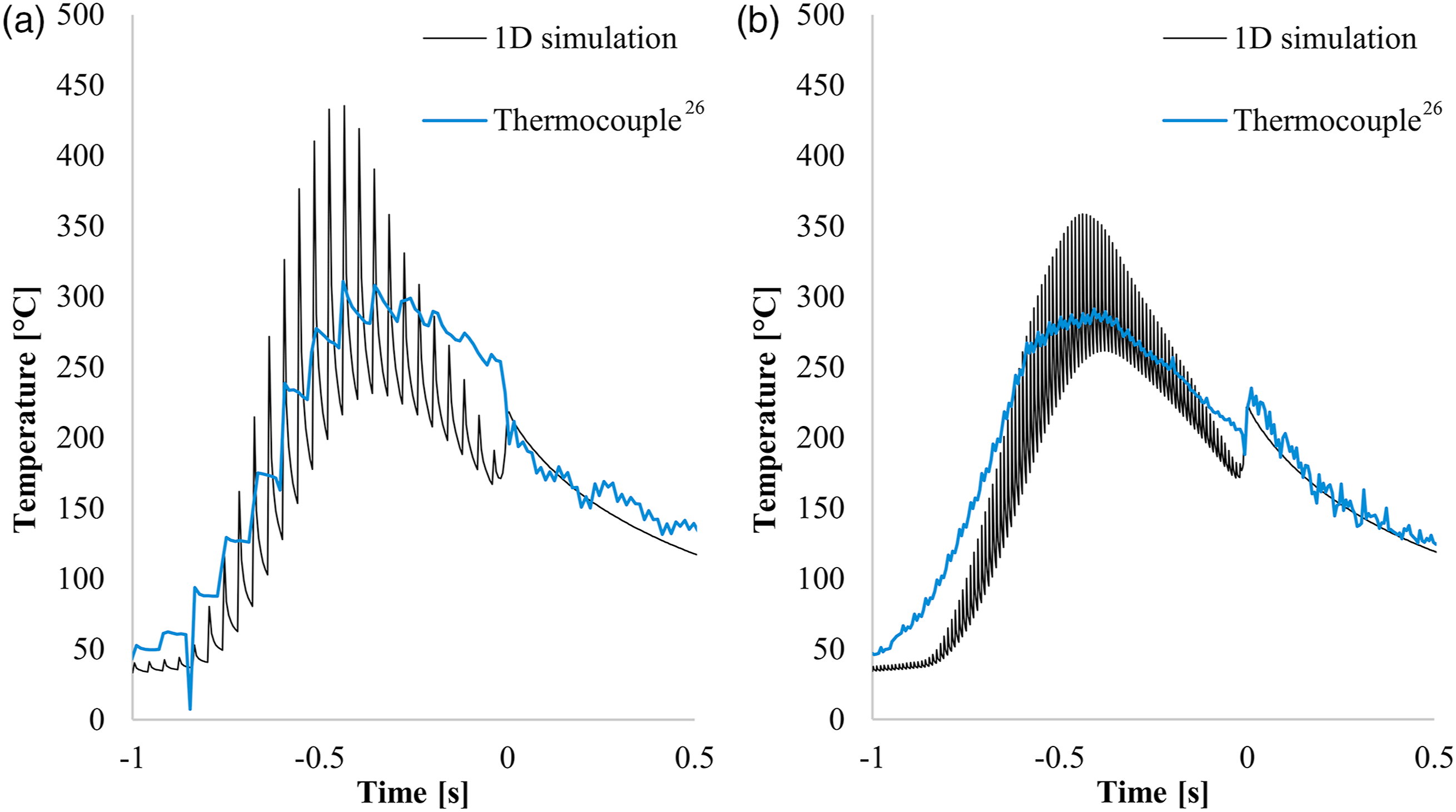

Conclusions

A 1D heat transfer simulation of the flashlamp-assisted ATP was put forward in this study which represents the deposited material, incoming tow and resulting stack as distinct 1D through-thickness models. Appropriate transfer of temperature information ensures field continuity and inclusion of residual heating effects. The accuracy of the model was examined against a validated 2D model of ATP. Deviations up to 14°C were found and attributed mainly to the exclusion of heat conduction in the placement direction in the metallic tool. Equivalent deviations from available experimental data were achieved for the two models. However, the 1D simulation requires only 1-2% of the computational effort compared to the 2D analysis, indicating a significant gain in solution times for a minor trade off in accuracy. This exceptional efficiency is partially attributed to the decoupling of the irradiation and consolidation domains, a highly advantageous feature of the 1D simulation. Longer timesteps can be used across the consolidation and subsequent cooling stage allowing the investigation of temperatures throughout the process more efficiently, compared to existing 2D approaches.

The 1D simulation presented here can be readily integrated in process models of ATP, coupled with material phenomena models, aiming to optimise the process to meet production and quality criteria. The minimisation of processing time, maximisation of bonding strength and control of crystallinity levels as well as the suppression of thermal degradation effects are crucial in the direction of manufacturing high-quality parts at appealing production rates. The accuracy and computation speed of the 1D model enables the investigation of a wide range of process parameters and materials in a feasible timeframe, whilst the ability to simulate pulsed sources ensures that different improvement routes can be explored to achieve the desired results. In addition, large data sets produced by a high number of model runs can be the basis of training AI approaches, as well as of stochastic simulation.

Footnotes

Acknowledgements

This work was supported by the Engineering and Physical Sciences Research Council through the EPSRC Centre for Doctoral Training in Composites Manufacture [grant number EP/L015102/1]. Data underlying this study can be accessed through the Cranfield University repository at .

Declaration of conflicting interests

The author(s) declared no potential conflicts of interest with respect to the research, authorship, and/or publication of this article.

Funding

The author(s) declared the following potential conflicts of interest with respect to the research, authorship, and/or publication of this article: Engineering and Physical Sciences Research Council (EP/L015102/1).

ORCID iDs

Anastasios Danezis

Alex Skordos

References

Pitchumani

Ranganathan

Don

, et al. Analysis of transport phenomena governing interfacial bonding and void dynamics during thermoplastic tow-placement. Int J Heat Mass Transf 1996; 39(9): 1883–1897.

Pistor

Güçeri

. Crystallinity of on-line consolidated thermoplastic composites. J Compos Mater 1999; 33(4): 306–324.

Tierney

Gillespie

Jr . Crystallization kinetics behavior of PEEK based composites exposed to high heating and cooling rates. Compos A Appl Sci Manuf 2004; 35(5): 547–558.

Rosselli

Santare

Güçeri

. Effects of processing on laser assisted thermoplastic tape consolidation. Compos A Appl Sci Manuf 1997; 28(12): 1023–1033.

Khan

Mitschang

Schledjewski

. Parametric study on processing parameters and resulting part quality through thermoplastic tape placement process. J Compos Mater 2013; 47(4): 485–499.

Stokes-Griffin

Compston

. The effect of processing temperature and placement rate on the short beam strength of carbon fibre–PEEK manufactured using a laser tape placement process. Compos A Appl Sci Manuf 2015; 78: 274–283.

Khan

Mitschang

Schledjewski

. Identification of some optimal parameters to achieve higher laminate quality through tape placement process. Adv Polym Technol 2010; 29(2): 98–111.

Yassin

Hojjati

. Processing of thermoplastic matrix composites through automated fiber placement and tape laying methods: a review. J Thermoplast Compos Mater 2017; 31(12): 1676–1725.

Schledjewski

Latrille

. Processing of unidirectional fiber reinforced tapes—fundamentals on the way to a process simulation tool (ProSimFRT). Compos Sci Technol 2003; 63(14): 2111–2118.

10.

Toso

Ermanni

Poulikakos

. Thermal phenomena in fiber-reinforced thermoplastic tape winding process: computational simulations and experimental validations. J Compos Mater 2004; 38(2): 107–135.

11.

Chinesta

Leygue

Bognet

, et al. First steps towards an advanced simulation of composites manufacturing by automated tape placement. Int J Mater Form 2014; 7(1): 81–92.

12.

Lichtinger

Hörmann

Stelzl

, et al. The effects of heat input on adjacent paths during automated fibre placement. Composites A Appl Sci Manuf 2015; 68: 387–397.

13.

Chern

Moon

Howell

. On-line processing of unidirectional fiber composites using radiative heating: I. model. J Compos Mater 2002; 36(16): 1905–1934.

14.

Hörmann

Stelzl

Lichtinger

, et al. On the numerical prediction of radiative heat transfer for thermoset automated fiber placement. Composites A Appl Sci Manuf 2014; 67: 282–288.

15.

Beyeler

Güçeri

. Thermal analysis of laser-assisted thermoplastic– matrix composite tape consolidation. J Heat Transfer 1988; 110(2): 424–430.

16.

Sonmez

Hahn

. Modeling of heat transfer and crystallization in thermoplastic composite tape placement process. J Thermoplast Compos Mater 1997; 10(3): 198–240.

17.

Sarrazin

Springer

. Thermochemical and mechanical aspects of composite tape laying. J Compos Mater 1995; 29(14): 1908–1943.

18.

Mantell

Springer

. Manufacturing process models for thermoplastic composites. J Compos Mater 1992; 26(16): 2348–2377.

19.

Ghasemi Nejhad

Cope

Güceri

. Thermal analysis of in-situ thermoplastic composite tape laying. J Thermoplast Compos Mater 1991; 4: 20–45.

20.

Agarwal

Guçeri

Mccullough

, et al. Thermal characterization of the laser-assisted consolidation process. J Thermoplast Compos Mater 1992; 5(2): 115–135.

21.

Grove

. Thermal modelling of tape laying with continuous carbon fibre- reinforced thermoplastic. Composites 1988; 19(5): 367–375.

22.

Stokes-Griffin

Compston

. A combined optical-thermal model for near-infrared laser heating of thermoplastic composites in an automated tape placement process. Compos A Appl Sci Manuf 2015; 75: 104–115.

23.

Kim

Lee

. A study on heat transfer during thermoplastic composite tape lay-up process. Exp Therm Fluid Sci 1996; 13(4): 408–418.

24.

Maurer

Mitschang

. Laser-powered tape placement process – simulation and optimization. Manuf Polym Compos Sci 2015; 1(3): 129–137.

25.

Danezis

Williams

Edwards

, et al. Heat transfer modelling of flashlamp heating for automated tape placement of thermoplastic composites. Compos A Appl Sci Manuf 2021; 145: 106381.

26.

Tierney

Gillespie

. Modeling of heat transfer and void dynamics for the thermoplastic composite tow-placement process. J Compos Mater 2003; 37(19): 1745–1768.

27.

Dai

. GF/PP tape winding with on-line consolidation. J Reinf Plast Compos 2002; 21(1): 71–90.

28.

Weiler

Emonts

Wollenburg

, et al. Transient thermal analysis of laser-assisted thermoplastic tape placement at high process speeds by use of analytical solutions. J Thermoplast Compos Mater 2017; 31(3): 311–338.

29.

Yang

. Dynamic finite element simulation and transient temperature field analysis in thermoplastic composite tape lay-up process. J Thermoplast Compos Mater 2015; 28(4): 558–573.

30.

Schaefer

Gierszewski

Kollmannsberger

, et al. Analysis and improved process response prediction of laser-assisted automated tape placement with PA-6/carbon tapes using design of experiments and numerical simulations. Compos A Appl Sci Manuf 2017; 96: 137–146.

31.

Heider

Piovoso

Gillespie

. A neural network model-based open-loop optimization for the automated thermoplastic composite tow-placement system. Compos A Appl Sci Manuf 2003; 34(8): 791–799.

32.

Humm3™-intelligent heat for automated fibre placement (AFP). www.heraeus.com, 2022.

33.

Kim

Sung Jung

June Kim

, et al. Inverse estimation of thermophysical properties for anisotropic composite. Exp Therm Fluid Sci 2003; 27: 697–704.

34.

Cogswell

. Thermoplastic aromatic polymer composites: a study of the structure, processing, and properties of carbon fibre reinforced polyetheretherketone and related materials. Oxford: Butterworth Heinemann, 1992.

35.

Ansys® mechanical enterprise, release 2021 R1, help system, thermal analysis guide. Canonsburg, Pennsylvania, USA: ANSYS Inc, 2022.

One-dimensional approximation of heat transfer in flashlamp-assisted automated tape placement

Abstract

Keywords

Introduction

Model formulation

Model I–deposited material

Model II–incoming tow

Model III–consolidation zone

Integration of the three 1D models

Methodology

Results and discussion

Model I verification

Model II verification

Model III verification

Computational efficiency

Experimental validation

Conclusions

Footnotes

Acknowledgements

Declaration of conflicting interests

Funding

ORCID iDs

References