
Abstract
The optimisation and control of automated tape placement (ATP) requires fast analysis tools able to utilise process data for predictions and monitoring. In this study, a strategy for in-process estimation of nip point temperatures is proposed. The method is based on a combination of two one-dimensional analytical solutions of heat transfer in ATP using temperature data measured on the tool surface, combined with an inverse solution for the estimation of power delivered by the heating device on the composite surface. The performance of the method is examined against a validated finite element model. Approximations of nip point temperature show good correlation for different tool materials, with an average error of 15°C and a maximum of 50°C which is satisfactory for the processing of high-temperature thermoplastic materials. The analytical scheme offers real-time estimations of the nip point temperature with the potential to be used for process control of ATP.
Keywords
Introduction
The increasing demand for large composite structures has driven forward the automation of manufacturing methods to overcome low production rates and the variability associated with manual techniques. Automated tape placement (ATP) is an advanced manufacturing process which deploys robotic deposition of tapes onto a tool, building the part in an additive fashion. ATP has gained significant industrial and research interest 1 due to its potential to operate as a single-step process for thermoplastic composites. However, quality on a par with conventional methods is yet to be achieved due to process complexity. Further advancements on the analysis, process monitoring and industrial equipment fronts are necessary to enable the wider adoption of automated methods such as ATP.
Design and optimisation of ATP is a challenging task due to the high number of manufacturing parameters influencing the process and the non-linear heat transfer phenomena involved. Part quality depends strongly on the selection of these parameters, with the influence of temperature history on bond strength development, crystallinity, void content, and thermal degradation playing a critical role.2–5 These effects have been investigated using heat transfer simulation of ATP, mainly by solving the boundary value problem using numerical methods. 6 Three-dimensional models have been developed,7-9 but in most cases the domain is reduced to two dimensions assuming uniform heating across the tape width.10–16 Further simplifications are made by neglecting the heat diffusion in the placement direction based on the dominance of heat transfer due to advection as indicated by the Peclet number.17,18 In some cases, exo/endo-thermic effects have been included in the analysis,9–12 while in other cases these have been assumed to be negligible.13–18 Analytical solutions for the simplified one-dimensional heat transfer problem have been derived.19–21 In some cases, thermal simulations coupled with material reaction models have been used for process optimisation.22–24 Surrogate models as well as neural networks and machine learning have been deployed, trained by offline simulation25–27 or post manufacture data expanded using virtual sample generation methods. 28 Neural networks have been combined with thermal imaging for on-line training and feedback control. 29
Use of predictive simulation yields results corresponding to ideal process conditions and material properties. Producing zero defect parts with ATP can be facilitated by in-process monitoring to incorporate variations in material behaviour and conditions in process optimisation and control. In the context of ATP, thermography and laser-vision have been used to identify placement and steering defects.30–33 Optical fibre Bragg grating sensors have also been used to monitor the temperature and strain during placement. 34 These strategies serve an on-line inspection role rather than acting as part of a process control system. Utilisation of thermal measurements in conjunction with inverse methods to identify parameters of the process on-line and project their influence on the product has been put forward in the context of the curing stage of thermosetting composites manufacture.35,36 Such a development is not currently available for ATP, mainly due to the difficulty of acquiring accurate temperature measurements on the material as it is processed. Thermal imaging is typically used as it allows remote continuous measurements during placement.30,31 However, the process nip point and bonding zone are typically out of sight under the compaction roller, and the viewing angle varies with the robot head movements or is limited over convex geometries. Closed-loop control systems based on thermal imaging measure and control temperatures away from the nip point for these reasons; however, significant temperature drop can occur until the material arrives at the nip point due to roller shadowing.14,17 Embedding sensors in, or in contact with, the moving material is only possible in experimental setups, but not in a production environment due to the additive nature of the process. The concept of a closed-loop control system using thermocouple readings and an approximate process model has been outlined, 19 but its development has not been carried out. Establishing a method for in-process estimation of the temperature at critical locations in the ATP process is a fundamental step in exploiting its automation and high rate potential while meeting product quality requirements.
In this study, a monitoring strategy for ATP of thermoplastic prepregs is put forward based on a combination of 1D heat transfer analytical solutions and temperature data acquired on the tool surface, in contact with the composite substrate, allowing the estimation of nip point temperature in real time. The method integrates an inverse solution to determine the heater power input from the temperature data and enhance the accuracy of nip point estimation. The accuracy of the scheme is assessed against the outputs of a validated 2D finite element model of flashlamp-assisted ATP 17 for a wide range of process rates, number of substrate layers and tool materials. The analytical scheme and inverse solution are also applicable to continuous heating due to the similar bondline temperatures for pulsed and continuous sources of equivalent average power. 17 A virtual processing scenario is studied to showcase the scheme’s ability to identify condition changes and highlight the benefits of ATP process monitoring.
Analytical heat transfer approximation of ATP
The 1D analytical approximation combines two solutions describing the two different regimes of heat transfer in ATP. As the part is built up and the thickness increases, the heat transfer shifts from that of a material slab with finite thickness to a semi-infinite body. The transition between the two behaviours is indicated by the Fourier number,
19
which expresses the ratio between conductive heat transport and power storage, with conductive transport being dominant for thin stacks whilst power storage governing heat conduction at high thickness. The Fourier number is
In tape placement terms, a high Fourier number means that the material thickness is low and/or the process slow enough for a temperature gradient to be established across the thickness direction, whilst a low value implies the deposited material is too thick and/or the process too fast for a significant material depth to be affected by the incoming energy prior to the nip point. The existence of these two heat transfer regimes necessitates two different solutions to approximate conduction effects and a strategy for the transition from one behaviour to the other.
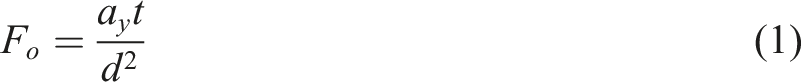
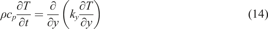
The full ATP heat transfer problem can be reduced to 2D by assuming uniform heating across the tape width and no edge effects.10–16 In a Eulerian frame attached to the moving placement head, the 2D energy balance coupled with Fourier’s heat conduction law is:

Further simplification of equation (2) can be made as the Peclet number in the placement direction

No material motion takes place in the thickness direction leading to:
The next step of the approximation is to represent the substrate and incoming tow as a single slab which corresponds to the geometry at the nip point section. This material slab is heated at its surface, has a thickness Heat transfer in ATP: (a) 2D representation; (b) simplification of geometry to a single material slab; (c) finite slab behaviour with averaged volumetric heating for Fo>1; (d) semi-infinite body behaviour under surface heating at greater thickness (Fo<1).
Finite slab approximation
For the finite slab behaviour, assuming the material has a uniform temperature at the start of the irradiation zone and at the nip point,

Equation (5) can be integrated in the
Equation (6) links the material temperature at the start of the irradiation and at the process nip point. Although the entry temperature in ATP is typically ambient and thus uniform, this is not true for the nip point section where steep through-thickness profiles are developed as a result of the energy delivered on the surface of the material and the low transverse thermal conductivity of the material.
17
To account for this, the temperature profile at the nip point location is assumed to have a bilinear shape as shown in Figure 1(c). The temperature of the first ply is assumed to be constant

In the approximation expressed by equations (5)–(7), the energy balance operates using the average temperature of the deposited material through the thickness, while surface heat flux becomes part of the heat rate term

The latent heat term
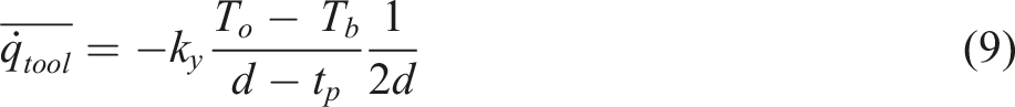
The average power losses per unit volume of material due to contact with the tool can be approximated as the average heat transfer by conduction between the lower surface of the first ply and the lower surface of the material slab, assuming a linear increase of
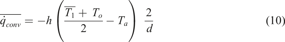
Similarly, the power losses to air per unit volume due to convection can be approximated as:
The average volumetric power input due to radiative heating is:
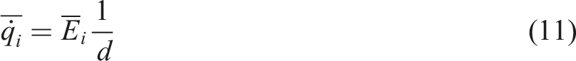
Combining equations (9)–(11), the total heat rate per unit volume of material is:
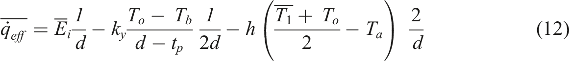
Combination of equations (6), (7) and (12) yields:
Semi-infinite body approximation
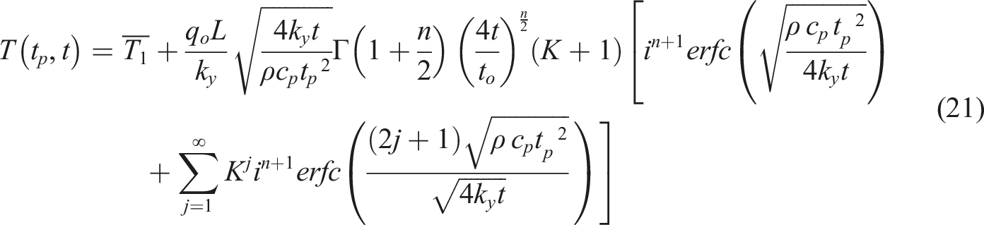
As the substrate thickness increases the heat transfer phenomena approach the behaviour of a semi-infinite solid with a heat flux
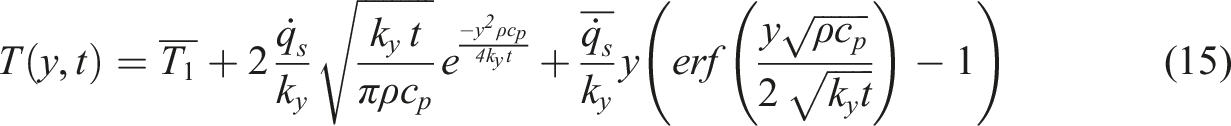
Here
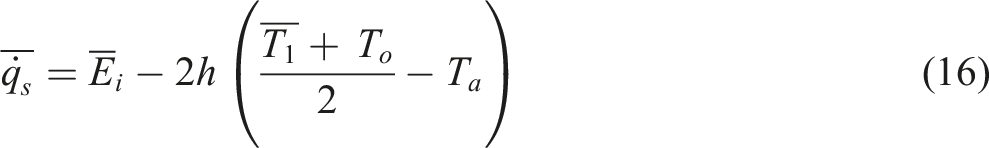
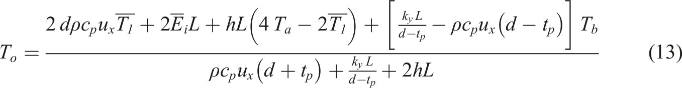
Combining equations (15), and (16) for the nip point position
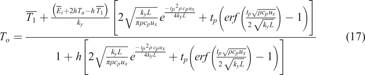
Transition between behaviours
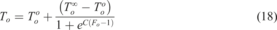
The approximations represented by equations (13) and (17) are effective for the case of thin and thick composite substrates respectively. The transition between the two behaviours is governed by the instantaneous Fourier number (equation (1)). Switching between these two behaviours can be done predictively by using the Fourier number and setting a threshold value of 1 for the transition. To ensure the transition in behaviour does not cause a discontinuity, a smooth step using the logistic function is selected between the two solutions:
Inverse estimation of heater power input
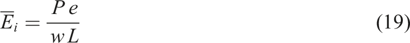
A value of average irradiance
Using the same transformation and assumptions as those utilised to obtain equation (14) but for the case of the tool incorporated in the model as a semi-infinite body, the temperature at the interface between the composite and the tool, which coincides with the sensor location during the second deposition at
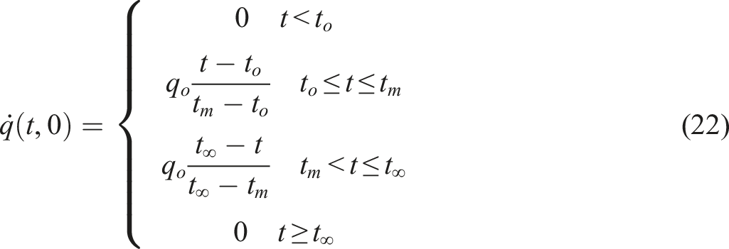
In general, the irradiance acting on the tapes follows an asymmetric bell shape.14,17 This can be approximated by a time-varying triangular profile as illustrated in Figure 2, expressed by: Schematic of the triangular irradiance with the function segments expressed by equation (22), and the configuration of the 1D solution deployed for the inverse scheme.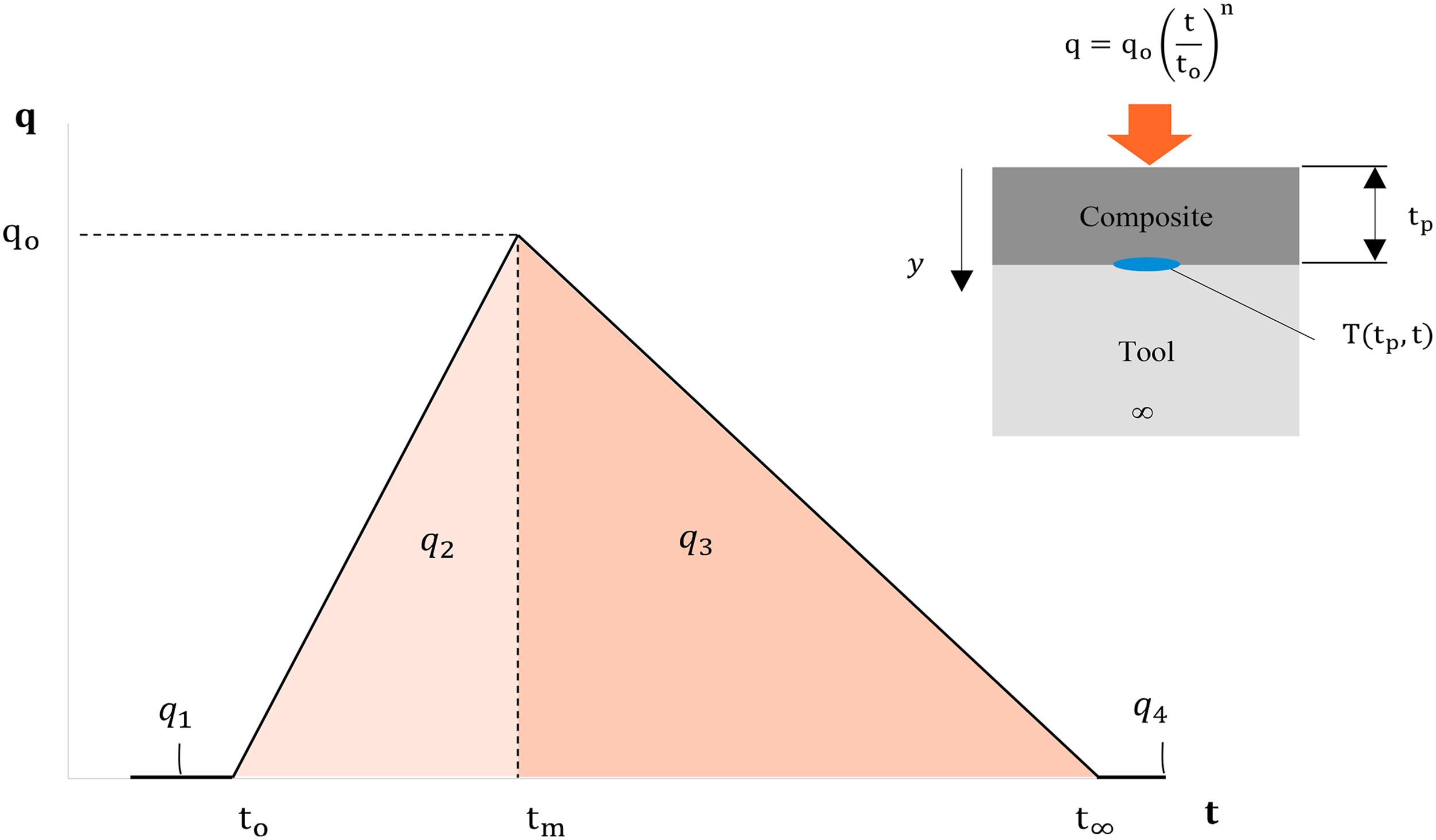

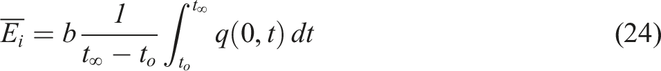
The average irradiance acting on the composites inside the ATP cavity is:
The irradiance acting on the tapes is expected to scale linearly with the total power of the heating source whilst changes to the processing rate only rescale the time variable of the distribution. In addition, the irradiance distribution is independent of the inlet temperature and substrate thickness. Therefore, the distribution retrieved with this method corresponds to a placement path and can be used during future depositions across the same path regardless of the changes to these parameters. This method cannot be applied during the first ply deposition as the tool optical properties are different from the tapes, leading to an irradiance distribution not applicable to subsequent processing cycles with a composite substrate.
Strategy for in-process nip point temperature estimation
An overview of the proposed strategy for in-process estimation of nip point temperatures in ATP is illustrated in Figure 3. The manufacturing of the composite part takes place on a tool with a number of sensors strategically placed. The sensors record and feed the controller continuously. Each sensor captures the tool surface temperature Overview of the strategy for in-process nip point temperature estimation in ATP and utilisation of the modelling estimates for process control.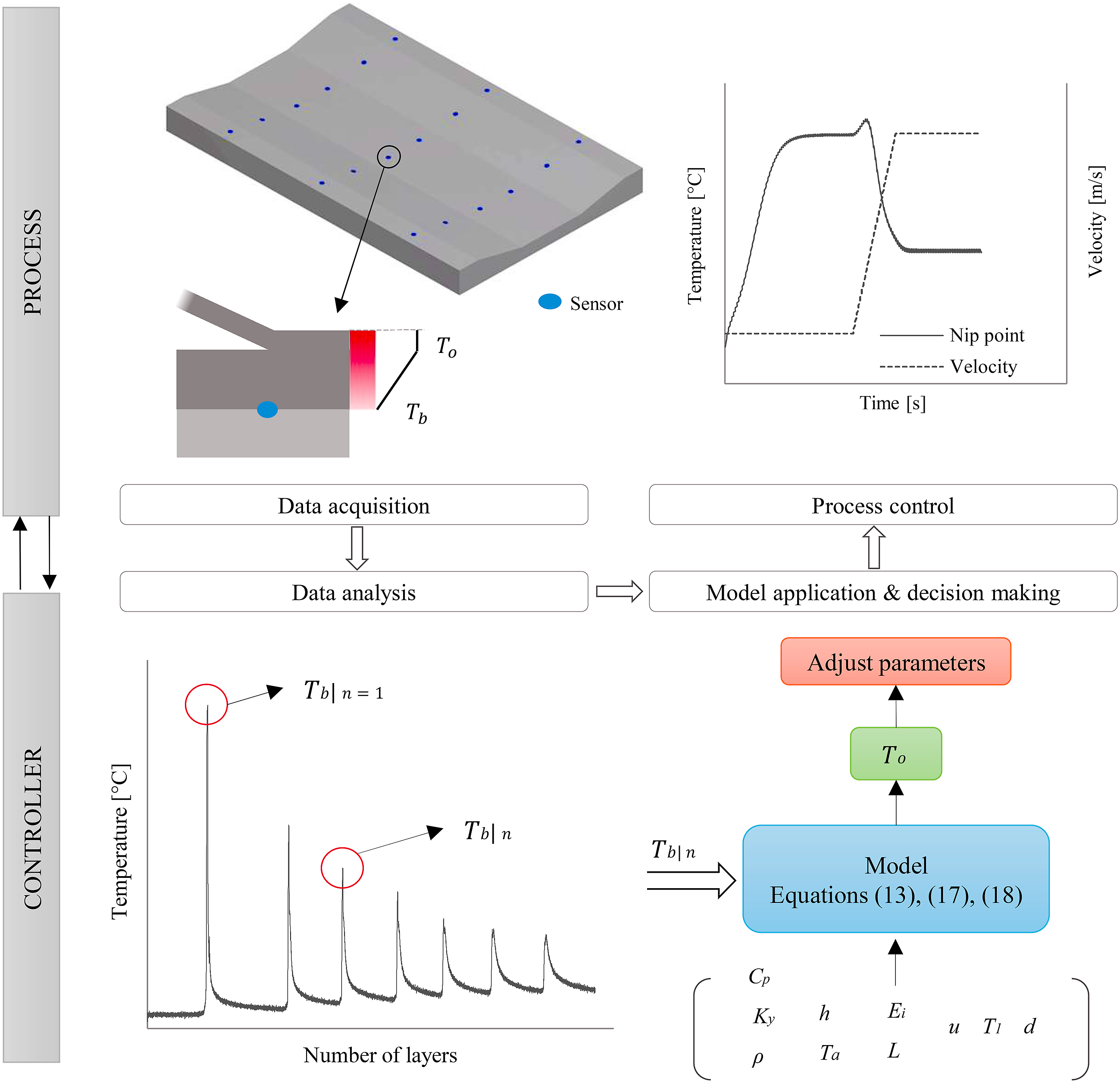
Knowledge of the nip point temperature obtained using the approach presented here can allow adjustment of the process conditions through on-line control to maintain its value within an optimal envelope. The processing velocity and heat source power can be adjusted according to the sensitivity of the nip point temperature to these variables. This strategy allows conditions to be adapted as the process progresses and the build-up of thickness alters the heat transfer conditions. Furthermore, potential variability resulting in changes in heat transfer conditions around the part manufactured can be addressed.
Methodology
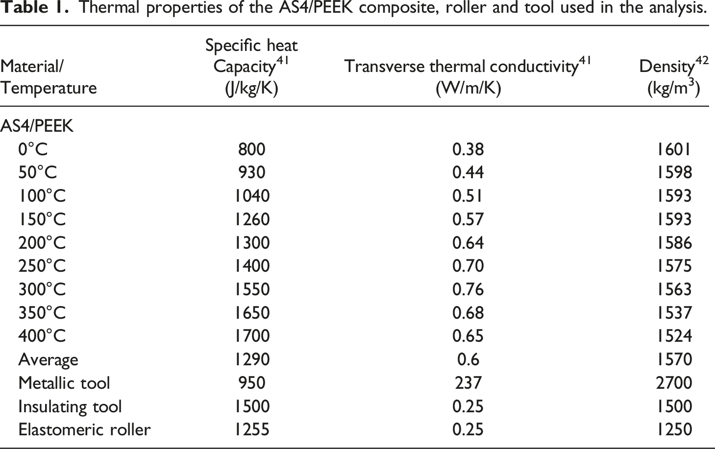
Thermal properties of the AS4/PEEK composite, roller and tool used in the analysis.
Overview of the analytical and FE model comparison.
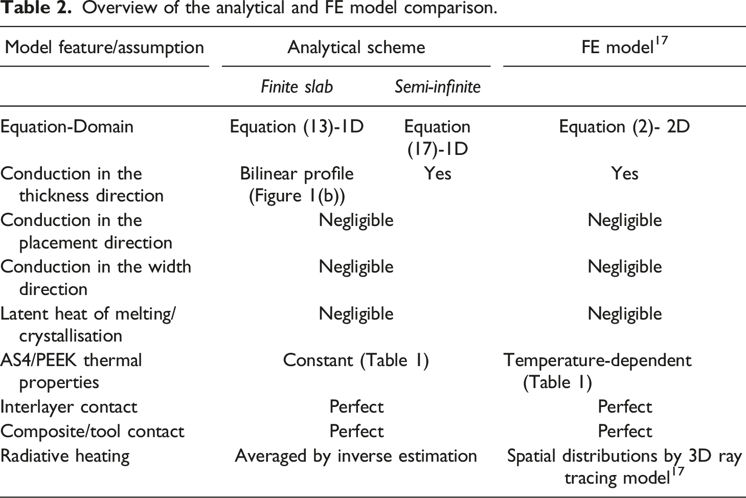
Although the simulation data were generated for a flashlamp-assisted ATP process, similar behaviour is expected under continuous heating. Previous work has shown that the bondline temperatures are similar for pulsing and continuous sources of equivalent average power. 17 In addition, the effect of pulsing on the surface is diminished at one ply depth. As a result, the performance assessment of the analytical scheme and application of the inverse solution carried out for a pulsed source here can be extended to continuous sources.
Results and discussion
Inverse estimation of irradiance
The temperature profiles on the tool surface predicted by the FE model during the second ply deposition at 100 mm/s are plotted in Figure 4 for metallic and insulating tooling. The profiles correspond to the temperature history of a material point which moves across the 110 mm long analysis frame at the interface between the first ply and the tool. The point enters the irradiation region at 0.2 s at a temperature of 20°C and reaches the nip point at 0.8 s after which a secondary temperature peak occurs due to the additional energy the substrate gains in this case when it comes into contact with the hot incoming tow underneath the roller (0.8–0.94 s). Significantly higher temperatures develop on the surface of the insulating tool during deposition due to its low conductivity which reduces the dissipation of energy. In order to simulate typical noisy temperature sensor data, a Gaussian noise of zero mean value was added to the FE profiles (Figure 4). The standard deviation was set at 2°C for the metallic tool and 20°C for the insulating one, representing approximately 10% of the maximum temperature reached in each case. Temperature profiles (FE model) on the tool surface during the 2nd ply deposition at 100 mm/s used for the inverse calculation of irradiance on the substrate surface, before and after the addition of Gaussian noise. Identical independent normally distributed increments with a standard deviation of 2°C for the metallic tool and 20°C for the insulating tool were used to generate the noise superimposed on the FE results.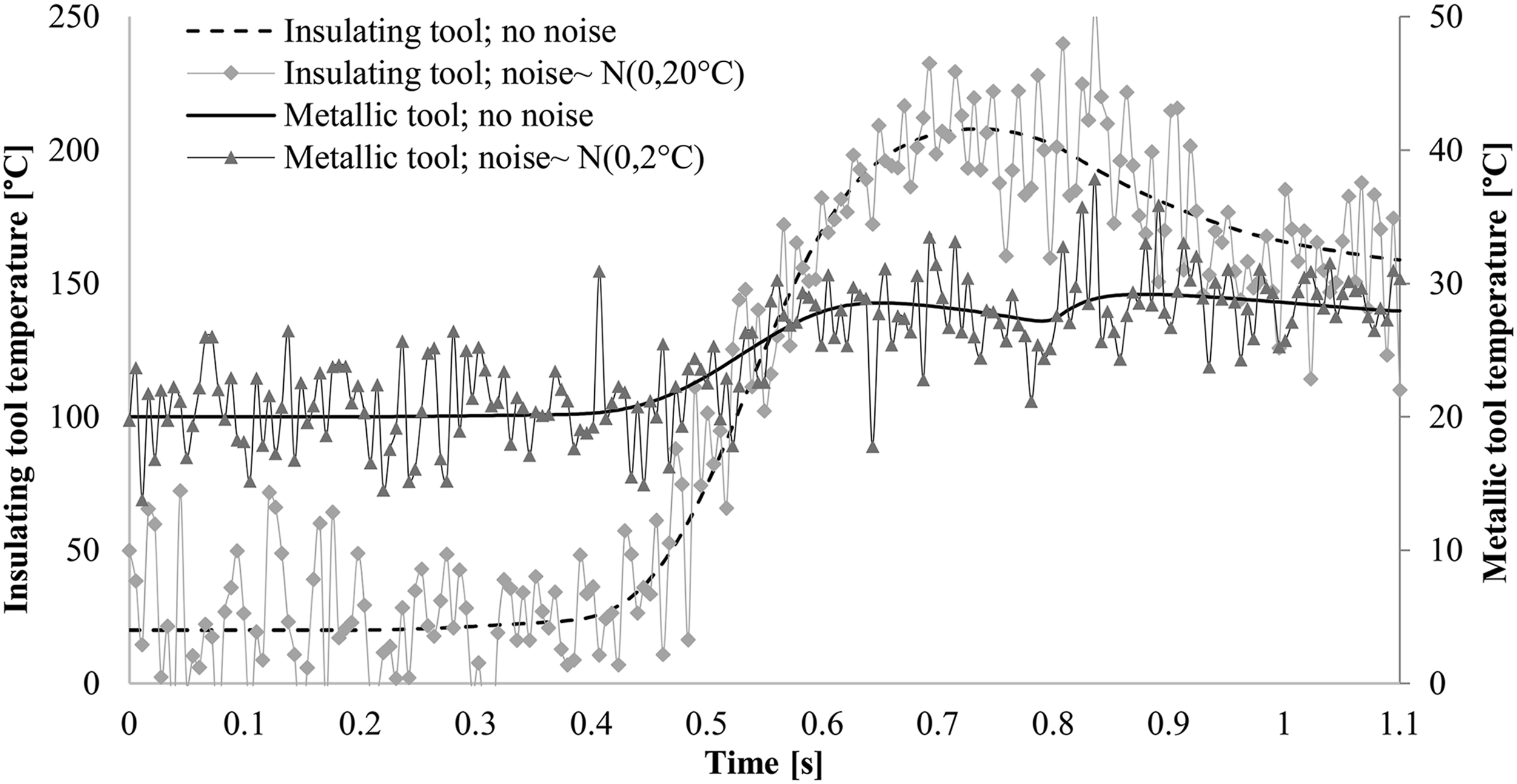
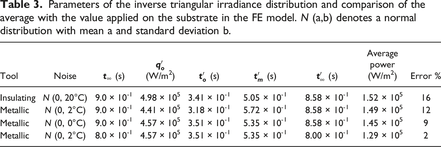
The inverse scheme was applied to determine the irradiance input (
Parameters of the inverse triangular irradiance distribution and comparison of the average with the value applied on the substrate in the FE model. N (a,b) denotes a normal distribution with mean a and standard deviation b.
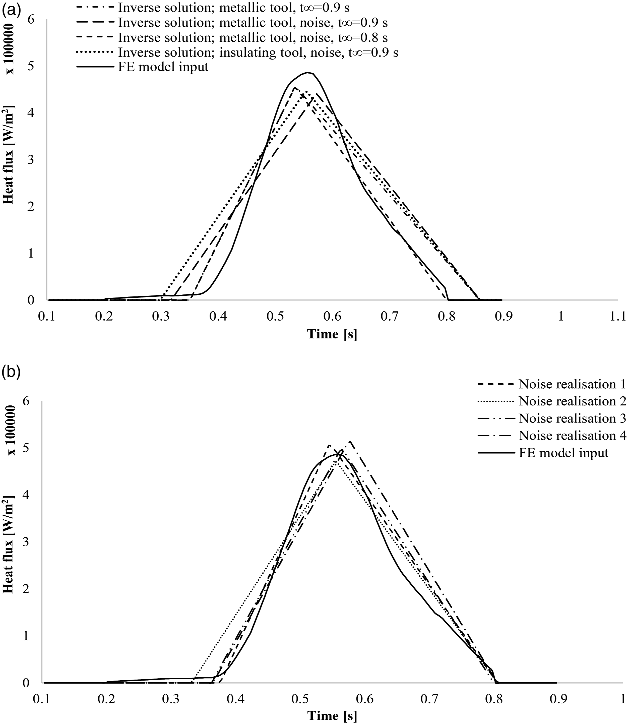
Inverse calculation of irradiance distribution: (a) profiles recovered and the profile applied on the FE model; (b) estimation for different noise realisations for the case of metallic tool, noise of 2°C standard deviation and t∞ fixed at 0.8 s.
Overall, the inverse solution yields satisfactory results even when significant noise is incorporated in the temperature data and sensor position uncertainty exists. The problem of identifying a boundary heat flow based on temperature measured at a depth within the domain is ill-posed. 43 The use of a strong function specification through the triangular profile has a regularising effect on the estimation problem resulting in a robust inversion. Furthermore, the triangular profile is the simplest shape representing the irradiance distribution in ATP and can be expressed in the form of equation (20); and therefore, used in the direct solution of equation (21). The method put forward here obtains an estimate of the irradiance distribution by experimental means with inaccuracy similar to more complicated and time-consuming off-line studies such as optical modelling, whilst also including effects of variability which cannot be considered in off-line computations. The influence of parameters that are either difficult to determine or subject to significant variability, such as the heater efficiency or optical absorptivity, is included in the data captured in real time during the process, and therefore is directly incorporated in the inverse prediction, making the proposed method advantageous compared to off-line predictive strategies.
Nip point temperature determination
Comparison of the FE and analytical predictions of the nip point temperature is presented in Figure 6 for a wide range of process velocities, number of plies and different tool materials, whilst Figure 7 shows a regression plot of the approximate model versus the FE results. The total irradiance used for all analytical calculations corresponds to the case of metallic tooling with 2°C standard deviation noise and Comparison of the FE and analytical model predictions for a range of velocities, number of layers and: (a) metallic tool; (b) insulating tool. Regression plot of the analytical and FE model predictions indicating good agreement between the two data sets.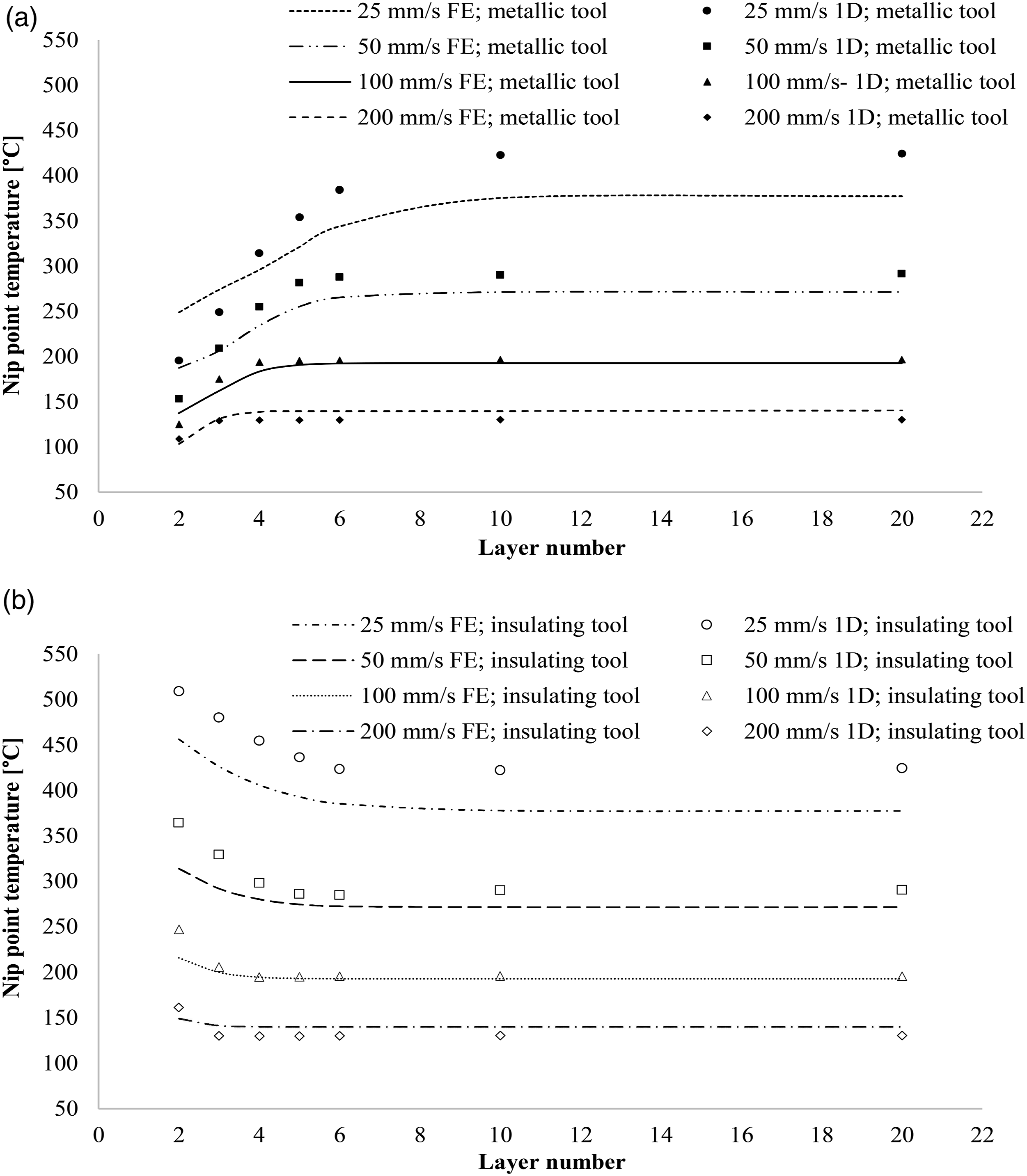
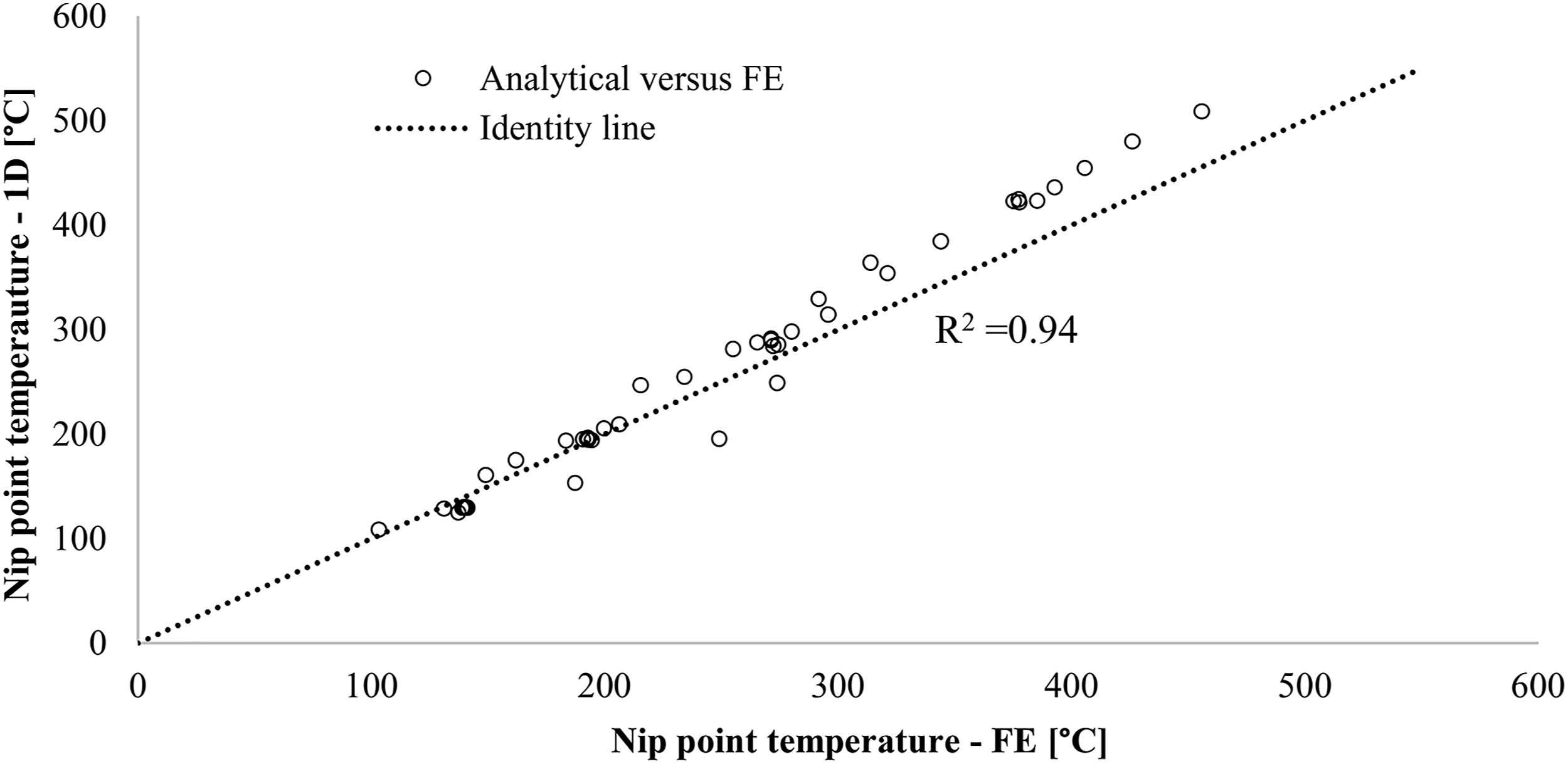
Figure 6 shows that the nip point temperature decreases with increasing rate whilst for a given velocity the temperature evolves as the process progresses in a way which depends on the tool material. For the conductive metallic tool (Figure 6(a)), the nip point temperature increases for several layers at the start of the process until it reaches a plateau at which subsequent layer depositions result in similar values. This is caused by the low conductivity of the composite, which reduces heat losses to the tool as its thickness increases, resulting in higher temperature near the surface. The influence of conduction losses towards the tool becomes negligible after a number of layers, depending on the placement velocity. In contrast, the nip point temperature for the insulating tool (Figure 6(b)) decreases for several layers until it converges to the same plateau value as for the metallic tool. The nip point temperatures reached at low thickness are significantly higher compared to the case of highly conductive metallic tooling. In this case, the tool acts as a thermal barrier to heat diffusion resulting in higher nip point values. For the given data, the plateau is reached approximately after the fourth ply at 200 mm/s and the 10th ply at 25 mm/s. This plateau indicates the transition of the heat transfer physics to that of a semi-infinite solid for which an increase of thickness or changes in the tooling material properties do not affect the temperature field. This transition coincides with the reduction of the Fourier number below 1; therefore, it can be predicted, and it is taken in account automatically in the approximation through equation (18). As a result, the predictions for the plateau rely on the semi-infinite solution expressed by equation (17). This transition is also reflected in the tool temperature Tool temperature at the nip point section (Tb) given by the FE model used for the analytical calculations.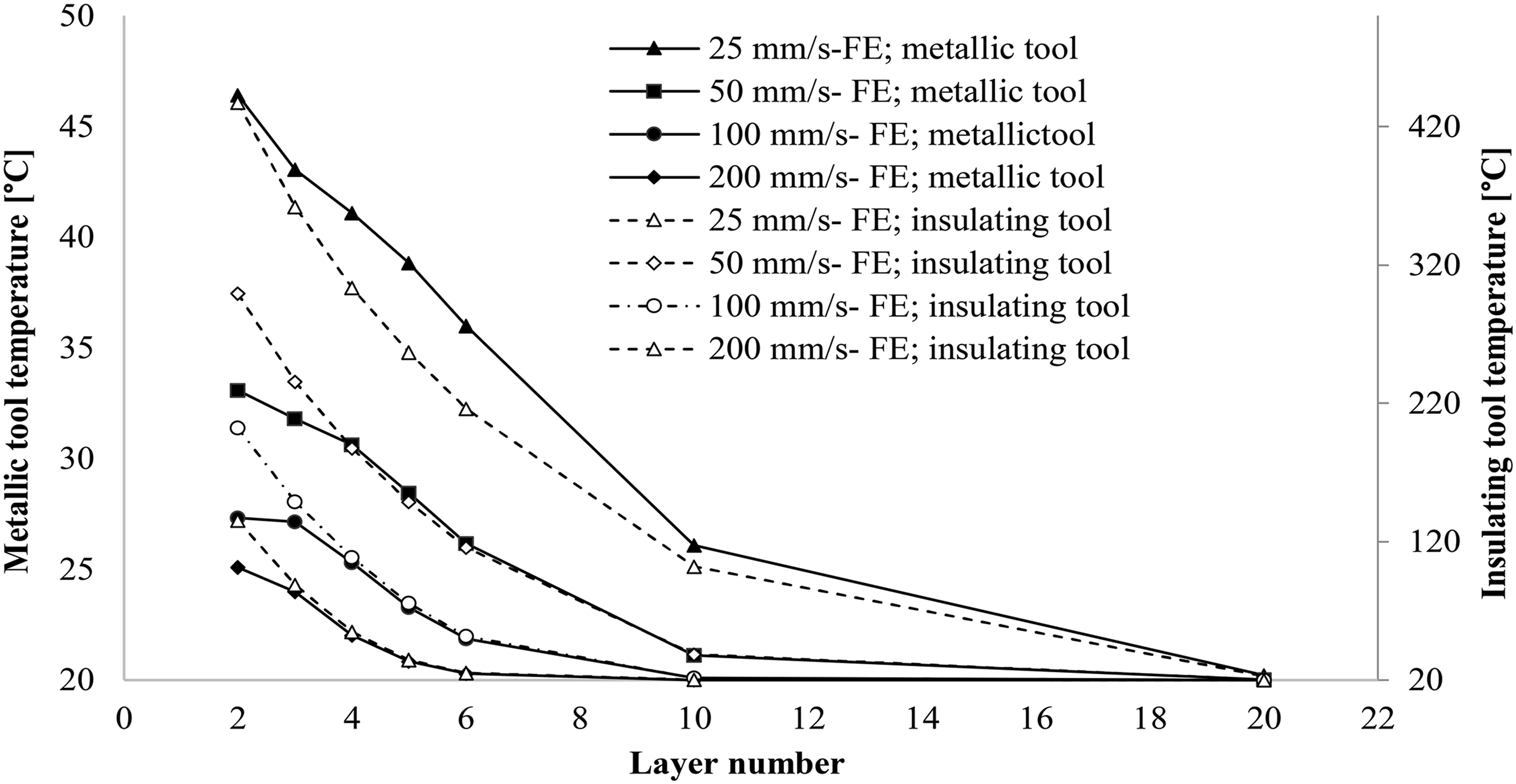
The approximation is in good agreement with the FE results as shown in Figure 7. A linear relation exists between the two sets of predictions which can be approximated by the identity line shown, with a coefficient of determination (R2) of 0.94. Approximately 85% of the scenarios present an error lower than 30°C whilst 45% of the total data present deviations of less than 10°C. The maximum deviation across all cases is 50°C, encountered in only 4 cases at the lowest speed of 25 mm/s for both tool materials. The deviations at 25 mm/s are high, ranging from 30–50°C, with the analytical scheme mostly overestimating the temperature. This is attributed to the constant thermal properties in the analytical calculations in contrast to the temperature dependence in the FE model. The average conductivity used in the approximation is 0.6 W/m/K for all scenarios, which is applied at a temperature of 180°C (Table 1) in the FE model. The temperatures achieved at 25 and 200 mm/s are up to 400 and 120°C respectively, which correspond to conductivities of 0.65 and 0.52 W/m/K in the FE model. As a result, the analytical predictions correlate well at temperature levels around the value of the average thermal properties and deviate at temperatures away from the average point used. Predictions at 25 mm/s are overestimates whilst predictions at 200 mm/s are underestimates, due to the lower and higher conductivity values used respectively. This can be seen also in Figure 7 where the predictions are in very good agreement below 200°C but gradually start deviating at higher temperatures. The second layer predictions have the highest error. This is attributed to the greater effect of energy losses to the tool during the first depositions, with the analytical formulation using a simplified approximation of these. As more layers are added, the influence of the tool is weaker and the heat loss to the tool becomes less important for the nip point prediction. For instance, the second ply deposition for the metallic tool at 50 mm/s presents an error of 34°C whereas for the third layer the error drops to 2°C.
Despite the simplification of the ATP geometry and heat transfer phenomena, the analytical scheme presents good predictive capability for a wide range of process conditions. It can describe the process and follow the nip point temperature evolution regardless of tool material. This is due to the use of a monitoring input in the form of tool temperature
Sensitivity of nip point temperature estimation to input parameters
The sensitivity of nip point estimations to the model parameter inputs is presented in Figure 9. The effect of a 10% increase in each variable individually is examined for the baseline scenario of a metallic tool at 50 mm/s process speed. For Sensitivity of the analytical scheme inputs to the predicted nip point temperatures for 10%, or 10°C, increase at different layers. Positive sensitivity denotes increase of the nip point value.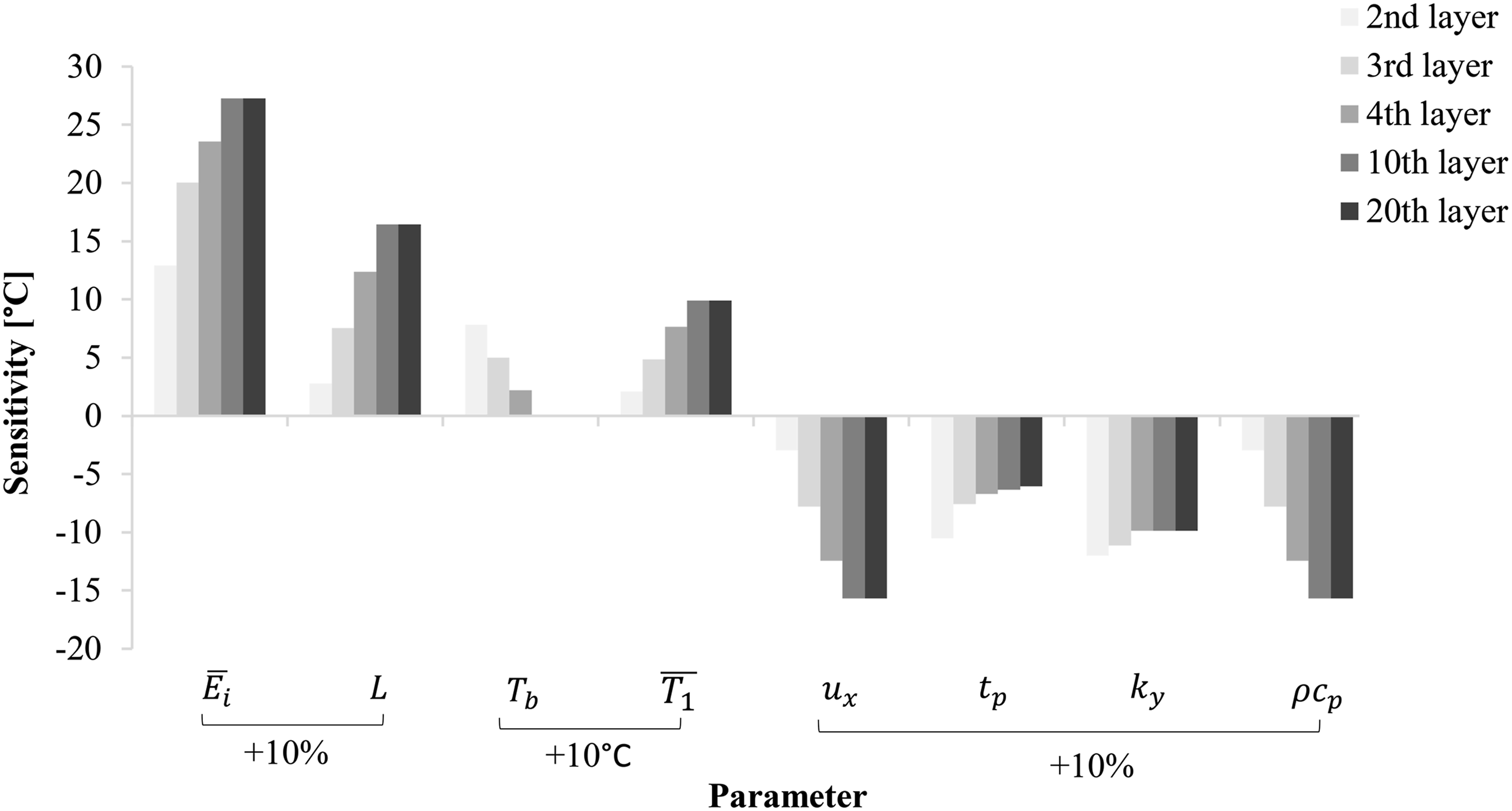
Example application to deposition under varying heater power
The in-process strategy proposed is demonstrated here in a virtual experiment simulated using the FE model. In this scenario, the deposition takes place on an insulating tool, with the properties reported in Table 1, at a speed of 50 mm/s. The tool features four temperature sensors placed 50 mm apart. The irradiance distribution on the tapes is constant across this straight placement path and equivalent to that of Figure 5, with a total irradiance value of 2.58 × 10⁵ W/m2. During the manufacture, the heater power is reduced to 75% of the initial value, linearly over the span of 1 s as shown in Figure 10(a). Three scenarios are examined that may take place during ATP manufacture: (i) the analytical nip point approximation is carried out knowing a priori the irradiance drop as part of process design; (ii) the power drop is unexpected and needs to be identified by the analytical scheme; (iii) no sensors are used in this tooling region progressing with predictions obtained away from this power variation. Processing at 50 mm/s with heater power drop: (a) FE profiles and analytical predicitions based on the available information for 2nd ply deposition; (b) errors of nip point temperatures inside the reduced power region for different number of layers.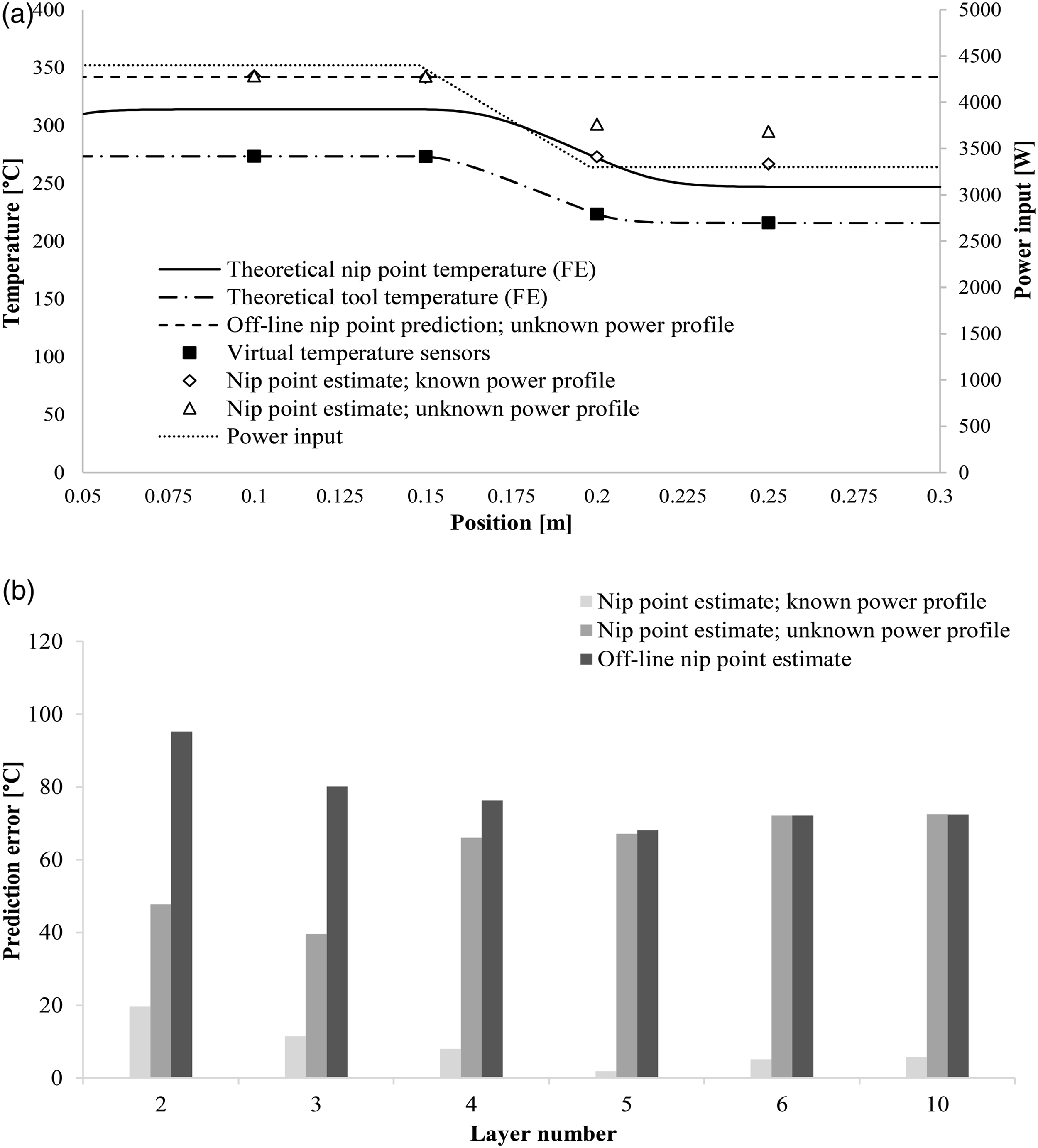
The nip point and tool profiles across the deposited length are plotted in Figure 10(a) for the second layer deposition alongside readings of the virtual sensors. When the power variation is known beforehand, the analytical prediction follows the nip point profile across the processed length satisfactorily, even in the transient region of decreasing power. In the case in which the power variation is not expected, the analytical predictions continue to follow the FE profile closely but with slightly greater error, up to 45°C. The estimation scheme acts in a monitoring sense, identifying the condition changes and potentially allowing their correction in future steps. In the case of solely off-line estimation, the change of nip point temperature is not measured, and predictions are almost 100°C off the theoretical.
The ability of the scheme to follow changes in conditions is also assessed in Figure 10(b) for different number of deposited layers. The analytical predictions inside the reduced-power region are within a 20°C error when the power variations are known. The potential to describe the resulting profile without this knowledge (case of unknown power variation) is good for the first four layers in which the estimation errors are lower than those of off-line studies. However, this capability is lost for thicker substrates due to the low sensitivity of tool temperature, as the heat transfer is shifted to conduction in a semi-infinite solid. The highest errors are obtained in the absence of process monitoring with an error of about 70–100°C.
This example highlights the role monitoring can play in ATP. The scheme allows identification of variations and translates them to changes in nip point temperature. The loss of monitoring capability as the thickness of the component is built up can be partially compensated for by information about the actual power profile obtained during the deposition of the first few layers, using the inverse calculation, which can then be used in a predictive way when the estimation operates in the semi-infinite solid regime.
Conclusions
An analytical approximation consisting of two 1D solutions was developed for estimating the nip point temperatures in ATP based on tool temperature measurements. The solutions address the two heat transfer regimes present in additive processes: heat conduction across a material interface while the deposited material has not reached large thicknesses and heat conduction in a semi-infinite solid governing the behaviour once substantial thickness of material has been built. The scheme is capable of utilising real-time temperature sensor data to estimate the power input profile of the heating source using an inverse solution that has a regularisation behaviour in the presence of significant noise in the temperature signals achieved through function specification of the profile. The nip point predictions assessed against data from a previously validated FE model show good correlation with an average error of 15°C, with the simplification of constant thermal properties and tool losses having the highest impact.
This work puts forward an approach for the heat transfer analysis of ATP which uses process data and simplified models instead of a comprehensive description of the problem requiring numerous high-uncertainty inputs and operating under ideal conditions. The simplicity and computational efficiency of predictions are well suited to in-process control algorithms. The potential to access approximate values of nip point temperature during the process generates the opportunity to control its value directly, therefore tuning the process to follow temperature profiles optimal in terms of layer bonding and material degradation. Industrial implementation of this approach is expected to trigger further developments, including simplified material transformation models and integration of sensors to supply the scheme with more accurate instantaneous conditions and information about material state. The power input has been addressed here through the inverse solution, but improvements on other critical parameters such as the material thermal properties and stack thickness are necessary, potentially including the effects of partial consolidation and inter-layer thermal resistance on the local effective conductivity.
Footnotes
Acknowledgements
Declaration of conflicting interests
The author(s) declared no potential conflicts of interest with respect to the research, authorship, and/or publication of this article.
Funding
The author(s) disclosed receipt of the following financial support for the research, authorship, and/or publication of this article: This work was supported by the Engineering and Physical Sciences Research Council through the EPSRC Centre for Doctoral Training in Composites Manufacture [grant number EP/L015102/1].