Modeling of induction heating of thermoplastic composites

Abstract

In this article, a hybrid finite element model is presented for the simulation of induction heating of layered composite plates. Modeling includes the alternating electromagnetic field generated by an alternating current running through a coil, the current densities in the composite plate resulting from the electromagnetic field, the heat generation resulting from the current density distribution, and the heat transfer resulting from the nonuniform heat generation in the plate and the temperature distribution in the plate. The different elements of the model are shown to capture the time-dependent temperature distribution resulting from a coil moving over the surface of a composite laminate.

Introduction

Thermoplastic components offer fusion bonding, also referred to as welding (see Figure 1 for a schematic representation), as an effective joining technology. Instead of bonding with a dedicated adhesive material, the matrix material in the composite plies themselves is used to form the bond in a welded joint. The polymer is locally heated until it liquefies, and pressure is applied so that an interface layer of liquid polymer emerges between the two welding components. After solidification, both components are joined together, forming a cohesive bond. ¹

Figure 1.

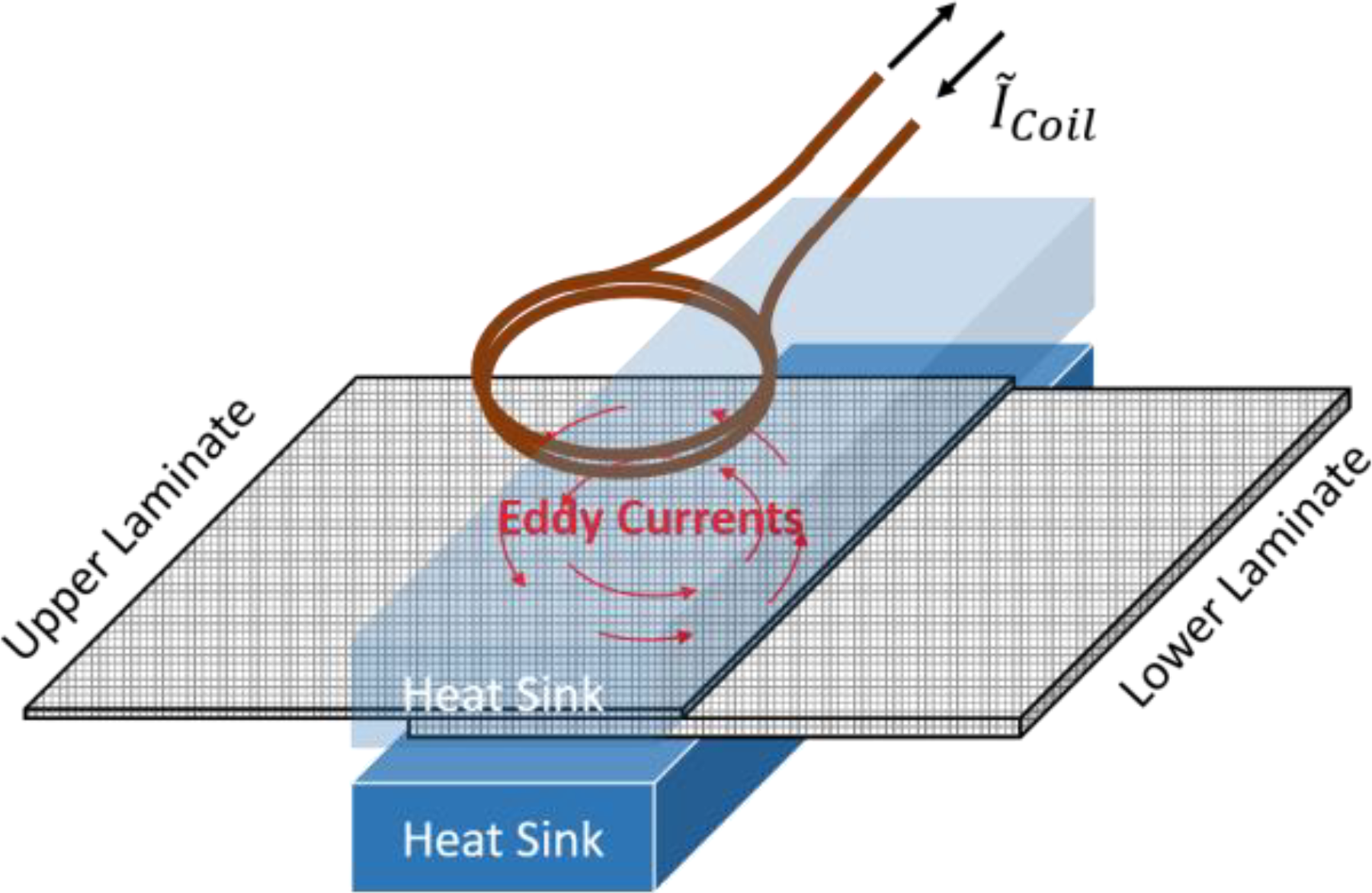
Basic elements required to perform induction welding of composites.

In the case of induction welding, eddy currents are used to generate the required heat to melt the thermoplastic polymer. These currents are induced in the electrically conductive carbon fiber reinforced polymer (CFRP) by a time-varying magnetic field. Electrical losses of the eddy currents result in heating of the material.^2,3 Induction heating allows for very rapid heating, locally concentrated where actually needed. ⁴ Since the induced currents act as a volumetric heat source, the process does not rely on heat conduction to transport the heat from the boundaries to the inside of the material and to the weld zone. This means that the heat source does not need to be placed on the composite, and the heat is not transferred from the contact point to the weld zone. Therefore, concentrated and fast heating is possible. By adding heat sinks at weld zone bottom and top, the temperature can be controlled and melting can be limited to the plate volume at the joint surface.

This approach varies from the more ‘traditional’ forms of welding of thermoplastics, (i) contact resistance, parts are welded by generating contact resistance (friction) at the interface of the component (common in plastics); (ii) electrical resistance, a resistive susceptor is placed at the interface between the components and heat is generated using a current, this however introduces a foreign material at the interface which is undesirable; and (iii) ultrasonic welding, high-frequency ultrasonic acoustic vibrations are used to weld components together.

If the electromagnetic force can induce current in the material, heating can occur due to (combinations of) (a) Joule heating of fibers, Figure 2(a) (b) Joule and/or dielectric heating of polymer, Figure 2(b) and (c) fiber-to-fiber contact resistance heating, ⁵ Figure 2(c). In all cases, effective heating requires a proper combination of induced currents and resistance since it is the volume integral of ${\vec{j}}^T{\sigma }^{-1}\vec{j}$ , with $\vec{j}$ being the current density and $\sigma$ being the 3-D conductivity tensor, which determines the total heat generated. The computational approach presented in this article is modeling the composite material as a continuum characterized by an anisotropic conductivity matrix. This matrix is rotated for each ply to match the ply’s fiber direction(s). The values of the entries in this matrix are based on measurements. This means that, except for dielectric heating of the polymer, all heating mechanisms are automatically included. Dielectric heating has not been included considering the low frequencies used for induction welding. The current density field resulting from the calculations can be used in combination with the conductivity matrices to investigate the dominant heating mechanism(s). Conductivity measurements done by the authors show the influence of fiber volume fraction and fiber distribution on the conductivity matrix.

Figure 2.

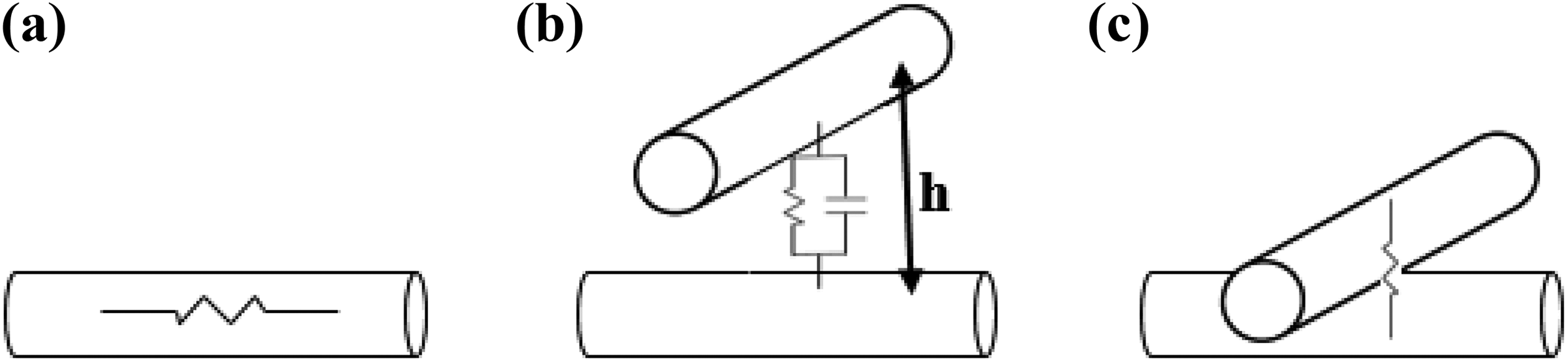
Induction heating mechanisms (a) Joule-based fiber heating, (b) Joule and/or dielectric polymer heating, and (c) contact resistance heating.

Modeling of induction welding of thermoplastic composites is a multi-scale, multi-physics problem and requires several different models to simulate all relevant aspects of the process. In the mesoscale simulation chain, at least an electromagnetic model and a heat transfer model are required to obtain the thermal response. Additional models can be utilized to further assess the thermal response, such as thermal stresses, deformations, and residual stresses.

The methodology discussed in the article does not require a presence of any resistive mesh susceptor. ²

Physical foundations and simulations strategy

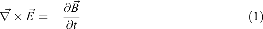
The fundamental mechanism of induction welding is heat generation in the substrate from induced electric currents. The induction of currents is a consequence of Faraday’s law, which implies that an alternating magnetic field $\vec{B}$ generates an electric field $\vec{E}$ ⁶

$\overrightarrow{\text{∇}}\times \vec{E}=-\frac{\partial \vec{B}}{\partial t}$

1

Both $\vec{B}$ and $\vec{E}$ are vector fields. $\overrightarrow{\text{∇}}\times \vec{E}$ denotes the curl of the electric field $\vec{E}$ . If an electrically conductive material is exposed to an electric field, electric currents are induced according to Ohm’s law ⁵

$\vec{j}=\sigma \vec{E}$

2

where $\vec{j}$ denotes the electric current density and $\sigma$ is the 3-D electrical conductivity tensor. The volumetric heat generation rate $\dot{Q}‴\left[\frac{W}{m^3}\right]$ can be calculated with Joule’s law

$\dot{Q}‴=\frac{{\partial }^{2}Q}{\partial V\partial t}=\vec{j}\cdot \vec{E}=\sigma \vec{E}\cdot \vec{E}$

3

Based on the volumetric heat generation rate, the temperature distribution $T\left(\vec{x},t\right)$ is obtained by solving Fourier’s equation for heat conduction in solids

$\rho c\frac{\partial T}{\partial t}=-\overrightarrow{\text{∇}}\cdot \left(\widehat{K }\overrightarrow{\text{∇}}T\right)+\dot{Q}‴$

4

Obtaining the temperature field is the most important objective of simulating induction heating. In a subsequent step, the temperature can be assessed in different respects considered essential for a successful weld.

Maxwell’s equations in context

The eddy current problem is governed by Maxwell’s equations, which have to be solved for a theoretically infinite domain including the coil, conductor (i.e. the laminate), and the surrounding space. Suggested among others by Rodriguez, ⁷ the four Maxwell equations can be written as follows

$\text{Maxwell-Ampere’ s law:} \frac{\partial \vec{D}}{\partial t}-\overrightarrow{\text{∇}}\times \vec{H}=-\vec{j}$

5

$\text{\hspace{0.5em}\hspace{1em}\hspace{1em}\hspace{1em}Faraday’s law:\hspace{0.5em}\hspace{1em}}\frac{\partial \vec{B}}{\partial t}+\overrightarrow{\text{∇}}\times \vec{E}=0$

6

$\text{Gauss’ magnetic law}:\hspace{1em}\overrightarrow{\text{∇}}\cdot \vec{B}=0$

7

$\text{Gauss’ electric law:\hspace{1em}\hspace{0.17em}}\overrightarrow{\text{∇}}\cdot \vec{D}={\rho }_c$

8

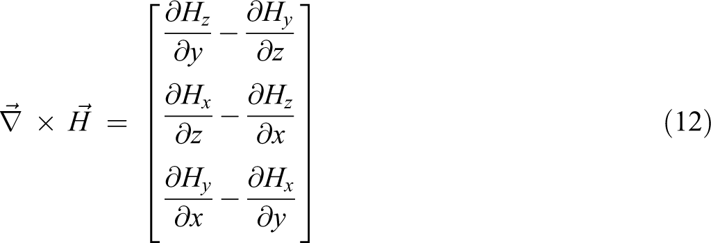
The magnetic field strength $\vec{H}$ and the magnetic induction $\vec{B}=\mu \vec{H}$ represent the magnetic field, where $\mu$ is the magnetic permeability. The current density $\vec{j}$ and the electric field $\vec{E}$ are related by the extended form of Ohm’s law

$\vec{j}={\vec{j}}^g+\sigma \vec{E}$

9

The use of tensor notation for $\sigma$ will enable the representation of anisotropic media such as fiber composites. The electric displacement field $\vec{D}$ is a measure for polarization of a dielectric material which is exposed to an electric field. It is related to the electric field by the permittivity $\epsilon$

$\vec{D}=\epsilon \vec{E}$

10

Finally, ${\rho }_c$ is the electric charge density. Maxwell’s equations make use of the differential vector operators divergence and curl

$\overrightarrow{\text{∇}}\cdot \vec{B}=\frac{\partial B_x}{\partial x}+\frac{\partial B_y}{\partial y}+\frac{\partial B_z}{\partial z}$

11

$\overrightarrow{\text{∇}}\times \vec{H}=\left[\begin{array}{l}\frac{\partial H_z}{\partial y}-\frac{\partial H_y}{\partial z}\hfill \\ \frac{\partial H_x}{\partial z}-\frac{\partial H_z}{\partial x}\hfill \\ \frac{\partial H_y}{\partial x}-\frac{\partial H_x}{\partial y}\hfill \end{array}\right]$

12

For the eddy current problem, two major simplifications are frequently applied. The first one is the low-frequency approximation which neglects the time derivative of electric displacements, that is, $\frac{\partial \vec{D}}{\partial t}\approx 0$ . This basically means that capacitive effects due to the rapidly changing electric field are ignored in the eddy current model. ⁸ While there is no general error estimate, Bossavit ⁸ suggests that this approximation may be valid for excitation frequencies up to as high as 10 MHz and even above, depending on the application. For the induction welding process, excitation frequencies in the range of 200–300 kHz are applied. Since this approximation is used in most publications and local inaccuracies are not considered a particular problem, the approximation is accepted for induction welding without further justification.

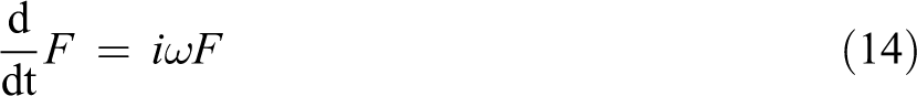
Next to neglecting capacitive effects, the second simplification is to introduce the time harmonic notation for all alternating field quantities (p. 63). ⁷ It applies to all quantities which vary periodically in time and follow a sinusoidal function. This is the case if the source current of the exciting coil is an alternating current, which is true for induction welding. Under these circumstances, all other time-dependent field quantities are also sinusoidal functions and can be represented as the real part of a complex valued harmonic function

$F\left(\vec{x},t\right)=\text{\hspace{0.17em}Re}\left[F_c\left(\vec{x}\right)e^{i\omega t}\right]$

13

where $F_{\text{c}}$ is the complex-valued amplitude and $\omega =2\pi f$ is the angular frequency of the exciting current. In consequence, the time derivatives of these harmonic functions can be written in the form

$\frac{\text{d}}{\text{dt}}F=i\omega F$

14

Both simplifications yield the low-frequency, time-harmonic Maxwell equations ⁷

$\overrightarrow{\text{∇}}\times \vec{H}=\vec{j}$

15

$i\omega \mu \vec{H}+\overrightarrow{\text{∇}}\times \vec{E}=0$

16

$\overrightarrow{\text{∇}}\cdot \left(\mu \vec{H}\right)=0$

17

$\overrightarrow{\text{∇}}\cdot \left(\epsilon \vec{E}\right)=\rho$

18

$\vec{j}={\vec{j}}^g+\sigma \vec{E}$

19

As a side note, equation (19), Ohm’s law, is not part of the Maxwell equations in the strict sense. This set of equations forms the basis for the derived finite element formulation.

Weak form

To solve the eddy current problem in general, one has to consider not only the conductive domain $C$ but also the infinite outside region $O$ . Both are separated by a boundary surface $S$ . Figure 3 indicates these regions. By applying a source current to the induction coil, a magnetic field is generated. This field reaches out to infinite space and can be calculated with the Biot–Savart law. However, eddy currents induced in $C$ in return change the magnetic field in the entire domain.

Figure 3.

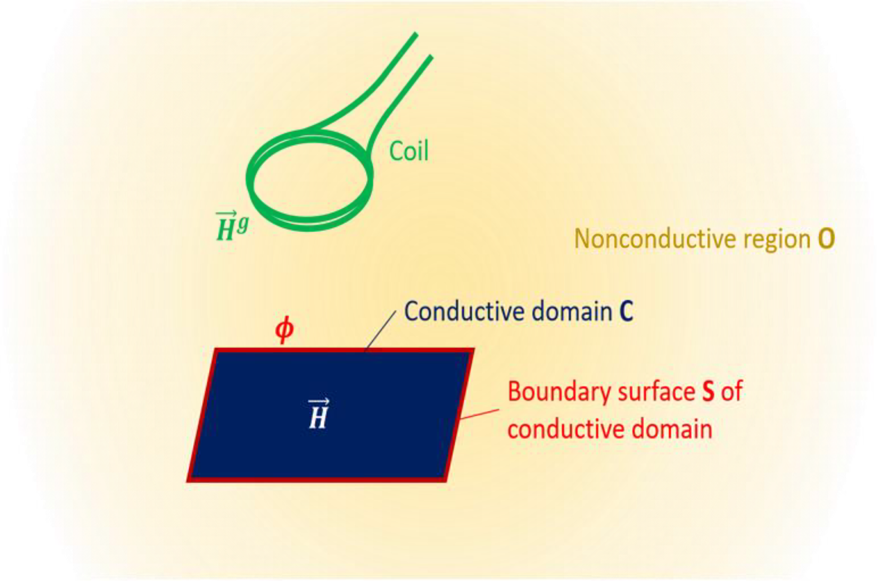
Regions of the eddy current problem.

Because of this interdependence, the effective magnetic field and the resulting eddy currents can only be calculated by solving the Maxwell equations for the entire problem. For that reason, common commercial finite element method (FEM) software solutions, for example, ANSYS Maxwell or COMSOL, ⁹ require explicit modeling and discretization of not only the conductor but also the coil as well as the surrounding air. As opposed to those commercial solutions, the implemented method only requires discretization of the conductive domain, which considerably reduces the number of elements needed. On the other hand, the influence of components outside of the analyzed conductive domain cannot be directly accounted for.

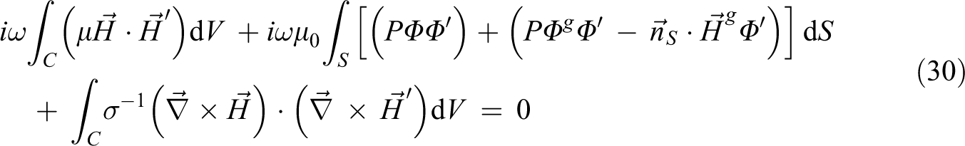
The following derivation reproduces the steps taken by Bossavit, ⁸ without the mathematical proofs. To obtain a weak formulation, equation (16) is multiplied by a test function $\vec{H}\prime$

${\displaystyle {\int }_{\text{Ω}}\left(i\omega \mu \vec{H}+\overrightarrow{\text{∇}}\times \vec{E}\right)\cdot \vec{H}\prime \text{\hspace{0.17em}d}V}=0$

20

Applying the curl integration by parts formula

$i\omega {\displaystyle {\int }_{\text{Ω}}\left(\mu \vec{H}\cdot \vec{H}\prime \right)\text{d}V}+{\displaystyle {\int }_{\text{Ω}}\left(\vec{E}\cdot \left(\overrightarrow{\text{∇}}\times \vec{H}\prime \right)\right)\text{d}V}=0$

21

It is now necessary to treat different parts of the infinite electromagnetic domain separately. The total domain $\Omega$ consists of a conductive domain $C$ and a nonconductive domain $O$ (mainly air). They share a common boundary $S$ (see Figure 2). In the nonconductive domain, there can be no electric current

$\vec{j}=\overrightarrow{\text{∇}}\times \vec{H}\prime =0\text{\hspace{0.17em}in\hspace{0.17em}}O$

22

The source current ${\vec{j}}^g$ is zero in $C$ by definition, and thus, the electric field can be substituted with Ohm’s law, equation (19), and Ampere’s law, equation (15)

$\vec{E}={\sigma }^{-1}\vec{j}={\sigma }^{-1}\left(\overrightarrow{\text{∇}}\times \vec{H}\right)$

23

With these relations, equation (21) now becomes

$\begin{array}{l}i\omega {\displaystyle {\int }_{\text{Ω}}\left(\mu \vec{H}\cdot \vec{H}\prime \right)\text{d}V}+{\displaystyle {\int }_C{\sigma }^{-1}\left(\overrightarrow{\text{∇}}\times \vec{H}\right)\cdot \left(\overrightarrow{\text{∇}}\times \vec{H}\prime \right)\text{d}V}=0\\ \end{array}$

24

For what follows, $C$ is assumed to be contractible, which means in essence that there cannot be any holes or loops. Since there is no source current in $C$ , the source magnetic field can be written as the gradient of a scalar potential field

${\vec{H}}^g=\overrightarrow{\text{∇}}{\Phi }^g\text{\hspace{1em}in }C\text{\hspace{0.17em}including\hspace{0.17em}}S$

25

Furthermore, the response magnetic field is formulated in the nonconductive domain

$\vec{H}={\vec{H}}^g+\overrightarrow{\text{∇}}\left(\Phi -{\Phi }^g\right)\text{\hspace{0.17em}in\hspace{0.17em}}O$

26

$\vec{H}\prime ={\vec{H}}^g+\overrightarrow{\text{∇}}\left(\Phi \prime -{\Phi }^g\right)\text{\hspace{0.17em}in\hspace{0.17em}}O$

27

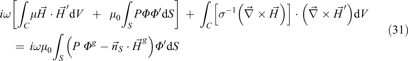
Thus, the first integral in equation (24) can be split

$i\omega {\displaystyle {\int }_{\text{Ω}}\mu \vec{H}\cdot \vec{H}\prime \text{d}V}=i\omega {\displaystyle {\int }_C\mu \vec{H}\cdot \vec{H}\prime \text{d}V}+i\omega \underset{O}{\int }\mu \left({\vec{H}}^g+\overrightarrow{\text{∇}}\left(\Phi -{\Phi }^g\right)\right)\cdot \left({\vec{H}}^g+\overrightarrow{\text{∇}}\left(\Phi \prime -{\Phi }^g\right)\right)\text{d}V$

28

Henceforth, there are two variables, $\vec{H}$ and $\Phi$ . Now the “Dirichlet-to-Neumann” map is introduced, see the work of Bossavit ⁸ (pp. 205 ff.)

$P:{\Phi }_S\to \frac{\partial \Phi }{\partial n_S}$

29

P maps a Dirichlet condition ${\Phi }_S$ of the elliptical problem to an equivalent Neumann condition $\frac{\partial \Phi }{\partial n_S}$ on a surface S. Utilizing the properties of P, the integral over the nonconductive domain $O$ in equation (28) can be reduced to an integral over the boundary surface $S$ , resulting in the final weak formulation (p. 229) ⁷

$i\omega {\displaystyle {\int }_C\left(\mu \vec{H}\cdot \vec{H}\prime \right)\text{d}V}+i\omega {\mu }_0{\displaystyle {\int }_S\left[\left(P\Phi \Phi \prime \right)+\left(P{\Phi }^g\Phi \prime -{\vec{n}}_S\cdot {\vec{H}}^g\Phi \prime \right)\right]}\text{\hspace{0.17em}d}S+{\displaystyle {\int }_C{\sigma }^{-1}\left(\overrightarrow{\text{∇}}\times \vec{H}\right)\cdot \left(\overrightarrow{\text{∇}}\times \vec{H}\prime \right)\text{d}V}=0$

30

Finally, the load terms are switched to the right-hand side of the equation

$i\omega \left[{\displaystyle {\int }_C\mu \vec{H}\cdot \vec{H}\prime \text{d}V}+{\mu }_0{\displaystyle {\int }_{S}P\Phi \Phi \prime \text{d}S}\right]+{\displaystyle {\int }_C\left[{\sigma }^{-1}\left(\overrightarrow{\text{∇}}\times \vec{H}\right)\right]\cdot \left(\overrightarrow{\text{∇}}\times \vec{H}\prime \right)\text{d}V}=i\omega {\mu }_0{\displaystyle {\int }_S\left(P{\text{ Φ}}^g-{\vec{n}}_S\cdot {\vec{H}}^g\right)\Phi \prime \text{d}S}$

31

As opposed to other methods, there are two state variables in this formulation. $\vec{H}$ is the variable magnetic field inside the conductive domain $C$ . It is complemented by the scalar potential $\Phi$ on the boundary surface $S$ , where the relation $\vec{H}=\overrightarrow{\text{∇}}\Phi$ holds true. Suitable discrete representations of both variables are elaborated throughout the next section.

Finite element discretization

To discretize the weak formulation, both variables are expanded with suitable shape functions. The scalar variable $\Phi$ is discretized with nodal shape functions on the boundary surface $S$ . The vector quantity $\vec{H}$ can be reduced to a scalar degree of freedom with the use of the so-called edge elements. With this type of finite element, the degrees of freedom are assigned to the edges rather than the nodes (pp. 108 ff.). ¹⁰ Thus, the orientation of a vector quantity is defined by the orientation of an edge of the element and its magnitude is defined by a scalar degree of freedom on this edge. Edge elements are curl-conforming, that is, the curl of field quantities is square integrable.

To discretize the carbon fiber laminates to be joined by induction welding, hexahedral mixed elements are used. The term “mixed” originates from the ability of the element type to bear degrees of freedom on its edges for vector quantities, on its nodes for scalar quantities, and on its surfaces for areal quantities. This kind of element was first described and defined by Nedelec ¹¹ for the three-dimensional case. Based on the work of Nedelec, ¹¹ Miyata ¹² provides a detailed collection of isoparametric mixed elements including their nodal and edge shape functions. His hexahedral element (pp. 63–64), ¹² as shown in Figure 4, is used to discretize the induction welding problem. The hexahedral element has 8 nodes and 12 edges. By convention, indices i and j shall denote node indices, and p and q shall denote edge indices. Miyata ¹² defines the following shape functions for nodes and edges

Figure 4.

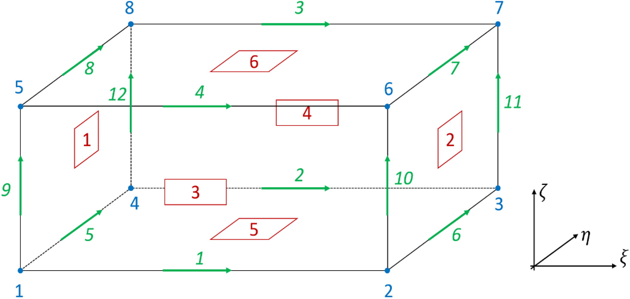
Isoparametric hexahedral mixed element. ¹²

$N_i=\frac{1}{8}\left(1+{\xi }_i\xi \right)\left(1+{\eta }_i\eta \right)\left(1+{\zeta }_i\zeta \right) \text{for nodes}$

32

${\vec{N}}_p=\frac{1}{8}\left(1+{\xi }_p\xi \right)\left({\eta }_p\eta \right)\left({\zeta }_p\zeta \right)G{\left[{\delta }_{\xi }^p{\delta }_{\eta }^p{\delta }_{\zeta }^p\right]}^T \text{for edges}$

33

Using the shape functions, the final discrete system describing the heating problem becomes (p. 229) ⁹

$i\omega \left(M\left(\mu \right)+{\mu }_{0}P\right)\kappa +N\left(\sigma \right)\kappa =i\omega {\mu }_0\left(P{\Phi }^g-L^g\right)$

34

The matrix $M$ is based on the first integral of equation (31), while the matrix $N$ is based on the third integral in the weak form, equation (31). An approximate discretization of the integrals involving the Dirichlet-to-Neumann map P is given by Bossavit. ⁸ The resulting matrix is called the “discrete Dirichlet-to-Neumann map” $P$ .

Notably, the magnetic field $\vec{H}$ is expressed through edge degrees of freedom inside the conductive domain C and through $\overrightarrow{\text{∇}}\Phi$ on the boundary surface S. Its discrete expansion is thus

$\vec{H}=\sum _p^{ }{H}_p{\vec{N}}_p+\sum _i^{ }{\Phi }_i\overrightarrow{\text{∇}}{\text{N}}_i$

35

Loads and boundary conditions

Naturally, the second part involving nodal degrees of freedom only applies to boundary elements of C. All degrees of freedom on the edges, H_p, and nodes, ${\Phi }_i$ , are combined in a single vector of degrees of freedom, $\kappa$ . Considering the test functions for edges, ${\vec{H}\prime }_q={\vec{N}}_q$ , and surface nodes, ${\vec{H}\prime }_j=\overrightarrow{\text{∇}}{\text{N}}_j$ , the matrices N and M are composed of four sub-matrices: One relates edges to edges (p, q), another one relates nodes to nodes (i, j), and there are two sub-matrices coupling edge and nodal degrees of freedom, (p, j) and (i, q). Whereas N is nonzero only in the edge–edge part, M is fully occupied and thus accounts for coupling between edges and nodes.

For the current finite element formulation, it is necessary to compute the source magnetic field ${\vec{H}}^g$ generated by the electromagnetic coil. The source magnetic field ${\vec{H}}^g$ and the source magnetic scalar potential ${\Phi }^g$ are computed with the Biot–Savart law. It gives a general solution for a 1-D wire loop in 3-D space ⁶

${\vec{H}}^g\left(\vec{x}\right)=\frac{1}{4\pi }\int \frac{I{\vec{e}}_{12}\times d{\vec{s}}_2}{r_{12}^2}$

35

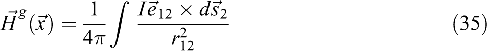
By evaluating the Biot–Savart law for all boundary surface nodes of the mesh, the discrete magnetic field $H^g\left(x,y,z\right)$ is obtained. The scalar magnetic potential ${\Phi }^g$ on the boundary surface is defined as

$\overrightarrow{\text{∇}}{\Phi }^g=H^g$

36

The difference in the potential between two points can be calculated as the line integral of the gradient field along any arbitrary path between these two points ⁶ (pp. 3–4)

${\Phi }_2-{\Phi }_1={\displaystyle {\int }_1^2\overrightarrow{\text{∇}}\Phi \cdot \overrightarrow{\text{d}s}}={\displaystyle {\int }_1^2\vec{H}\cdot \overrightarrow{\text{d}s}}$

37

In practice that means that ${\Phi }^g$ can be set to zero at any node of the mesh. Starting from this node, ${\vec{H}}^g$ is integrated along all edges of the mesh to retrieve the scalar potential ${\Phi }^g$ on all nodes of the boundary surface. The load vectors ${\Phi }^g$ and $L^g$ in equation (34), are nonzero only for the surface node degrees of freedom. There are no direct loads on the internal edge degrees of freedom H_p, but they are coupled to the surface loads by the $M$ matrix. If there are several load steps, only ${\Phi }^g$ and $L^g$ have to be recalculated, whereas $M$ , $N$ , and $P$ stay the same. This makes the code efficient in calculating problems with a movable coil. Thereby each load case is a quasi-static problem and can be solved individually.

Next to the load calculations, modeling the induction welding process of a CFRP laminate at this point only requires one boundary condition: There must be no currents across the boundary surface of the conductive domain. This condition is satisfied by default by the implemented code. This is because the magnetic field $\vec{H}$ on the boundary surface $S$ and in the nonconductive domain $O$ is given as the gradient of the scalar magnetic potential, as introduced in the fourth section

$\vec{H}=\overrightarrow{\text{∇}}\Phi$

38

Hence, all currents in the nonconductive domain including the boundary surface are

$\vec{j}=\left(\overrightarrow{\text{∇}}\times \vec{H}\right)=\left(\overrightarrow{\text{∇}}\times \left(\overrightarrow{\text{∇}}\Phi \right)\right)=0$

39

since gradient fields are always curl-free. Thus, there can be no currents across the boundary surface.

Finally, modeling of multilayered structures requires coupling conditions between the different layers. This is achieved by merging coincident nodes on the common boundaries. This amounts to perfect electrical coupling between the layers. In case experimental validation results demand the modeling of imperfect coupling, another solution will have to be implemented for this condition.

By solving the linear equation system equation (34), the response magnetic field is obtained for the conductive domain $C$ . One obtains the magnetic field inside an element from its edge and node degrees of freedom

$\vec{H}\left(x,y,z\right)=\sum _{p\in {\mathbb{E}}_C}{H}_p{\vec{N}}_p+\sum _{i\in {\mathbb{N}}_S}{\Phi }_i\overrightarrow{\text{∇}}{N}_i$

40

The second term is only relevant for elements that have at least one boundary surface element.

For the quantification of induction heating, the electric current density $\vec{j}$ is required, which can be calculated with Ampere’s law

$\vec{j}=\overrightarrow{\text{∇}}\times \vec{H}$

41

$=\overrightarrow{\text{∇}}\times \left(\sum _{p\in {\mathbb{E}}_C}{H}_p{\vec{N}}_p+\sum _{i\in {\mathbb{N}}_S}{\Phi }_i\overrightarrow{\text{∇}}{N}_i\right)$

42

$=\sum _{p\in {\mathbb{E}}_C}{H}_p\left(\overrightarrow{\text{∇}}\times {\vec{N}}_p\right)+\sum _{i\in {\mathbb{N}}_S}{\Phi }_i\left(\overrightarrow{\text{∇}}\times \overrightarrow{\text{∇}}{N}_i\right)$

43

The discrete curl, as defined by Miyata (p. 64), ¹² can be used to directly compute $\vec{j}$ from the edge values H_p. Finally, the power dissipated by the eddy currents can be calculated. It is essential that the calculated quantity $\vec{j}$ is not the actual current density, but the phasor of a harmonic function, as defined in equation (13). Henceforth, this current density phasor will be denoted by $\underset{\_}{\widehat{j}}$ to distinguish it from the actual current density $\vec{j}$

$\vec{j}\left(t\right)=\text{Re}\left[\underset{\_}{\widehat{j}}{e}^{i\omega t}\right]$

44

The real amplitude of the signal is denoted by $\widehat{j}$ , which is still a vector with three components. The time-averaged dissipated power can be calculated from the effective current density of a sinusoidal alternating current

${\vec{j}}_{\text{eff}}=\frac{\widehat{j}}{\sqrt{2}}$

45

Finally, the average dissipated power is calculated

$\widehat{\dot{Q}}‴={\sigma }^{-1}{\vec{j}}_{\text{eff}}\cdot {\vec{j}}_{\text{eff}}=\frac{1}{2}{\sigma }^{-1}\widehat{j}\cdot \widehat{j}$

46

A prerequisite for this result is that capacitances and inductances in the material are negligible so that there is no phase shift between current density and the electric field. The dissipated electrical power is assumed identical with the heating rate per unit volume, which is the desired result of the eddy current simulation.

Temperature field assessment

In the case of induction welding, with heat being generated inside of the welding work pieces, the governing mode is heat conduction through the components. Convection and radiation may appear as boundary conditions, helping to cool down the material on its surface. The energy conservation equation for heat conduction in a solid with constant material properties is Fourier’s equation of heat conduction (p. 277) ¹³

$\rho c\frac{\partial T}{\partial t}=-\overrightarrow{\text{∇}}\cdot \left(\widehat{K} \overrightarrow{\text{∇}}T\right)+\dot{Q}‴$

47

From the eddy current simulation and subsequent heat transfer simulation, the time-dependent temperature field $T\left(\vec{x},t\right)$ is obtained. The temperature field is vital to predict the quality of the welded joint. First and foremost, there is a restricted temperature range that allows for a successful fusion bond. Its lower end is the melting temperature of the thermoplastic matrix material. It has to be exceeded for a certain duration to make sure the thermoplastics are fully melted at the bonding interface. The upper limit of the corridor is marked by the beginning of thermal degradation of the thermoplastic matrix. Exceeding it leads to deteriorated mechanical properties.

The outlined methods are vital to identify and analyze problems in the welding process before they occur. Slight changes in the process parameters or even the joint design may enable significant gains in quality. Hence, temperature field assessment is a key aspect of analysis and optimization of the induction welding process.

Induction welding simulation example

The method described is implemented in a MATLAB code and is applied to model the induction welding process of two laminated CFRP components. In the presented example, each of the components is a flat plate with dimensions 250 × 150 mm². These plates are joined with induction welding in a lap joint configuration (see Figure 5). The ply orientations are $\left[0/90/90/0\right]$ for the upper laminate and $\left[90/0/0/90\right]$ for the lower one, with each ply having a thickness of 0.25 mm. Ceramic heat sinks are applied at the top and the bottom of the joint to avoid overheating of the laminates. They are both modeled as blocks and have a rectangular cross section with dimensions 100 × 12.5 mm².

$\sigma =\left[\begin{array}{ccc}9827.27& & \\ & 1.3& \\ & & 0.0816\end{array}\right]\mathrm{\hspace{1em}\hspace{1em}\hspace{1em}\hspace{1em}\mu }=1.2566\times {10}^{-6}$

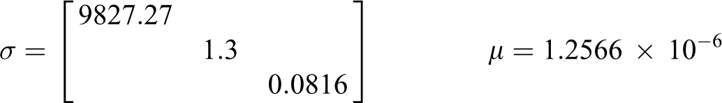
The coil is shaped as a single hairpin (represented by red in Figure 6) and placed vertically, that is, in the x–z plane, above the laminate. The frequency and current were set to 275 kHz and 575A, respectively. The coil moves along the joint at a constant feed rate (0.25 of the plate length per step). A set of material parameters were applied (the electrical conductivity $\sigma$ and magnetic permeability $\mu$ are given previously), representative for welding of, for example,polyphenylene sulfide (PPS) or polyetherketoneketone (PEKK) with carbon fibers. The simulation is a two-step approach, first the heat body flux in the elements are determined, and second, a heat transfer analysis is performed. For the heat body flux calculations, the heat sinks are not required to be present, this is displayed in Figure 5, which shows the induced heating power during a lap joint welding process.

Figure 5.

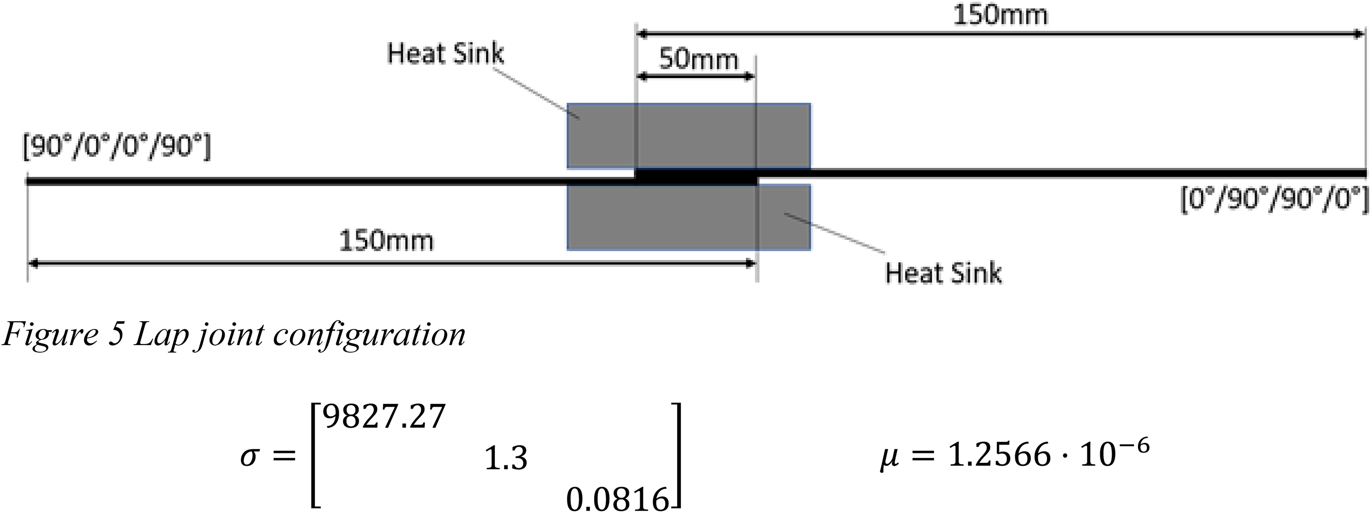
Lap joint configuration.

Figure 6.

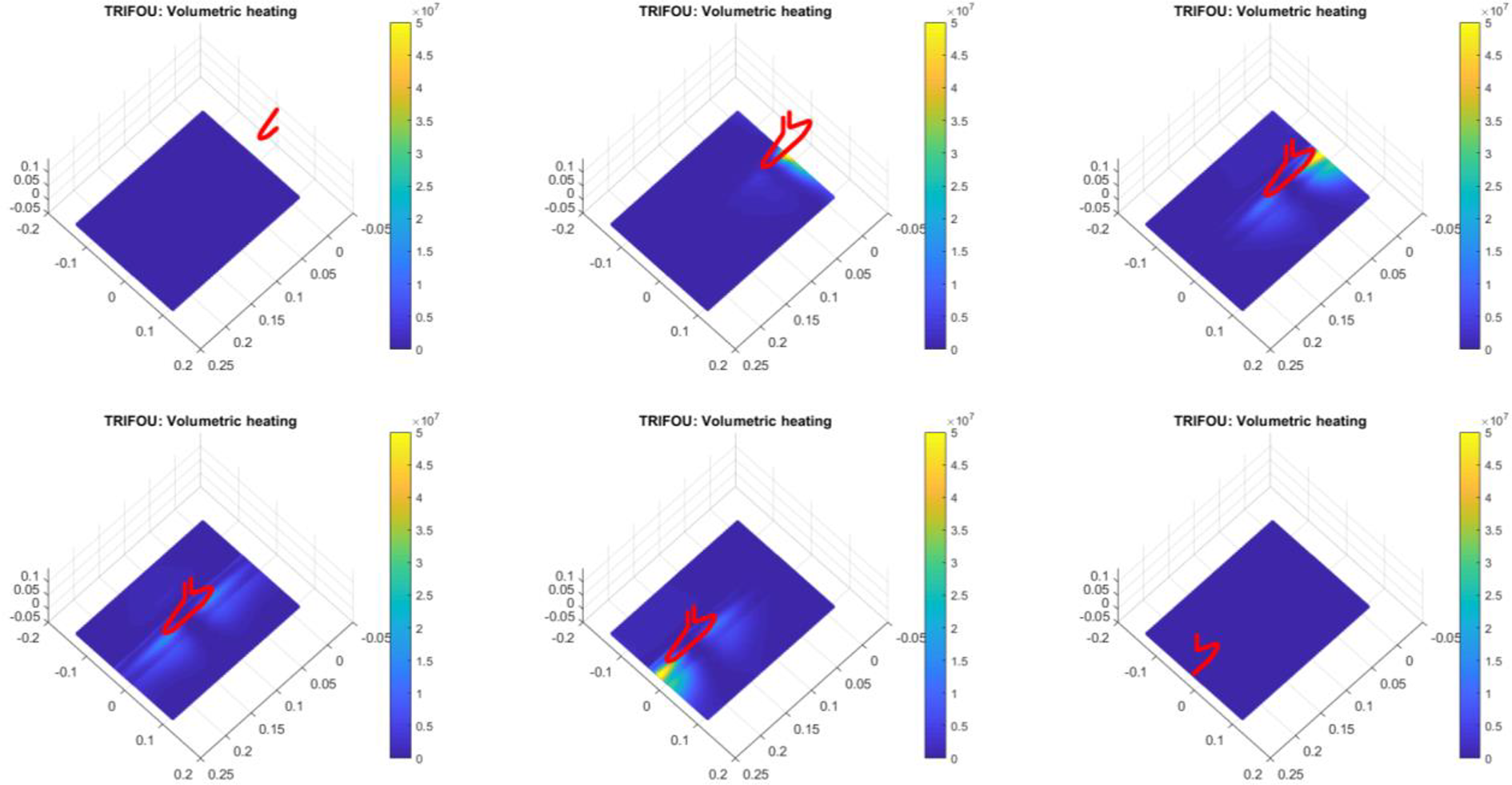
Induced volumetric heat generated during a lap joint welding process.

Next, using the eddy current analysis results (the induced heating power $\dot{Q}‴$ ) is used in the heat transfer analysis model. In this case, the coil was held for 2 s at each position, and the resulting temperature shown in Figure 7 corresponds to the coil positions 1, 3, and 4 shown in Figure 6.

Figure 7.

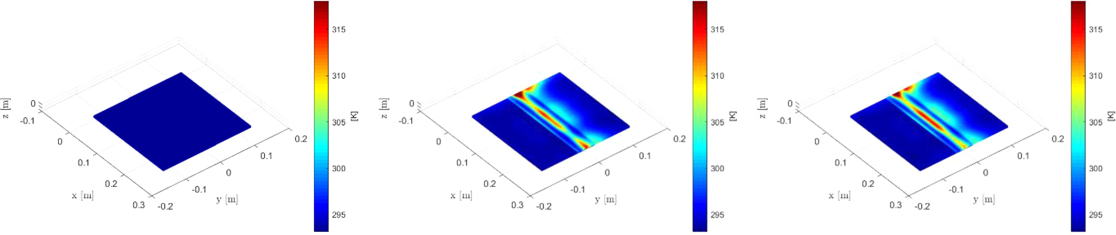
Temperature during the lap joint welding process without heat sinks.

Figure 7 shows that the maximum heating occurs in the area where the laminates overlap, which is desirable. However, Figure 7 also shows significant heat generated at the top surface of the overlap region. Heating at the top is unwanted as it does not contribute to cohesion bond, and it will produce an undesired surface finish quality. One can reduce this unwanted heating through active (e.g. cold air) cooling, or one can add heat sinks at the top and bottom to reduce the temperature at the surface (see Figure 8).

Figure 8.

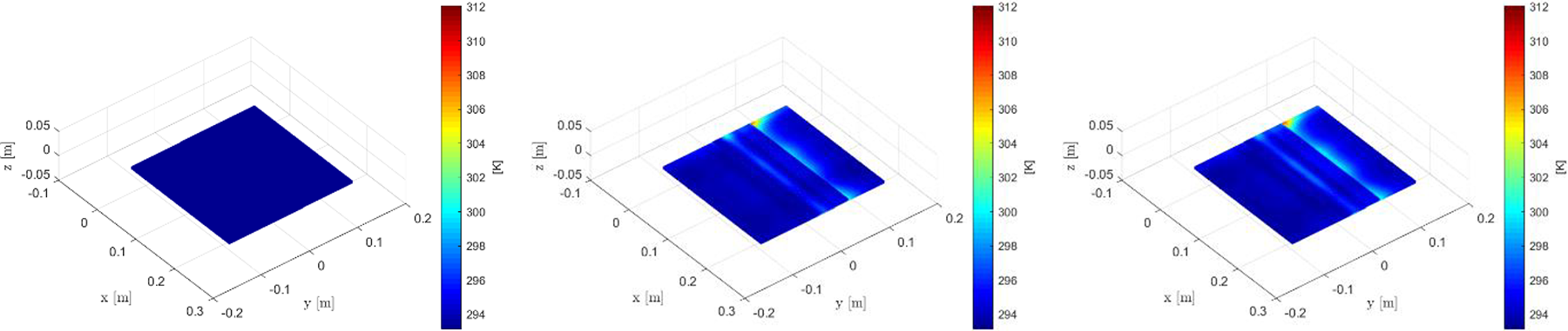
Temperature during the lap joint welding process with heat sinks.

To highlight the difference in surface temperate with and without heat sinks, the top heat sink is partially removed (for illustration purposes only); and the generated heat without heat sinks (Figure 7) and with heat sinks (Figure 8) are compared. As it can be seen from Figure 8, the temperature at the surface is reduced due to the presence of the heat sinks; therefore, one can use heat sinks to control the surface temperature and prevent any unwanted heating at the surface.

Furthermore, by modification of the welding parameters (such as coil speed, current, or frequency) the proper temperature at each location can be achieved.

In addition to the numerical simulations, a quantitative validation was performed. Two thermoplastic composite plates in a lap shear joint configuration were welded, of which the result is shown in Figure 10. As it can be seen from Figure 10, two heat spots are present at the edge at which the induction coil “enters” the plates. These two heat spots were captured by the numerical tool as can be seen from Figure 9.

Figure 9.

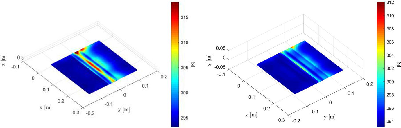
Temperature at the surface: (left) without heat sinks and (right) with heat sinks.

Figure 10.

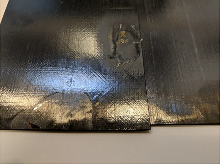
Experimental induction weld.

Conclusions and future work

The weak formulation and discretization of the Maxwell equations as given by Bossavit ⁸ is shown to be a useful formulation to capture the heating of composite layered plates in a magnetic field. The calculated volumetric heat generation was used as input for the body forces of a heat transfer problem. The combination of the two codes allowed the simulation of welding a lap joint between two composite plates. The simulation included an elliptical coil moving over the length of the lap joint. Heat sinks were applied to resemble a practical welding setup.