Microscopic level modeling of induction welding heating mechanisms in thermoplastic composites

Abstract

Simulation and analysis of electromagnetic induction heating of continuous conductive fiber-based composite materials is used to (in)validate a series of hypotheses on the physics dominating the heating process. The behavior of carbon fibers with and without surrounding polymer in an alternating electromagnetic field is studied at a microscopic level in ANSYS Maxwell using the solid loss to quantify heat generation in the composite material. To limit the number of elements, the fibers are modeled with a polyhedron cross-section instead of a circular cross-section. In addition, each layer is modeled as an layer of fibers, e.g. 20 fibers placed next to each other. The simulations indicate that samples with fibers oriented in 0 and 90 orientation yield a substantial higher solid loss than fibers oriented in the 0 orientation only. The solid loss in both cases is however not enough to explain the level of heating observed in practice. Filling the volumes between fibers with polymer results in greater solid loss than samples with no polymer between the fibers, at equal fiber volume fraction. Note, no contact between fibers is modeled. The conductivity of the polymer is experimentally determined. The lab tests show relatively low finite resistance values in the transverse direction, indicating that the polymer in a composite should not be considered an isolator. The simulations seem to justify the conclusion that heating of thermoplastic composites in an alternating magnetic field rely on currents through the polymer. Without the polymer and subsequently no polymer conductivity, even if the electrical fields are strong there is almost no heat generated. The carbon fibers are required to be in proximity of each other to create the electrical fields that induce the current through the polymer. The heating is determined by the product of current density squared times the resistivity of the polymer.

Introduction

Thermoplastic composites (TPCs) offer high damage tolerance compared to their thermoset counterparts. In addition, the thermoplastic resin system opens the possibility to fusion bond two thermoplastic components together without the need for an adhesive, or mechanical fasteners. ¹ Several fusion bonding methodologies exists, like ultrasonic welding, resistance welding and induction welding just to name a few. ² This manuscript focuses on induction welding only as it possesses advantages (such as, contactless, localized and rapid heating) with respect to other fusion bonding methodologies.

The induction welding process (schematically given in Figure 1) relies on the generation of eddy currents within the TPC. The eddy currents are the result from an alternating current (AC) passing through an inductive coil with a fixed or varying frequency. As the current flows back and forth through the coil, it produces an alternating electromagnetic (EM) field as described by Faraday’s law (1) in and around the coil. The alternating electromagnetic field in turn induces an alternating electrical field (electromagnetic force; EMF), which then generates closed loop currents (eddy currents) in the TPC. ^3,4 The eddy currents given by Ohm’s law in combination with Joule’s law describe the volumetric heat generation rate ( $\dot{Q}\mathrm{″\prime }$ ), see (3).

Figure 1.

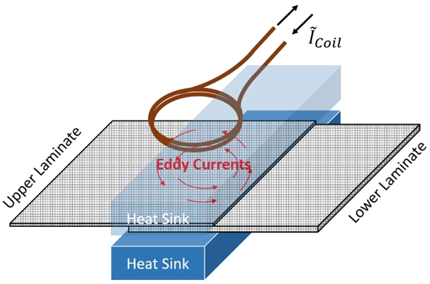
Basic setup for induction welding.

$\nabla \times \stackrel{\rightharpoonup }{E}=-\frac{\partial \stackrel{\rightharpoonup }{B}}{\partial t}$

1

$\stackrel{\rightharpoonup }{j}=\sigma \stackrel{\rightharpoonup }{E}$

2

${\dot{Q}}^{\mathrm{″\prime }}=\stackrel{\rightharpoonup }{j}\cdot \stackrel{\rightharpoonup }{E}=\stackrel{\rightharpoonup }{j}\cdot {\sigma }^{-1}\stackrel{\rightharpoonup }{j}$

3

where $\stackrel{\rightharpoonup }{E}$ is the electric field, $\stackrel{\rightharpoonup }{B}$ is the magnetic field, $\stackrel{\rightharpoonup }{j}$ is the electric current density, and $\sigma$ is the 3D electrical conductivity tensor.

The volumetric heat generation rate is proportional to the energy losses and, therefore, heating in the composite. ^3,4 The eddy currents in a layered composite are of a more complex nature (both in-plane and out-of-plane) than their equivalents in an isotropic material (mostly in-plane, expect near the edges). The generated heat will, locally, melt thermoplastic polymer allowing a cohesive bond to form between two TPC components.

As mentioned earlier, an advantage of induction heating is that it is a contactless, volumetric heating method, i.e. no contact is required between heating element and work piece. ⁵ This means that outer surfaces can be cooled either passively with heat sinks, or actively through air flow, while the composite laminates are being welded. The cooling allows the user to preserve consolidation and quality of the outer surfaces while melting the material only at the desired location, i.e. close to the interface between the two components; the weld zone.

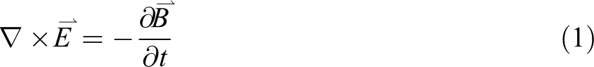
The heat generation within a laminate is governed by one, or a combination of the following three heating mechanisms, see Figure 2: (i) fiber heating; (ii) polymer heating; and (iii) contact resistance heating. ⁶ It is important to note that the dielectric polymer heating is neglected due to the relative low frequencies involved with induction welding process. ⁷

Figure 2.

Induction heating mechanisms (a) Joule based fiber heating, (b) Joule and/or dielectric polymer heating, (c) contact resistance heating.

• Fiber heating is the result of Joule losses due to the resistance of the fiber material. This loss is dependent on fiber diameter, fiber length, and resistivity ⁸ (Figure 2(a)).

• The space between fibers is filled with polymer. This polymer acts as a dielectric, but at the very small dimensions of the polymer volume between the fibers, the polymer also acts as a conductor of high but finite resistance ⁸ (Figure 2(b)). When an alternating magnetic field is applied to the laminate, an alternating potential difference or E-field is created between the differently oriented fibers in adjacent layers and Joule and dielectric losses may occur in the polymer. For very small separation distance between fibers, the electric field can become very strong (e.g. ${10}^6 \text{V}/\text{m}$ ), the associated induced currents could be a source of heating, however, this paper does not investigate this effect.

• The third heating mechanism is through fiber-to-fiber contact between fibers in adjacent plies and different in orientation angle (Figure 2©). At the points of contact, i.e. at the fiber junctions, temperature and pressure dependent resistance will arise, which can generate heat. ⁸

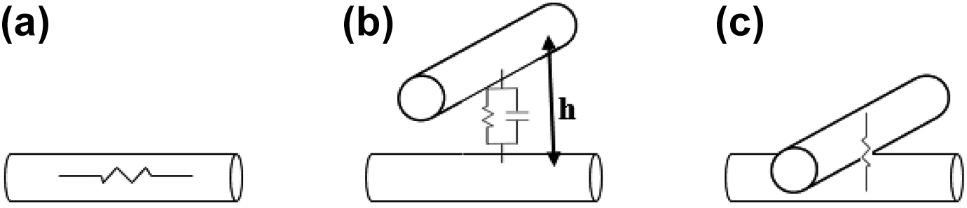
Based on the literature, two heating mechanisms have a significant contribution to the generated heat. ^{9 –14} designate contact resistance between fibers as the most dominant heating mechanism in the laminate. In the study by Kim et al. ⁹ the researchers cut strips of unidirectional tape and placed the strips in a square configuration as shown in Figure 3. A pancake coil was used to heat the configuration at constant power levels. The researchers concluded that because the maximum heating occurred at the junctions (indicated by J1, J2, J3, and J4 in Figure 3), the dominant heating mechanism must be due to the contact resistance between the $0°$ and $90°$ fiber directions, thereby ignoring possibilities of the heat to be cause by the change in fiber orientation at the junctions. In a different paper, ¹⁰ the same researchers reiterate that fiber contact is the dominant heating mechanism. Based on surface temperature measurement multiple papers ^{11 –13} have echoed that fiber contact is the driving heating mechanism and that Joule heating of the fiber is secondary to it.

Figure 3.

(left) configuration of unidirectional strips used in the study by Kim et al. ⁹ ; and (right) the heating profile measured.

The authors of this paper have in previous work ^{14 –16} used numerical simulations to counter that contact resistance is a dominant heating mechanism. Instead, Joule heating of the fiber and polymer are indicated to be the dominant heating mechanisms. ^{14 –16} The latter claim is supported by Lin et al. ¹⁷ and Mitschang et al. ¹⁸ as well.

Since there is no conclusive answer to which heating mechanism is dominant, the ANSYS Maxwell simulations described in this paper span a range of computational experiments aimed at the discovery of the dominating heating mechanism(s).

Numerical models

To investigate the effects of parameters such as the ply orientation, stacking sequence, fiber-to-fiber contact, fiber diameter, fiber-to-fiber spacing, presence of resin, etc. on the solid losses, which is proportional to the generated heat, a series of numerical models were created in ANSYS Maxwell. The solid loss (P) is calculated for each 3D volume (element) using

$P=\underset{V}{\overset{}{{\displaystyle \int }}}\frac{1}{{\sigma }_s}{J}^{2}dV$

4

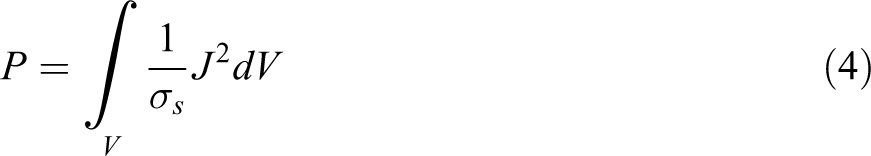
where J is the current density, $\sigma$ the conductivity of the volumetric element (a scaler in this case), and $dV$ is the differential volume. It is important to note that due to computational restrictions the number and size of the modeled fibers was kept to a minimum. The models, however, were still deemed representative to investigate which heating mechanism is dominant on the microscopic level. In addition, the plies were not modeled as continuous material, but as a set of individual fibers (see Figure 5). The numerical work repeated here was part of a M.S. thesis work. ¹⁹

No resin, vacuum system models

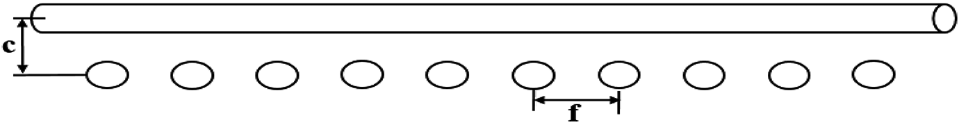
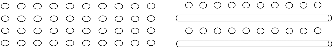
In the first series of simulations a square conductive copper coil (length and width of 25-mm, and height of 5.5-mm) was placed 6-mm (measure from the bottom of the coil) above the laminate, see Figure 4. The coil cross-section had a width, a, of 4.5-mm and height, b, of 5.5-mm. The individual fibers were modeled as cylinders of length 25-mm and diameter 0.4-mm and meshed using tetrahedral elements. The fiber-to-fiber distance, f, and the distance between the different layer, c, were 2.7-mm and 0.8-mm respectively. It is important to state that both f and c were measured from center-to-center as is shown in Figure 5. The relative permeability and relative permittivity were set to 1, the conductivity of carbon fibers was assumed to be $65000$ S/m, ²⁰ the coil was excited at a frequency of 292-kHz and AC of $500$ -A.

Figure 4.

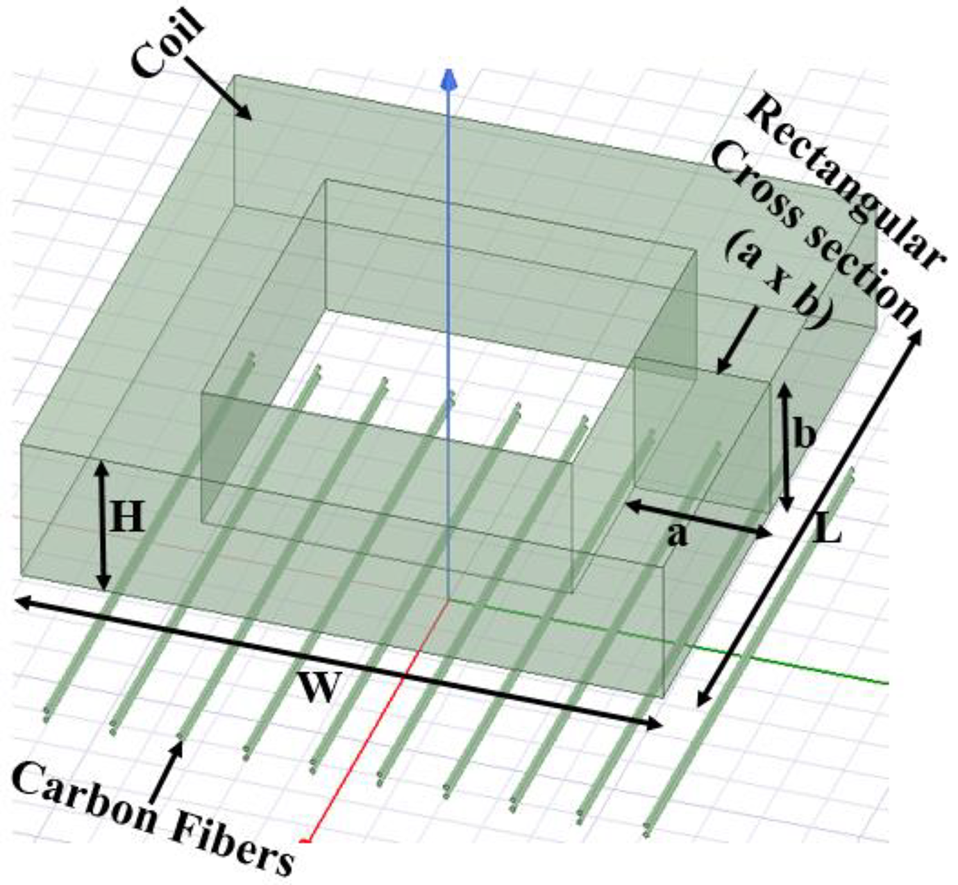
Simulation model with two layers of carbon fibers oriented in one direction.

Figure 5.

Two layers; 0’s and 90’s fiber orientation (front view).

It is important to state that in this paper we use the terms layer(s) to indicate the different set of fiber layer(s). Four different layers of individual fibers representing laminates orientated at: (i) $\left[0\backslash 0\right]$ ; (ii) $\left[0\backslash 90\right]$ ; (iii) $\left[0\backslash 0\backslash 0\backslash 0\right]$ ; and (iv) $\left[0\backslash 90\backslash 0\backslash 90\right]$ , with no resin system were modeled. The solid losses were calculated and are shown in Table 1. For the first case, $\left[0\backslash 0\right]$ , the solid loss was calculated to be $4.91\cdot {10}^{-3}$ -W, because there was no resin present and the fibers were not in contact with each other, the solid loss must have been caused by Joule heating of the fibers alone, recall Figure 2(a). The calculated solid loss is low due to the limitation in size and number of the carbon fibers used in the simulation as mentioned earlier. In a realistic case, the fibers have an approximate diameter of 10- $\mu$ m, and at a fiber volume fraction of 65% this would result in 8260-fiber/ ${\text{mm}}^2$ , while in this model the density of fibers was 20-fiber/ ${\text{mm}}^2$ . For the second case, $\left[0\backslash 90\right]$ , the solid loss was $5.32\cdot {10}^{-3}$ -W. The solid loss was, again, attributed due to Joule heating in the fiber direction because there was no resin or contact between fibers. Comparing the two cases, one notices an increase in solid loss, this was attributed to the change in conductivity (and thus resistivity) between the fiber layers, thereby increasing the solid loss.

Table 1.

Solid loss comparison for different laminates.

Simulation models	Solid loss ( $\cdot {10}^{-3}W$ )
$\left[0\backslash 0\right]$	4.91
$\left[0\backslash 90\right]$	5.32
$\left[0\backslash 0\backslash 0\backslash 0\right]$	8.73
$\left[0\backslash 90\backslash 0\backslash 90\right]$	9.91

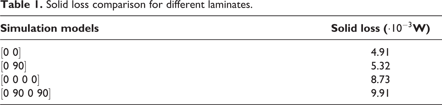
In the third and fourth case the number of layers was increased from two to four, see Figure 6. The layer orientations were $\left[0\backslash 0\backslash 0\backslash 0\right]$ and $\left[0\backslash 90\backslash 0\backslash 90\right]$ , respectively. It is important to note once more that all other parameters were kept the same. The calculated solid loss for the third case, $\left[0\backslash 0\backslash 0\backslash 0\right]$ , was $8.73\cdot {10}^{-3}$ -W, which is approximate double the value found in the first case, $\left[0\backslash 0\right]$ . Comparing all zero-degree cases it can be concluded that the solid loss is proportional to the number of layers. The solid loss did not exactly increase by a factor of 2 however, and this was due to the fact that the EM fields are diminishing with increasing distance from the coil, therefore, the bottom two layers experience a lower EM field than the top two layers.

Figure 6.

Four layers laminates; (left) [0\0\0\0], and (right) [0\90\0\90].

For the fourth case, $\left[0\backslash 90\backslash 0\backslash 90\right]$ , the solid loss was $9.91\cdot {10}^{-3}$ -W, this was an increase compared to case-2, $\left[0\backslash 90\right]$ , but not as significant as the increase seen between case-1 and case-3. Based on given numerical simulations and the results from case-1 to case-4 it was concluded that:

induction heating of non-touching carbon fibers in vacuum works better with orthogonal layers of fibers than with layer of identical direction fibers;

doubling the number of layers resulted in an almost proportionally increase of the solid loss when all layers are orientated in the same direction;

doubling the number of layers for orthogonal layers (case-4 compared to case-2) the increase in solid loss is less significant.

Heat at interface of layer orientation change

The second series of simulations focused on the hypothesis that the generated heat is concentrated at the interface between two layers which have different orientation angles. To examine the hypothesis additional $90°$ and $0°$ layers are added to a $\left[90\backslash 0\right]$ laminate to obtain different models while the fiber orientation of the layers adjacent to the interface remained the same; (if) $\left[90\backslash 0\right]$ ; (ii) $\left[90\backslash 90\backslash 0\backslash 0\right]$ ; (iii) $\left[90\backslash 90\backslash 90\backslash 0\backslash 0\backslash 0\right]$ ; etc. It must be noted that the distance from the coil to the $\left[90\backslash 0\right]$ -interface, the welding plane, was kept the same for all models. The $90°$ -layers layers were added on top and the $0°$ -layers on the bottom. If heat generation increase is less than proportional to the number of layers added, it might be concluded that heating is concentrated at the interface of layers with different orientation. If this hypothesis is correct, then simulations may be limited to interface layers only instead of an entire laminate. For these models the fibers were not in contact and there was no resin present. The diameter and length of the carbon fibers were 0.07-mm and 5-mm, respectively, and the center-to-center distance between any adjacent (in-plane) fibers within an layer was 0.014-mm, the (out-of-plane) distance between the two layer was also kept as 0.014-mm. At last the conductive coil was placed at 6-mm above the welding plane, see Figure 7.

Figure 7.

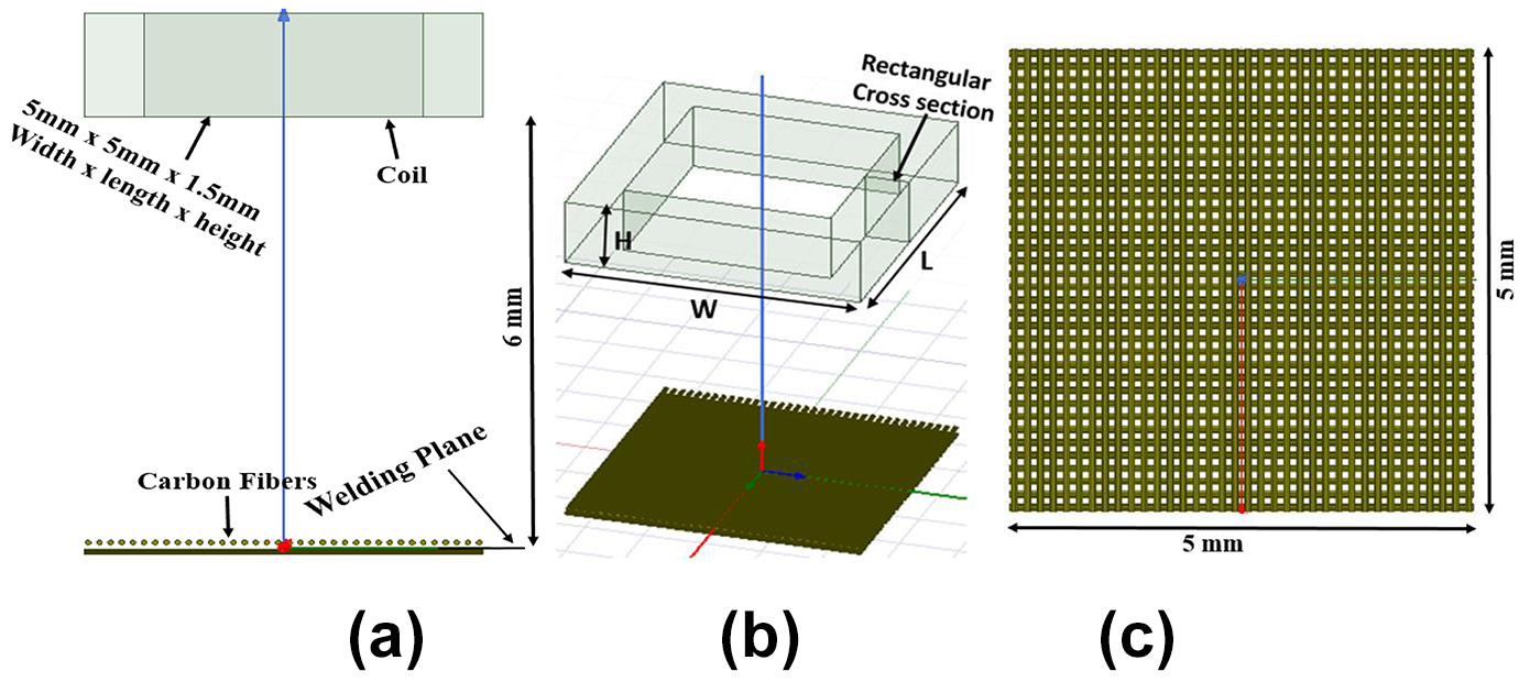
Hypothesis simulation model (a) side view, (b) trimetric view, (c) top view.

To limit computational resources required, the dimensions of the layers and coil were reduced. The fiber layers were reduced to 5-mm and the coil was reduced to a square of 5-mm and cross-section of 1.5-mm by 0.75-mm, see Figure 6. Even with the reduced dimensional parameters, no convergence was obtained, because the number of tetrahedra required to mesh the problem exceeded the available computational resources. Therefore, two cross-sectional geometries were considered as alternative for the circular one, see Figure 8, were examined to reduce the total number of elements required to mesh the entire model.

Square fibers while maintaining the same cross-sectional area by $A=r/0.565$

Polyhedron fibers instead of using a cylindrical shape of the cross-section. A circle was created using 12 small line segments as shown below.

Figure 8.

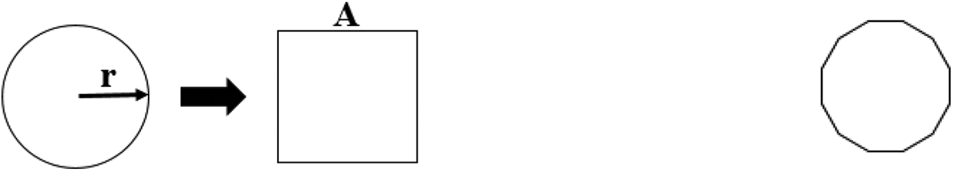
Alternative cross-sectional fiber geometries; (left) square; and (right) polyhedron.

The two alternative fiber cross-sectional geometries were compared with the initial cylindrical shape for an orientation $\left[0\backslash 90\right]$ layer configuration. The solid loss and the number of elements to mesh the model were used to determine which was the best option. The results in Table 2 show the polyhedron required the least number of elements and deviated the least form the solid loss calculated using cylindrical fibers. Therefore, for the remainder of this study polyhedron fibers were used. It is important to state that the solid loss did deviate 25% from the cylindrical shaped fibers, however, this a comparative study and as long the same cross-sectional fiber shape is used in all models any conclusion drawn remains valid.

Table 2.

Comparison of three different cross-sectional fiber shapes.

Fiber shape	Solid loss	Tetrahedra	No. of fibers	Converged
Cylinder	1.1459E−8	1986415	72	Yes
Square	6.6528E−9	249702	76	Yes
Polyhedron	8.8997E−9	190708	72	Yes

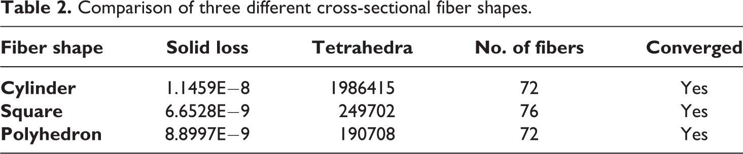
Using polyhedron fibers, the number of $90°$ - and $0°$ -layers was increased from 1 to 17. Recall that the interface, the welding plane, remained at the same distance from the coil in each model. The solid loss did increase with the increase in number of layers; however, the increase was not linear as is shown in Figure 9. The hypothesis at the start of this section is therefore is not valid.

Figure 9.

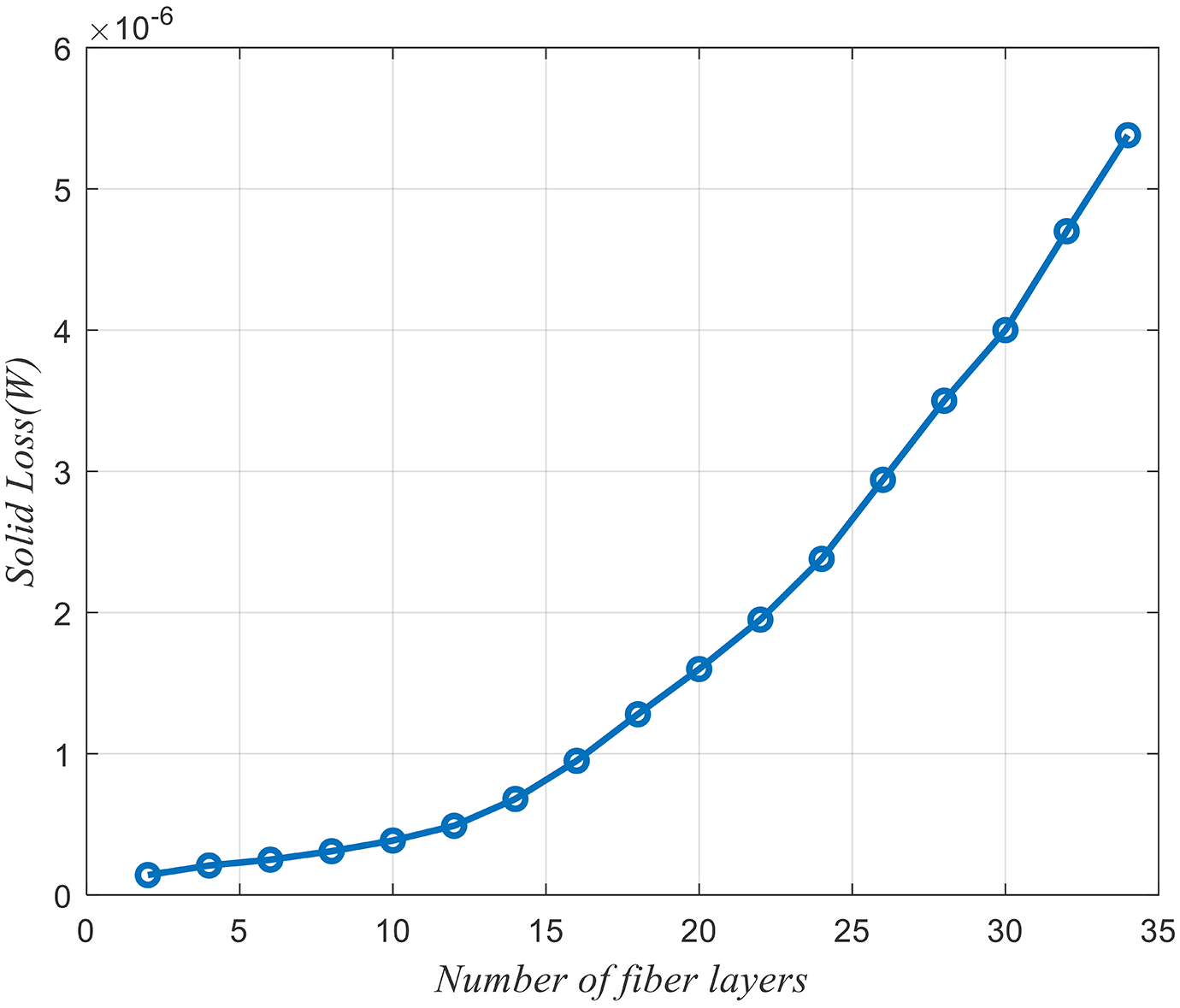
Solid loss as a function of total fiber layers in a 0/90 ply laminate. No of layers on the horizontal axis is the sum of the layers in the 0 and the 90 plies.

Heat dominated by the EM fields through the resin system

The next series of simulations and models was focused on the effect of the presence of a resin system on the solid losses. To investigate the effects of resin, two major changes were made to models compared to previous models.

The cross-sectional dimensions of the fibers and the distances between the fibers are reduced to values seen in real composites

Resin is added between fibers

Based on a fiber volume fraction of 65% and a fiber diameter of 7- $\text{μm}$ the size of each fiber/resin-cell was determined to be 7.7- $\text{μm}$ , see Figure 9. In these models the square coil was replaced by a circular coil with diameter of 250- $\text{μm}$ , the coil was placed 600- $\text{μm}$ above the laminate and it was excited at a frequency of 292-kHz and at an AC of 500-A, see Figure 10.

Figure 10.

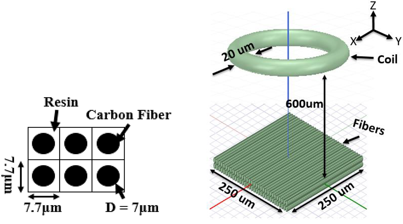
Simulation model parameters; (left) microscopic scale parameters; and (right) global scale parameters.

To investigate the effect of the resin on the solid loss, two layer configurations were used, (i) $\left[0\backslash 0\right]$ ; and (ii) $\left[0\backslash 90\right]$ . It is important to state that both models were evaluated with and without resin so conclusions regarding the presense of a resin could be made.

Prior to this series of simulations the effect of bulk resin conductivity values was investigated. For this intermediate research step the size of the major and minor radius of the coil was set to 50 $\mu$ m and 15 $\mu$ m, respectively. The resin conductivity was changed from 1 to ${10}^{-8}$ , and the corresponding solid losses are show in Table 3. Based on the result in Table 3 the solid losses converged when using the bulk resin conductivity ${10}^{-6}$ S/m or lower.

Table 3.

Resin conductivity value effect on solid losses.

Conductivity (S/m)	Solid loss .10−13 (W)
1.01	15.93
1	15.79
0.1	3.12
0.01	1.84607
0.001	1.84921
0.0001	2.8612
0.00001	5.83
0.000001	1.68
0.0000001	1.67
0.00000001	1.667

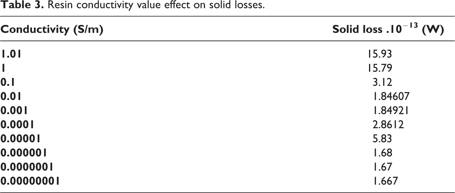
It is important to note when using a bulk resin conductivity of 10⁻⁶ S/m (or lower) did not yield any increase in solid losses compared to the case without the presence of resin (see Table 4). This, however, counteract what is seen experimentally in which the heat generation significantly increases when there is a change in layer orientations compared to only unidirectional laminates, e.g. $\left[0\backslash 0\right]$ compared to $\left[0\backslash 90\right]$ . To correlate simulation results to experimental observations an artificial resin conductivity value was used, which in this case was 1.01 S/m.

Table 4.

Comparison of results with and without conductive resin.

Simulation models	Resin	Solid loss ( $\cdot {10}^{-14}$ -W)	Factor
$\left[0\backslash 0\right]$	No	235	1
$\left[0\backslash 90\right]$	No	285	1.2
$\left[0\backslash 0\right]$	Yes (1.01 S/m)	561	2.4
$\left[0\backslash 90\right]$	Yes (1.01 S/m)	2690	11.4
$\left[0\backslash 0\right]$	Yes (10−8 S/m)	235	No change with respect to ‘no resin’ case
$\left[0\backslash 90\right]$	Yes (10−8 S/m)	285	No change with respect to ‘no resin’ case

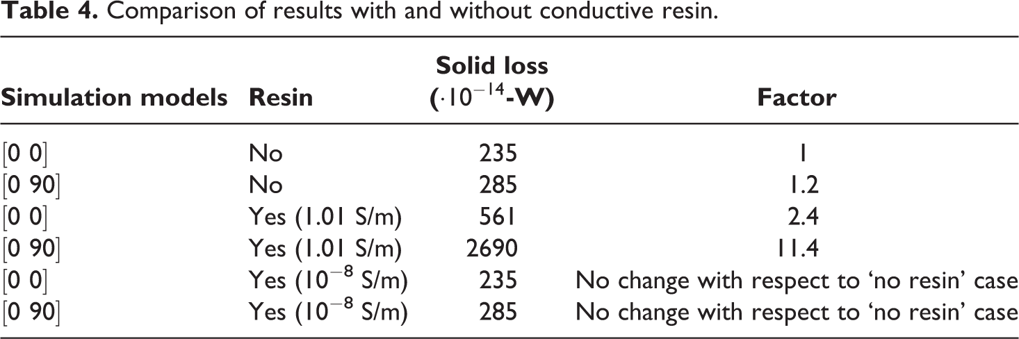
The calculated solid losses for the two laminates with and without resin are collected in Table 4. It can be seen that the presence of resin increased the solid losses significantly for both layer configurations when compared to their corresponding no-resin case. In addition, a cross-ply layer, $\left[0\backslash 90\right]$ , experienced a higher solid loss than a unidirectional layer, $\left[0\backslash 0\right]$ . From the cases without resin, see section II.A as well, it was concluded that Joule heating of the fiber was a dominant heating mechanism for induction welding. The two cases with resin showed that the presence of resin increased the solid losses significantly. The presence of a resin enables the eddy currents across fiber and resin, instead of only very small eddy currents at the fiber level. Joule heating of the polymer (Figure 2(b)) is, therefore, also a significant heating mechanism for induction welding.

The effect cross-sectional distribution of fiber and resin on the solid losses

The last study investigated the effect of resin distribution in the cross-section of layer on the solid losses. In some prepreg there is a clear resin rich layer on top of the fibers, while other prepreg shows a more homogeneous distribution of fibers through the thickness of the layer. The distance between two fiber layers was, therefore, varied to study the effect of the relative position of the fibers, see Figure 11.

Figure 11.

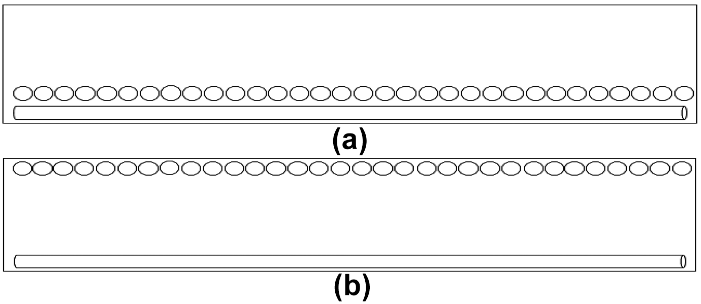
Simulation models (a) spacing of 0.5µm between the layers, (b) spacing of 23.5µm between the layers.

For this series of simulations, the distance between the layepors was varied from 0.5- $\text{μm}$ to 24- $\text{μm}$ , while for the previous simulation the distance was kept at 0.7- $\text{μm}$ . The total thickness of the was kept the same at 38.2- $\text{μm}$ . Except the distance between layers, all other model parameters were identical as in section II.C.

The effect effect of the relative position of the fiber layers on the solid losses is shown in Figure 12. A reduction in distance between fiber layers resulted in higher solid losses. This clearly establishes the fact that the loss is governed by the electric field in the resin between the fiber layers. Recall that when there was no resin the solid loss three orders of magnitude lower (see Table 4).

Figure 12.

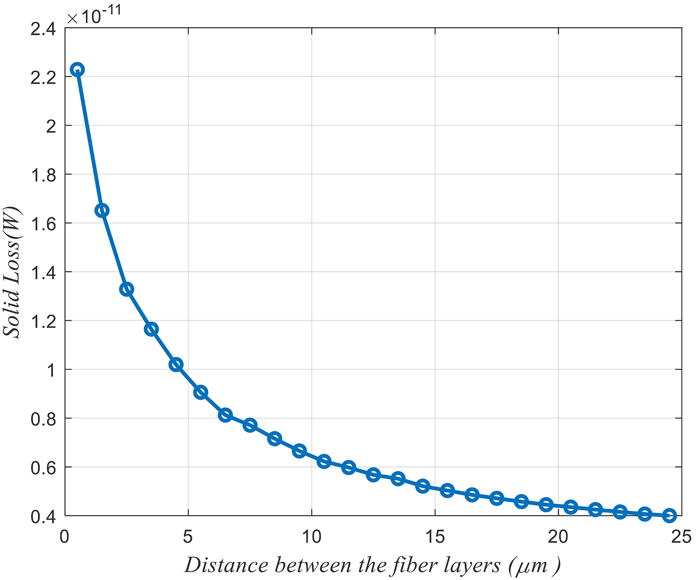
Plot of solid loss as a function of distance between fiber layers.

To explain Figure 12, let us consider a fiber in layer 1 which contains induced current I ₁ and the fiber below it contains induced current I ₂. Depending on the distance between the fibers the electric field created by these induced currents will vary. Note that the currents I ₁ and I ₂ are also a function of their distances and material around them. However, for a simplistic case if we assume that I ₁ and I ₂ are not changing significantly the electric field will significantly intensify as the distance between the fibers decrease. The intense electric field solid losses (resulting from EM energy absorption or polymer Joule heating) will increase since they are proportional to the square of the magnitude of the root mean square electric field. This situation is analogous to a two-wire power line. The shorter the distance between the lines, the larger is the electric field between them. ²¹ Furthermore, the effect is more than proportional, meaning that induction heating will be very sensitive to irregularities in fiber distribution over the cross-section of individual plies and laminate.

Effect of ply orientation on solid losses for three layer-to-layer configurations

The last series of analysis repeated the simulations of section II.D with an increased resin layer of thickness 72.8- $\text{μm}$ using three different stacking sequences for three different layer-to-layer distance values, see Figure 13. The stacking sequences evaluated were: (i) $\left[0\backslash 90\right]$ ; (ii) $\left[0\backslash 45\right]$ ; and $\left[45\backslash 90\right]$ , while the layer-to-layer distance evaluated were 0.7- $\text{μm}$ , 21- $\text{μm}$ and 42- $\text{μm}$ .

Figure 13.

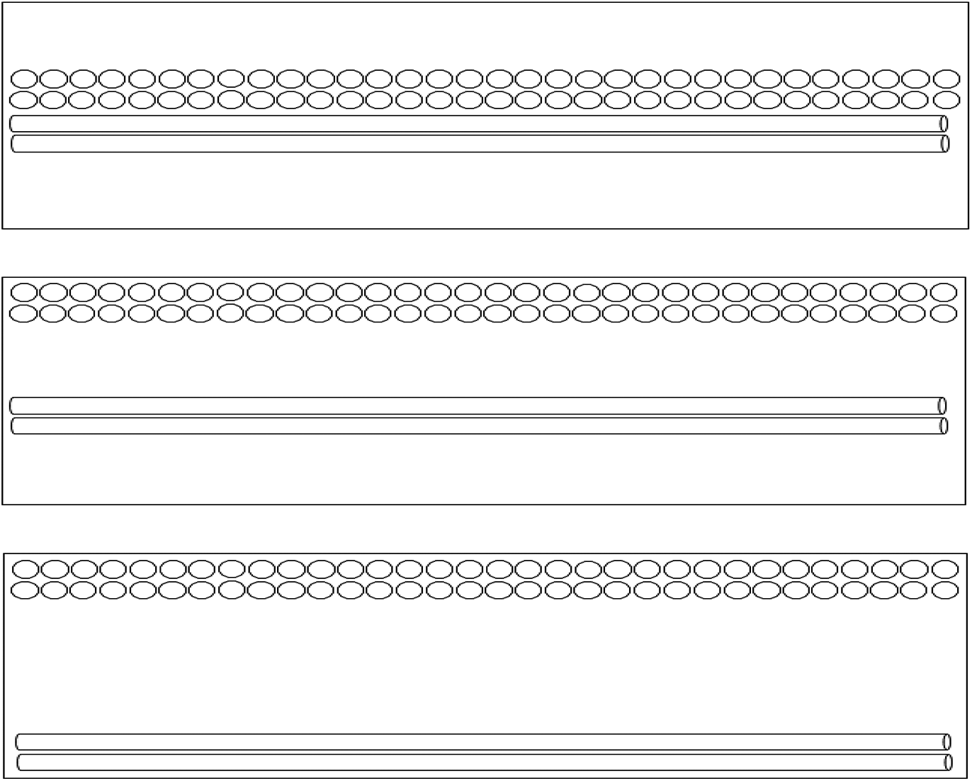
Three different arrangement with 0’s and 90’s plies.

The results in Table 4 show that the $\left[0\backslash 90\right]$ configuration had the highest solid loss compared to the other configurations for all layer-to-layer distance values. For all configurations, solid loss is decreasing with increasing gap size. More resin and an increased distance between layers reduced the electric fields due to the increased distance between the induced currents. Resulting in a reduction the currents in the polymer.

Table 5.

Results comparison for all nine-simulation models.

Solid loss ( $\cdot {10}^{-12}W$ )
Layer distance [ $\mu m]$	$\left[0\backslash 90\right]$	$\left[0\backslash 45\right]$	$\left[45\backslash 90\right]$
0.7	31.87	13.22	13.24
21	10.71	7.85	7.93
42	8.23	6.95	7.07

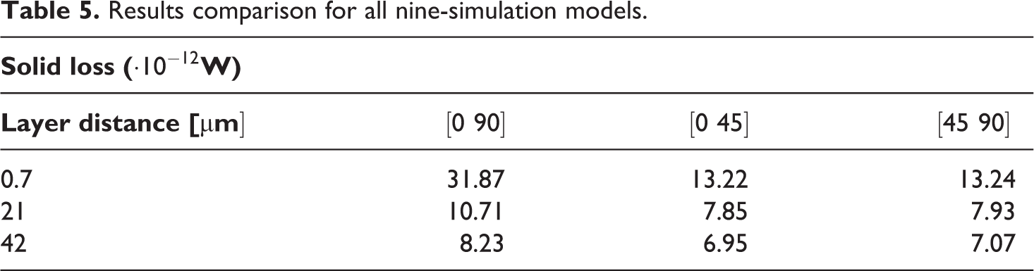
Furthermore, it can be concluded, the parameters that affect the solid loss most are the difference in fiber orientations between adjacent plies and the volume in between the layers. Adjacent $0°$ and $90°$ layers are good for induction heating but normally not favored for mechanical properties. Fortunately, induction heating of $0°$ and $45°$ adjacent layers work as well, see Table 5.

Conclusion

Induction heating of thermoplastic composites was studied using simulations in ANSYS Maxwell. Given that practical carbon fiber composite laminates contain millions of fibers in proximity which practically are immersed in resin, it is impractical and probably impossible to develop a large representative simulation model. Thus, simulation models of smaller specimens were developed consisting of limited numbers of fibers and limited amounts of resin within a small volume. Furthermore, to facilitate the simulation, the fibers were modeled as polyhedrons instead of circular cylinders reducing the accuracy by 25%, but the quantitative validity of the results were assumed to be good. The results obtained from the simulations indicate that fiber orientation is a dominant parameter that affect the solid losses generated during induction welding. However, the effect of the presence of resin could not be verified, because using a bulk resin conductivity value of ${10}^{-8}$ S/m yielded no change in solid losses compared using no resin at all. This, however, does not correlate with experimental observations. Therefore more research regarding properties (electrical conductivity, crystallinity, moisture level, etc.) for very thin resin layers (e.g, order magnitude $7\mu$ m) must be conducted before any conclusion regarding the effect of the presence of resin on the solid losses can be made. Note that the actual temperature increase in the material is also a function of exposure time which is not included in this study.

It was found that simulation models containing layers of fibers oriented in $0°$ and $90°$ orientation yield significantly higher solid loss than layers of fibers oriented in the same direction. It was observed that inclusion of polymer resin in the models yielded far greater solid loss compared to no-resin cases, especially for very small separation distances between fiber layers. For the case with $0°$ , $90°$ oriented layers, the inclusion of resin increased the solid loss by almost a factor of 200. It became clear that the presence of the resin is needed to obtain enough solid losses, and therefore heating. It is understood that the intense electric fields caused by the induced currents in the fibers in the different layers intensify solid loss in the entire specimen, especially when the layer-to-layer distances are small and there is a resin system with reasonable conductivity present.