Control of the through-thickness temperature distribution in carbon composite aerospace parts during induction welding

Abstract

The increasing content of thermoplastic composites in the aerospace industry requires the application of new joining technologies. Their main assembly advantage is rivetless joining, which needs to be examined in greater detail in order to compensate the higher costs of these materials. Induction welding is already used in aerospace industry and shows a high potential for the application in helicopter manufacturing. In order to implement this technology in serial production, the main requirement is to determine and control the process temperature distribution. A wide range of literature describing various approaches that characterize the aforementioned temperature distribution exists. Although all approaches validate their findings by temperature measurement on the surfaces of their parts, their results seem inconsistent due to different results. In this article, a new approach is presented and validated by interlaminar temperature measurement. Based on this new approach, for induction welding, effects that are not yet described are discussed. Hereby, cooling of the surface by air jets is investigated as a mean to influence the thermal effects of the induction welding process.

Introduction

Increasing requirements concerning cost savings, efficiency, performance, and quality lead to an increasing content of carbon fiber–reinforced thermoplastic composites (CF-TPCs) in helicopter manufacturing. In contrast to thermoset composites weight saving, rivetless joining technologies like fusion bonding can be used. ¹ With this technology, entirely consolidated thermoplastic composite parts can be joined only by means of heat and pressure and without any additives. ^{1 –4} The induction welding technology, for example, which is already utilized for the joining of thermoplastic parts in wing aircraft, is based on this technology. ⁵ However, a wide range of requirements must be fulfilled for qualification in order to implement this technology for aerospace applications such as helicopter manufacturing. The main challenge is the process design as it is required to control the temperature distribution within the component. This will ensure that the degradation temperature is not exceeded, the welding temperature in the welding zone is reached, and that the surfaces do not melt (shown in Figure 1). In particular, Augh et al. ⁶ carry out investigations on the issue of degradation during the induction welding process. One of the main factors to prevent the described thermal degradation ⁶ and hence the reduction of the mechanical properties of the components is the through-thickness temperature distribution. Its knowledge enables to guarantee the successful realization of the welding without needing downstream quality insurance. Due to the high number of factors influencing the induction welding process, it is currently not possible to simulate the induction heating of arbitrary composite layups and designs. ³ Many different theories about the temperature distribution have been published. ^{2,7,8 –12} The theories of Rudolf et al., ² Moser, ³ Miller et al., ⁸ Kim et al. ⁹ , Yarlagadda ¹⁰ , and Fink et al ^11,12 consider the temperature distribution in carbon fiber–reinforced thermoplastics. Vrana’s studies ⁷ refer to nickel alloys and Iwashita et al.’s studies ¹³ examine copper foils. Miller et al.’s theory ⁸ states that the heating in thickness direction is uniform, which is then used by Rudolf et al. ² to measure the temperature on the upper and lower surfaces. For thin shells, Rudolf et al. reveal that the skin effect has no significant influence on the heating. ² Moser ³ measures the surface temperatures with thermal imaging. In contrast to Rudolf et al. and Miller et al., ^{2 ,8} he measures a temperature decrease from the top to the bottom surface and assumes an exponential decrease in the temperature. Further investigations of Vrana ⁷ and Iwashita et al. ¹³ show a thickness-dependent temperature distribution as well (see Table 1). The main drawback of these theories is their validation that is based on the measurement of the surface temperatures. In summary, the temperature distribution in thickness direction needs to be measured and a new theory must be developed, since the existing theories are inconsistent. Owing to the inhomogeneity of the materials, the finite element meshes should be on fiber and matrix level; otherwise, the heat simulation cannot predict the heat distribution in detail. ¹⁴ The aim of this research is to measure the temperature between the individual layers of the laminate. Based on these results, a more detailed process model is developed and the influence of optimization approaches is shown. In a first step, a 1D-approach is developed and validated on specimens with varying thicknesses. To influence the temperature distribution, the surfaces are experimentally cooled by an air jet with varying temperatures and volumes.

Figure 1.

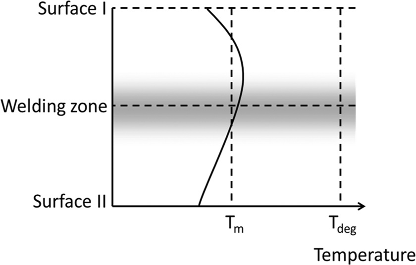
Targeted temperature distribution.

Table 1.

Theories about the temperature/current density distribution in thickness direction during the induction heating process.

Theory	Frequency (inductor geometry)	Measuring technology	Material	Specimen thickness (xs ) (dependent on skin depth (δS))	Temperature distribution (theoretical)
Miller8	450 kHz (double D)	melting point of three stacked laminates	PEEK/APC-2 graphite fiber tape; [0°; +45°; −45°; 90°]6 s	4.2 mm 0.26 xs /δS	uniform
Rudolf2	650–1000 kHz	thermal camera	PPS/CF Satin 5H	2 mm 0.43 xs /δS	uniform
Vrana7	360 kHz	thermal camera	nickel alloy	5 µm 0.25–2 xs /δS	increasing temperature with decreasing material thickness (0 < xs < 4 × δS); for thin structures (xs < δS) approximately uniform temperature distribution
Moser3	400 kHz	thermal camera	PEEK and PPS; CF Satin 5 H, 3 k, 285 g m−2	2 mm 0.43 xs /δS	linear decrease from the upper side to the lower side
Iwashita13	150 MHz	only simulation	copper foil	5 µm 0.92 xs /δS	parabolic for xs < δS

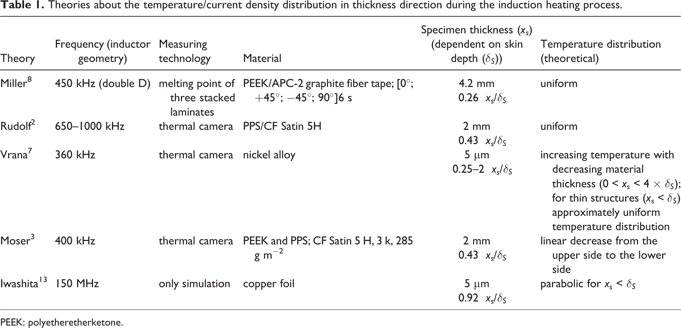
PEEK: polyetheretherketone.

Background and objectives

When preparing a process qualification of the induction welding process, the main challenge is the calculation and the control of the through-thickness temperature distribution. The aim is to prevent overheating of the laminate (degradation), an insufficient melting degree in the welding zone (no bonding) and melting of the top layers (insufficient crystallinity, varnishability, or delamination). An in-line quality assurance should guarantee a predefined temperature distribution by measuring or calculating the interlaminar temperature profile. As temperature sensors cannot be integrated in serially produced parts, only a measurement of the surface temperature is possible. Based on these results, the temperature distribution has to be calculated. For a surface varnish without pretreatment, the top layers must not melt while still reaching the welding temperature in the welding zone. The following objectives are therefore derived:

development of a validated model for calculating the temperature distribution in thickness direction, and

reaching a targeted temperature distribution by cooling the surface (see Figure 1).

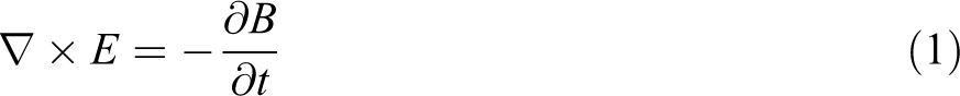
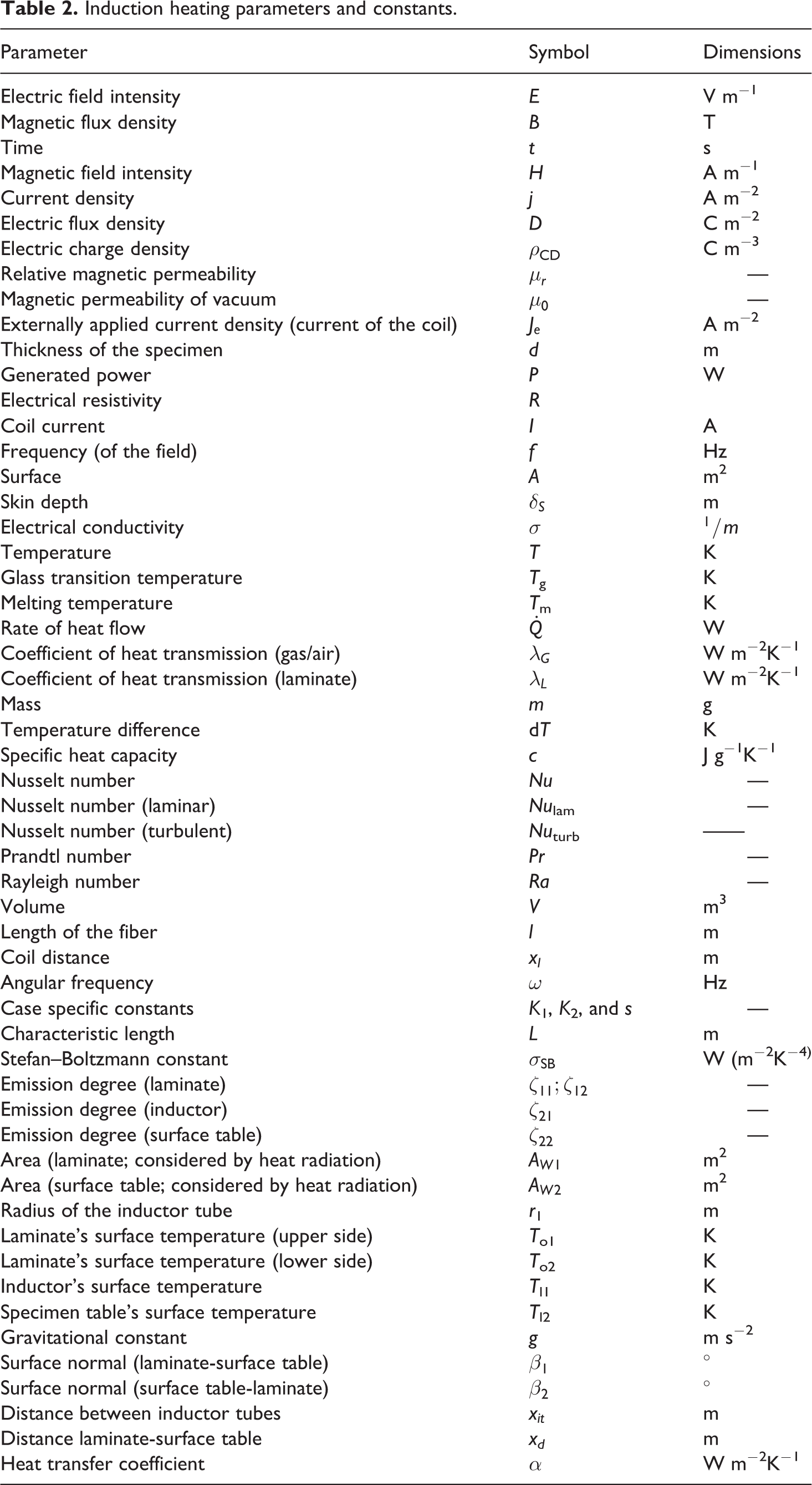
Faraday showed that a changing magnetic field produces a changing electric field and vice versa. The relation was modeled by Clerk Maxwell applying Faraday’s law (equation (1)). ¹⁵ The three other Maxwell equations are Gauss’s law (equation (3)), Gauss’s law for magnetism (equation (4)), and Ampère’s circuital law (equation (2)). ¹⁵ The symbols used in the following equations are explained in Table 2.

$\nabla \times E=-\frac{\partial B}{\partial t}$

1

$\nabla \times H\hspace{0.17em}=\hspace{0.17em}j\hspace{0.17em}+\hspace{0.17em}\frac{\partial D}{\partial t}$

2

$\nabla \cdot \hspace{0.17em}D=\hspace{0.17em} {\rho }_{cd}$

3

$\nabla \cdot B\hspace{0.17em}=\hspace{0.17em}0$

4

Table 2.

Induction heating parameters and constants.

Parameter	Symbol	Dimensions
Electric field intensity	E	V m−1
Magnetic flux density	B	T
Time	t	s
Magnetic field intensity	H	A m−1
Current density	j	A m− 2
Electric flux density	D	C m− 2
Electric charge density	ρ CD	C m− 3
Relative magnetic permeability	μr	—
Magnetic permeability of vacuum	μ 0	—
Externally applied current density (current of the coil)	Je	A m− 2
Thickness of the specimen	d	m
Generated power	P	W
Electrical resistivity	R	Ω
Coil current	I	A
Frequency (of the field)	f	Hz
Surface	A	m2
Skin depth	δS	m
Electrical conductivity	σ	$\raisebox{1ex}{$1$}\!\left/ \!\raisebox{-1ex}{$\text{Ω}m$}\right.$
Temperature	T	K
Glass transition temperature	T g	K
Melting temperature	T m	K
Rate of heat flow	$\dot{Q}$	W
Coefficient of heat transmission (gas/air)	λG	W m− 2K−1
Coefficient of heat transmission (laminate)	λL	W m− 2K−1
Mass	m	g
Temperature difference	dT	K
Specific heat capacity	c	J g−1K−1
Nusselt number	Nu	—
Nusselt number (laminar)	Nu lam	—
Nusselt number (turbulent)	Nu turb	——
Prandtl number	Pr	—
Rayleigh number	Ra	—
Volume	V	m3
Length of the fiber	l	m
Coil distance	xl	m
Angular frequency	ω	Hz
Case specific constants	K 1, K 2, and s	—
Characteristic length	L	m
Stefan–Boltzmann constant	σ SB	W (m− 2K−4)
Emission degree (laminate)	ζ11;ζ12	—
Emission degree (inductor)	ζ 21	—
Emission degree (surface table)	ζ 22	—
Area (laminate; considered by heat radiation)	A W1	m2
Area (surface table; considered by heat radiation)	A W2	m2
Radius of the inductor tube	r 1	m
Laminate’s surface temperature (upper side)	T o1	K
Laminate’s surface temperature (lower side)	T o2	K
Inductor’s surface temperature	T l1	K
Specimen table’s surface temperature	T l2	K
Gravitational constant	g	m s− 2
Surface normal (laminate-surface table)	β 1	°
Surface normal (surface table-laminate)	β 2	°
Distance between inductor tubes	xit	m
Distance laminate-surface table	xd	m
Heat transfer coefficient	α	W m− 2K−1

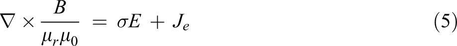
After a simplification of Ampere’s circuital law, the magnetic field intensity H and the magnetic flux density B can be coupled due to the frequency of the used electromagnetic field. Combining these equations with Ohm’s law gives ^{15 –17}

$\nabla \times \frac{B}{{\mu }_r{\mu }_0}\hspace{0.17em}=\hspace{0.17em}\sigma E\hspace{0.17em}+\hspace{0.17em}{J}_e$

5

Based on these equations, the magnetic flux density for infinite thick plates (thickness ≫ skin depth δ_S) can be calculated as ⁷

$H\left(x,t\right)\hspace{0.17em}=\hspace{0.17em}{H}_{0}Re\left(e^{-\sqrt{2i}\frac{x}{{\delta }_S}}{e}^{i\omega t}\right)$

6

which leads to a current density of ⁷

$j_z\left(x,t\right)\hspace{0.17em}=\hspace{0.17em}-\frac{\partial H\left(x\right)}{\partial x}\hspace{0.17em}=\hspace{0.17em}\frac{\sqrt{2}}{{\delta }_S}{H}_0\left(t\right)e^{\frac{i\pi }{4}}{e}^{-\sqrt{2i}\frac{x}{{\delta }_S}}$

7

For finite thick plates, the magnetic flux density is calculated as ⁷

$H\left(x,t\right)\hspace{0.17em}=\hspace{0.17em}{H}_{0}Re\left[\left(\frac{e^{-\sqrt{2i}\frac{x}{{\delta }_S}}}{1\hspace{0.17em}-\hspace{0.17em}{e}^{-\sqrt{2i}\frac{2d}{{\delta }_S}}}\hspace{0.17em}-\hspace{0.17em}\frac{e^{\sqrt{2i}\frac{x}{{\delta }_S}}}{1\hspace{0.17em}-\hspace{0.17em}{e}^{\sqrt{2i}\frac{2d}{{\delta }_S}}}\right)e^{i\omega t}\right]$

8

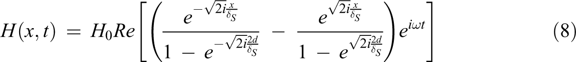
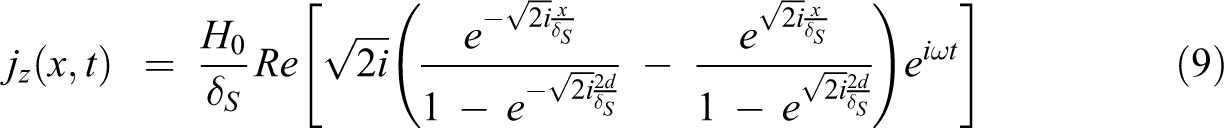
which leads to a current density of ⁷

$j_z\left(x,t\right)\hspace{0.17em}=\hspace{0.17em}\frac{H_0}{{\delta }_S}Re\left[\sqrt{2i}\left(\frac{e^{-\sqrt{2i}\frac{x}{{\delta }_S}}}{1\hspace{0.17em}-\hspace{0.17em}{e}^{-\sqrt{2i}\frac{2d}{{\delta }_S}}}\hspace{0.17em}-\hspace{0.17em}\frac{e^{\sqrt{2i}\frac{x}{{\delta }_S}}}{1\hspace{0.17em}-\hspace{0.17em}{e}^{\sqrt{2i}\frac{2d}{{\delta }_S}}}\right)e^{i\omega t}\right]$

9

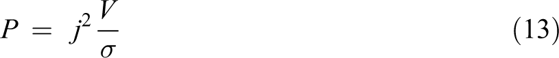
The resulting generated power can be given by ¹⁸

$P\hspace{0.17em}=\hspace{0.17em}{I}^{2}R$

10

with

$I=jA$

11

and

$R\hspace{0.17em}=\hspace{0.17em}\frac{l}{A\sigma }$

12

inserted in equation (10) leads to

$P\hspace{0.17em}=\hspace{0.17em}{j}^2\frac{V}{\sigma }$

13

with

$P\hspace{0.17em}=\hspace{0.17em}\frac{\Delta E}{\Delta t}$

14

results in

$\Delta E\hspace{0.17em}=\hspace{0.17em} j^2\frac{V}{\sigma }\Delta t$

15

with the energy equation

$\Delta E\hspace{0.17em}=\hspace{0.17em}c\hspace{0.17em}\cdot \hspace{0.17em}m\hspace{0.17em}\cdot \hspace{0.17em}\Delta T$

16

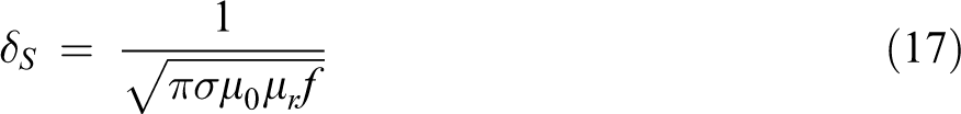
An alternating electromagnetic field with the frequency f is generated if an alternating current with the same frequency passes through a coil. Electrical eddy currents with the same frequency and therefore the power P is induced when a magnetically susceptible and electrically conductive material is placed in the vicinity of the coil and its alternating magnetic field. The relative magnetic permeability is one of the parameters determining the process. ¹⁸ This also influences the skin effect, which determines the skin depth δ_S. This depth describes the distance from the surface facing the inductor in which 63% of the magnetic intensity is converted into heat energy. ¹⁸

${\delta }_S\hspace{0.17em}=\hspace{0.17em}\frac{1}{\sqrt{\pi \sigma {\mu }_0{\mu }_{r}f}}$

17

In comparison with ferromagnetic metals with μ_r ≫ 1, the relative magnetic permeability of thermoplastic composites TPC materials is only μ_r ≈ 1. ¹⁸

In comparison with metallic parts, CF-TPCs are not homogeneous. ¹⁹ Two types of CF-TPCs are distinguished, either made of unidirectional tape or woven fabric. For both materials, the heating depends on the layup. A typical manufacturing process is fiber placement, in which the tapes are stacked with a defined orientation layer for layer. ²⁰ Arbitrary layups can also be manufactured and when producing structures out of woven fabrics, the thermoforming process is used. ²¹ For this process, fully consolidated plates with predefined layups are used as the semifinished product. ¹⁹

When current is induced into the fibers, the three principles, which are shown in Figure 2, cause induction heating. For isotropic or orthotropic layups, joule heating is the dominating heating effect. ¹⁰ As soon as the current flows through the fibers, the generated heat follows Joule’s law (equation (10)) ²² in addition to the energy being dissipated by contact resistance when two fibers are in contact. If the fibers are separated by a very thin layer of thermoplastic resin, they act as a capacitor. Consequently, heat is generated by dielectric heating. ¹⁰

Figure 2.

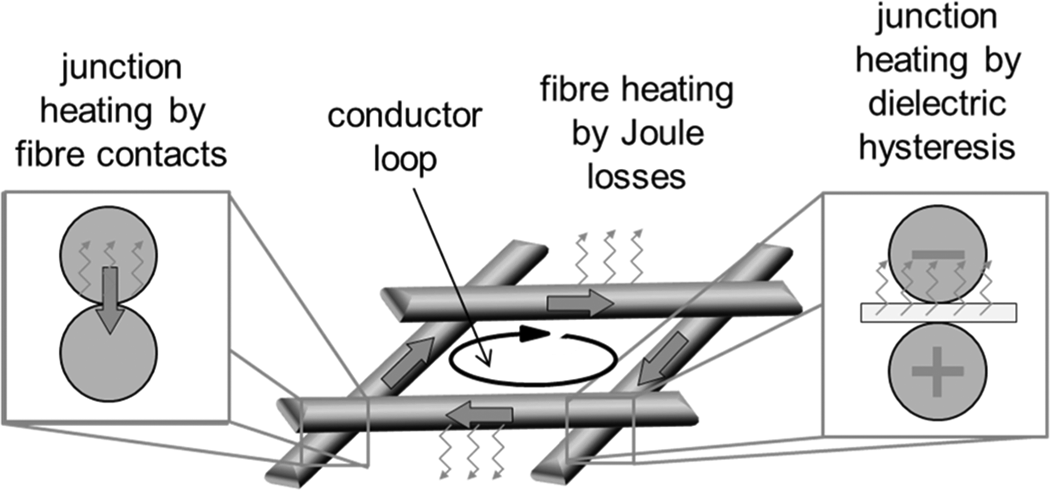
Induction heating mechanisms.

When the thermal energy exceeds the thermal losses in the setup, the temperature increases. For semicrystalline polymers, melting of the matrix occurs when exceeding melting temperature T _m, thereby creating a bond. ¹⁹ After reaching the defined degree of melting, the layup is cooled below T _g or T _m through the application of pressure. ^19,23

Depending on the layup, the parts will heat up differently in the electromagnetic field. According to Ahmed et al. ²⁴

a condition imposed on the material is that closed-loop circuits must be present for eddy currents to be induced. In the case of fibre-reinforced thermoplastics, closed-loop circuits in the form of a conductive network are produced through weaves or cross plies, for example.

Experimental setup

Heating experiments with different specimen thicknesses and different methods of surface-cooling are carried out. Cooling is realized by utilizing pressurized air with different temperatures and flow rates.

Materials and equipment

Unidirectional tapes (width of 1′′) with a polyetheretherketone (PEEK) matrix and HTA40 3K carbon fiber rovings are supplied by Toho Tenax Europe GmbH (Düsseldorf, Germany). The PEEK matrix is Vestakeep 200 from Evonik Industries AG (Germany). ²⁵

Thermocouples (type E) with a diameter of 0.13 mm are acquired from Omega (Germany). ²⁶ The temperature is measured with the thermo recorder Yokogawa DX1012 (Yokogawa Deutschland GmbH, Ratingen, Germany). The inductor has a pancake shape with a diameter of 25 mm and two circuits, manufactured from a 3-mm-thick copper wire. The induction was generated by a CEIA 400 kHz (PW3-32/400) generator (Ceia S.p.A., Arezzo, Italy). For measuring the flow rate, sensors SFAM-62 from FESTO (Esslingen, Germany) are used. The pressurized air is cooled down by cyclone tubes from EPUTEC Drucklufttechnik GmbH (Kaufering, Germany). ²⁷ A cyclone tube separates a compressed gas jet into a hot and a cold stream. The used pressurized air has a pressure of 0.6 MPa.

Specimen preparation

The manufacturing of the laminates is a two-step process. First, plies are formed on top of a stainless steel tooling plate, which is coated with a release agent, by tacking tapes with a soldering iron. In between the plies, thermocouples are inserted (see Figure 3). The stacking sequence is [0°/90°]s (4 plies), [0°/90°/0°/90°]s (4 plies), and [0°/90°/0°/90°/0°/90°/0°/90°]s (16 plies). Subsequently, the laminates are vacuum bagged and consolidated in an oven at 400°C for 1 h. The average heating rate is 4.5°C min⁻¹ and the average cooling rate is 2.3°C min⁻¹. The assembly used for consolidating is illustrated schematically in Figure 4. The breather is made of dry glass fabric. The vacuum bag and fixation tape are polyimide based, whereas the sealing tape is a high-temperature-resistant tacky tape. The final dimensions of the laminates are 400 × 100 mm². The specimens are manufactured with 4, 8, and 16 plies, and for each layup, six specimens are made.

Figure 3.

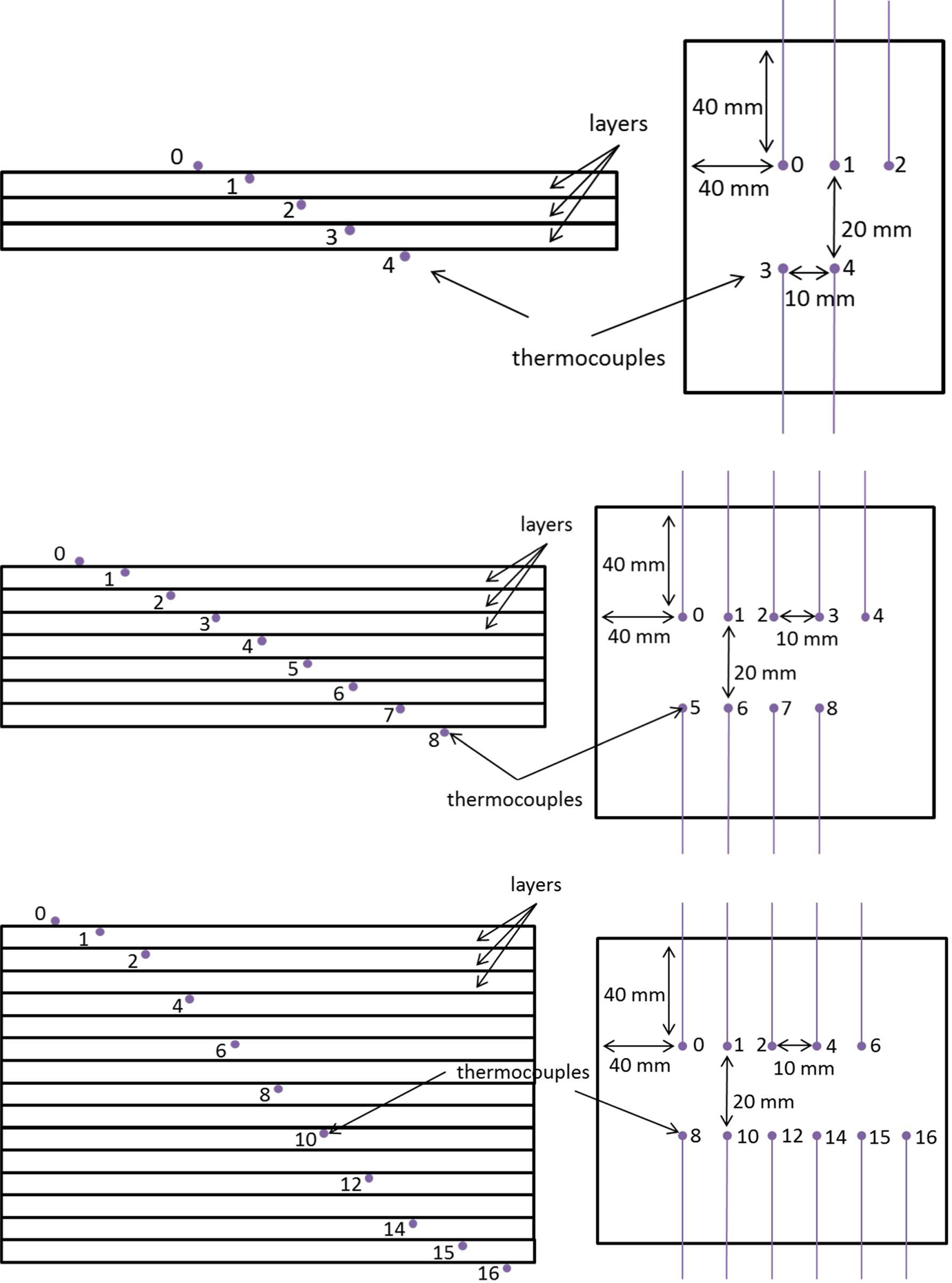
Positions of the thermocouples in a 4-, 8-, and 16-ply specimen (left: thermocouple positions in thickness direction; right: thermocouple positions in in-plane direction).

Figure 4.

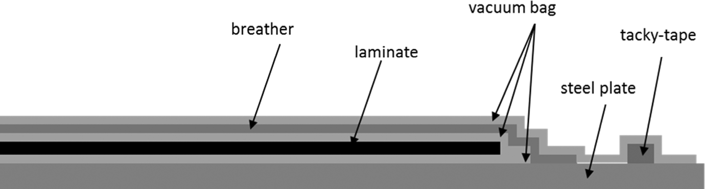
Assembly for consolidation of the laminates.

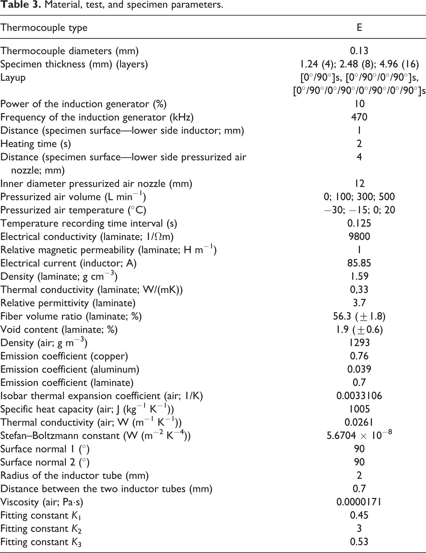
The thermal capacity diagram is shown in Figure 5. The remaining material data of the tapes and the laminates are given in Table 3. The good laminate quality (fiber volume ratio 56.3%; void content 1.9%) is comparable to other researches. ³ The high number of used thermocouples does not influence the quality of the results, because the in-plane thermocouple density is lower than 1 thermocouple per square centimeter.

Figure 5.

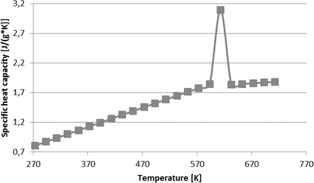
Specific thermal capacity.

Table 3.

Material, test, and specimen parameters.

Thermocouple type	E
Thermocouple diameters (mm)	0.13
Specimen thickness (mm) (layers)	1.24 (4); 2.48 (8); 4.96 (16)
Layup	[0°/90°]s, [0°/90°/0°/90°]s, [0°/90°/0°/90°/0°/90°/0°/90°]s
Power of the induction generator (%)	10
Frequency of the induction generator (kHz)	470
Distance (specimen surface—lower side inductor; mm)	1
Heating time (s)	2
Distance (specimen surface—lower side pressurized air nozzle; mm)	4
Inner diameter pressurized air nozzle (mm)	12
Pressurized air volume (L min−1)	0; 100; 300; 500
Pressurized air temperature (°C)	−30; −15; 0; 20
Temperature recording time interval (s)	0.125
Electrical conductivity (laminate; 1/Ωm)	9800
Relative magnetic permeability (laminate; H m−1)	1
Electrical current (inductor; A)	85.85
Density (laminate; g cm− 3)	1.59
Thermal conductivity (laminate; W/(mK))	0,33
Relative permittivity (laminate)	3.7
Fiber volume ratio (laminate; %)	56.3 (±1.8)
Void content (laminate; %)	1.9 (±0.6)
Density (air; g m− 3)	1293
Emission coefficient (copper)	0.76
Emission coefficient (aluminum)	0.039
Emission coefficient (laminate)	0.7
Isobar thermal expansion coefficient (air; 1/K)	0.0033106
Specific heat capacity (air; J (kg−1 K−1))	1005
Thermal conductivity (air; W (m−1 K−1))	0.0261
Stefan–Boltzmann constant (W (m− 2 K− 4))	5.6704 × 10−8
Surface normal 1 (°)	90
Surface normal 2 (°)	90
Radius of the inductor tube (mm)	2
Distance between the two inductor tubes (mm)	0.7
Viscosity (air; Pa·s)	0.0000171
Fitting constant K 1	0.45
Fitting constant K 2	3
Fitting constant K 3	0.53

Test setup and heating procedure

For every measurement, the CF/PEEK specimens are positioned beneath the coil on two aluminum blocks, and for every test, the tested thermocouple is placed under the coil as shown in Figure 6. In all tests, it is ensured that the coil position is aligned with the thermocouple position in the laminate. The surface to coil distance is about 1 mm and kept constant, the induction time is set to 2 s, and during the heating time of 2 s, the temperature is logged. After every measurement, the specimen is cooled down to room temperature. It is then repositioned under the coil and the measurement is repeated three times for every thermocouple which is integrated in the specimen. For each of the six specimens with the same ply number, these steps are repeated. For thermocouple position 1, for example, three measurements in the six specimens with the same ply number are done. The average temperature of these 18 measurements after 2 s is calculated and the results are plotted in the following charts. This process is repeated for the 4-ply, 8-ply, and 16-ply specimens and every parameter setup. The nozzle for blowing pressurized air is a polyurethane-tube with an inner diameter of 12 mm. The volume of the pressurized air is varied between 0 L min⁻¹ and 500 L min⁻¹ and the temperature between −30°C and 20°C. In order to minimize the temperature increase per time step, the power of the induction generator is set to 10%. During the heating process, the melting temperature is not reached and therefore no pressure is applied on the laminate. The test parameters are shown in Table 3, and in Figure 7, the inductive heating test setup is shown.

Figure 6.

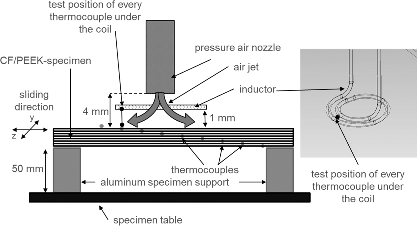
Setup for measuring temperature in thickness direction of laminates.

Figure 7.

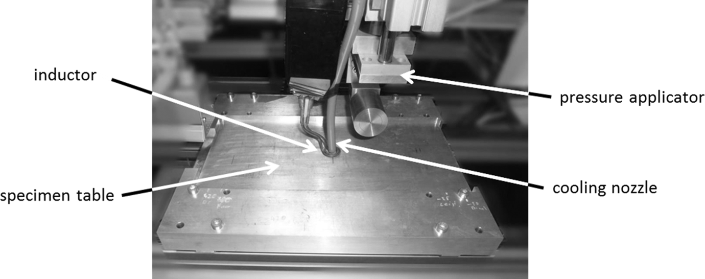
Inductive heating setup.

Modeling

For the calculation of the heat distribution in thickness direction, an analytical model is defined. The four dominating physical effects, such as inductive heating, heat conduction, thermal radiation, and thermal convection, are integrated in the model (see Figure 8). As an analytical model is applied, FEM software is not used. For simplification, only 1D-effects are considered. The thin thermocouple wires with a measuring area of approximately 0,008 mm² allow the assumption of a nearly homogeneous heat distribution in adjacent areas. Therefore, in-plane heat conduction is neglected and the heat flow is calculated in steps of 0.025 s to reduce overshoots. Every fifth output is compared with measured values. For a sufficient resolution in thickness direction, the temperature is calculated at each interface of the tapes and on both surfaces.

Figure 8.

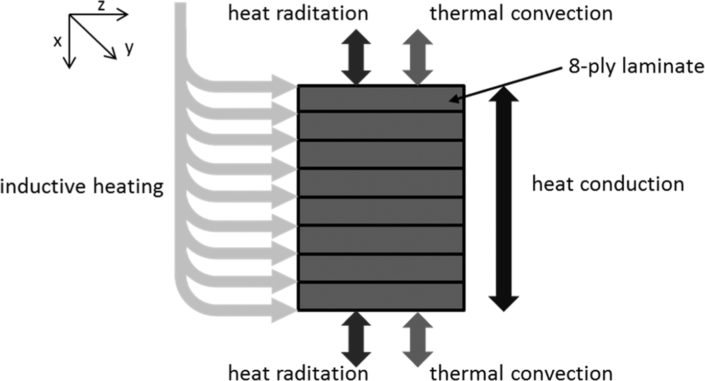
Schematic drawing of the model.

Inductive heating

The current density of the electromagnetic field in the laminate is mainly influenced by the distance to the coil and the thickness of the specimen. ⁷ As explained in “Experimental setup” section, the distribution of the current density in thickness direction changes if the specimen thickness is small in comparison with the skin depth (d < 10δ_s) The used specimen plates vary between 1.24 mm and 4.96 mm. Therefore, the equations (8) and (9) are used for calculating the induction heating energy input. However, Vrana ⁷ assumed that the entire electromagnetic field is reflected from the upper surface into the material. This assumption contradicts measurements presented in literature. Rudolf et al. ² , Moser, ³ and Miller et al. ⁸ did not research the through-thickness temperature distribution as a function of the laminate thickness and their results did not show a strong increase in the temperature by a reduction of the thickness. The research of Fink et al. ¹¹ also did not show a strong increase in the temperature. To connect the results presented in literature Vrana’s equation (9) is adapted by dividing it in two summands.

$\frac{e^{-\sqrt{2i}\frac{x}{{\delta }_S}}}{1\hspace{0.17em}-\hspace{0.17em}{e}^{-\sqrt{2i}\frac{2d}{{\delta }_S}}}$

18

$\frac{e^{\sqrt{2i}\frac{x}{{\delta }_S}}}{1\hspace{0.17em}-\hspace{0.17em}{e}^{\sqrt{2i}\frac{2d}{{\delta }_S}}}$

19

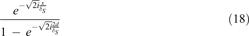
The first summand (equation (18)) describes the exponential decrease in the current density after entering into the material at the upper surface (towards the inductor). The second summand (equation (19)) describes the wave of the current density which is reflected at the lower surface. The denominator of both specifies the damping of the field due to the laminate/material properties (fiber volume ratio, void content, homogeneity, and so on). In contrast to other scientific induction heating models, ^11,28 only macroscopic effects are considered in the present model and the fitting coefficients K ₂ and K ₃ are implemented. These factors describe the laminate-dependent through-thickness decrease in the electromagnetic field. Furthermore, the factor K ₃ considers the temperature dependence of the electrical conductivity and, thus, the temperature dependence of the skin depth. Although Takahashi and Hahn and Nikolaos ^29,30 analytically describe the temperature dependence of the electrical conductivity for an epoxy composite material, the given thermal coefficients for this material cannot be used for the CF/PEEK material. To connect Vrana’s model with the results shown in literature, the surfaces of the laminate should neither be fully permeable nor reflect the complete electromagnetic field. Thus, the surfaces have to be semipermeable and a new coefficient K ₁ describes the laminate-dependent semipermeability of the laminate surfaces. The fitting factors are calculated iteratively by fitting the curve of the first researched laminate.

$j_z\left(x,t\right)\hspace{0.17em}=\hspace{0.17em}\frac{H_0}{K_3{\delta }_S}Re\left[\sqrt{2i}\left(\frac{e^{-\sqrt{2i}\frac{x}{K_3{\delta }_S}}}{1\hspace{0.17em}-\hspace{0.17em}{K}_2{e}^{-\sqrt{2i}\frac{2d}{K_3{d}_S}}}\hspace{0.17em}-\hspace{0.17em}\frac{K_1{e}^{\sqrt{2i}\frac{x}{K_3{\delta }_S}}}{1\hspace{0.17em}-\hspace{0.17em}{K}_2{e}^{\sqrt{2i}\frac{2d}{K_3{\delta }_S}}}\right)e^{i\omega t}\right]$

20

The skin depth δ_S is calculated with equation (17) and the material data (shown in Table 3). The magnetic field at the surface of the laminate H₀ is calculated according to Vrana ⁷ with I being the inductor current, x_it the distance between the two tubes of the inductor, x_i the distance between the inductor and the laminate, and r_i the radius of the inductor tube.

$H_0\hspace{0.17em}=\hspace{0.17em}\frac{I \text{* }\left(\frac{x_{it}}{2}\right)}{\pi \left({\left(\frac{x_{it}}{2}\right)}^2\hspace{0.17em}+\hspace{0.17em} {\left(x_i+ r_i\right)}^2\right)}$

21

Heat conduction

Despite the fact that induction welding is a highly nonuniform process, a steady state is assumed for each time step. This assumption is necessary for the implementation of the heat conduction into the analytical model. However, in order to reduce the effect of this assumption, the time steps for every steady state amounts to 0.025 s. Therefore, steady-state heat conduction can be implemented in the model ³¹ :

$\dot{Q}\hspace{0.17em}=\hspace{0.17em}-{\lambda }_{G}A\frac{\text{d}T}{\text{d}x}$

22

Heat radiation

With regard to heat radiation, a steady state is also assumed for each time step. According to Kabelac, ³¹ the radiation of the top (equation (23)) and lower (equation (24)) surface equations is implemented into the model. On the upper side, the radiation between the inductor, which was assumed as two cylinders, and the laminate is calculated to ${\dot{Q}}_{US}$ with the Stefan–Boltzmann constant σ_SB, the emissivity of the two bodies (laminate and inductor) ζ₁₁ and ζ₂₁, the considered areas A_W1 and A_W2, the distance between the inductor and the laminate’s surface x_I, the radius of the inductor tube r₁, and the temperature on the laminate’s upper surface T_o1 and at the inductor’s surface T_l1.

${\dot{Q}}_{US}=\frac{{\sigma }_{SB}{\zeta }_{11}{\zeta }_{21}{A}_{W1}\frac{1}{\pi }{\text{tan}}^{-1}\left(\frac{g}{x_I\hspace{0.17em}+\hspace{0.17em}{r}_1}\right)}{1\hspace{0.17em}-\hspace{0.17em}\left(1\hspace{0.17em}-\hspace{0.17em}{\zeta }_{11}\right)\left(1\hspace{0.17em}-\hspace{0.17em}{\zeta }_{21}\right){\left(\frac{1}{\pi }{\text{tan}}^{-1}\left(\frac{g}{x_I\hspace{0.17em}+\hspace{0.17em}{r}_1}\right)\right)}^2\frac{A_{w1}}{A_{w2}}}\left(T_{o1}^4\hspace{0.17em}-\hspace{0.17em}{T}_{l1}^4\right)$

23

On the lower side, the radiation between the laminate and the specimen table is calculated to ${\dot{Q}}_{\text{LS}}$ with the Stefan–Boltzmann constant σ_SB, the emissivity of the two bodies (laminate and specimen table) ζ₁₂ and ζ₂₂, the considered areas A_W1 and A_W2, the distance between the specimen table and the laminate’s surface x_d, the surface normals between the laminate and the specimen table β₁ and accordingly between the specimen table and the laminate β₂, and the temperature on the laminate’s lower surface T_o2 and at the specimen table T_l2.

${\dot{Q}}_{LS}=\frac{{\sigma }_{SB}{\zeta }_{12}{\zeta }_{22}{A}_{W1}\frac{1}{\pi }{\int }_{A_{w1}}^{ }{\int }_{A_{w2}}^{ }\frac{\text{cos}{\beta }_1\text{cos}{\beta }_2}{x_d^2}\text{d}{A}_{w2}\text{d}{A}_{w1}}{1\hspace{0.17em}-\hspace{0.17em}\left(1\hspace{0.17em}-\hspace{0.17em}{\zeta }_{12}\right)\left(1\hspace{0.17em}-\hspace{0.17em}{\zeta }_{22}\right){\left(\frac{1}{\pi }{\int }_{A_{w1}}^{ }{\int }_{A_{w2}}^{ }\frac{\text{cos}{\beta }_1\text{cos}{\beta }_2}{x_d^2}\text{d}{A}_{w2}\text{d}{A}_{w1}\right)}^2\frac{A_{w1}}{A_{w2}}}\left(T_{o2}^4\hspace{0.17em}-\hspace{0.17em}{T}_{l2}^4\right)$

24

Thermal convection

For thermal convection, a steady state is also assumed and implemented into the model

$\dot{Q}\hspace{0.17em}=\hspace{0.17em}\alpha A\text{d}T$

25

with

$\alpha \hspace{0.17em}=\hspace{0.17em}\frac{Nu {\lambda }_L}{L}$

26

Without air jet cooling on the lower and on the upper surface, natural convection is applied. ³¹ Due to the horizontal orientation of the laminate, two different Nusselt numbers have to be chosen for the upper and the lower surface. For the upper surface, the Nusselt number is ³¹

$Nu \hspace{0.17em}=\hspace{0.17em} 0.766{\left[Ra\hspace{0.17em}\cdot \hspace{0.17em}{\left[1\hspace{0.17em}+\hspace{0.17em}{\left(\frac{0.322}{Pr}\right)}^{\frac{11}{20}}\right]}^{-\frac{20}{11}}\right]}^{\frac{1}{5}}$

27

and for the lower surface, the Nusselt number is ³¹

$Nu\hspace{0.17em}=\hspace{0.17em}0.6{\left[Ra\hspace{0.17em}\cdot \hspace{0.17em}{\left[1\hspace{0.17em}+\hspace{0.17em}{\left(\frac{0.492}{Pr}\right)}^{\frac{9}{16}}\right]}^{-\frac{16}{9}}\right]}^{\frac{1}{5}}$

28

As a result of air jet cooling, natural convection on the upper surface is changed to forced convection with the Nusselt number ^31,32

$N{u}_l\hspace{0.17em}=\hspace{0.17em}\sqrt{N{u}_{l,\text{turb}}{ }^2\hspace{0.17em}+\hspace{0.17em}N{u}_{l,\text{lam}}{ }^2}$

29

in which

$N{u}_{l,\text{lam}}\hspace{0.17em}=\hspace{0.17em}0.332\sqrt{Re}\sqrt[3]{Pr}$

30

and

$N{u}_{l,\text{turb}}\hspace{0.17em}=\hspace{0.17em}\frac{0.0296R{e}^{0.8}Pr}{1\hspace{0.17em}+\hspace{0.17em}2.185R{e}^{-0.1}\left(Pr-1\right)}$

31

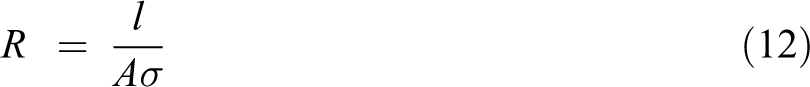
Results and discussion

Temperature distribution in thickness direction without air jet cooling

As a basis, the temperature distribution in thickness direction of the 16-ply laminate after 2 s of inductive heating is measured in order to calculate the three parameters (equation (20); K ₁, K ₂, and K ₃). In a second step, the temperature distributions in the 4- and 8-ply specimens are calculated and then measured for verification. In Figure 9, the temperature between the different layers for the three thicknesses is shown and the calculated values are compared with the measured ones. The temperatures are stated as percentages; in the following figures, 100% corresponds to the temperature (206°C) at the 8-ply specimen’s thermocouple position 1 without cooling the surface. The leading factor influencing the temperature distribution in thickness direction is the thickness of the specimen. A part of the electromagnetic field, which reaches the lower surface, is reflected in the laminate (described in equation (20)) and causes a temperature increase over the whole specimen thickness. The mirrored electromagnetic field intensity decreases with the specimen thickness because of the exponential decrease of the electromagnetic field in the specimen material. In comparison with the 4-ply laminate, the maximum temperature in the 16-ply laminate is 34% lower. Due to the increasing intensity of the mirrored electromagnetic field, the temperature distribution approaches the temperature distribution for infinite thick specimens (Figure 9) with an increasing thickness-skin depth ratio. This becomes apparent from a comparison between the temperature distributions of the 16-ply specimen and the infinite thick specimen (calculated). With this validated model, the temperature distribution in the laminate can be calculated for different specimen thicknesses. The constants (K₁, K₂, and δ_S) have to be recalculated when changing materials or layups. The difference between the temperature at 100% and the melting temperature of the laminate is greater than 100°C; therefore, the phase transformation does not have an impact on the temperature distribution. Yet, the theoretical model is applicable for higher temperatures after integrating the required material data.

Figure 9.

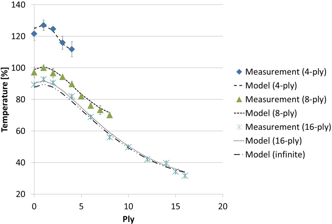
Through-thickness temperature distribution after 2 s and 10% power for varying specimen thicknesses.

Influence of the air jet flow rate

To prevent the top layers from melting while reaching the welding temperature in the interface, the surface has to be cooled. In Figure 10, the temperature distribution of the 8-ply laminate after 2 s of inductive heating with varying air jet volumes is shown. The highest temperature drop is measured at the surface. Here, the temperature falls from 97.1% of the reference temperature without cooling of the top surface to 73.9% of the reference temperature with 500 L min⁻¹ air jet cooling. Without cooling, the highest temperature is measured between the first and second plies. The temperature in this area decreases from 100% (with cooling) to 83.3% of the reference temperature without surface cooling. The temperature between the first and second plies drops below the temperature between the third and fourth plies in addition to the maximum temperature shifting to the interface of the second and third plies. A significant influence of the cooling can be measured up to the fourth ply. As a result, the temperature distribution can be optimized during the induction welding process when using cooling as a control of the hot spot should be possible with varying volumes. As shown in Figure 10, the model with cooling corresponds with the measured values.

Figure 10.

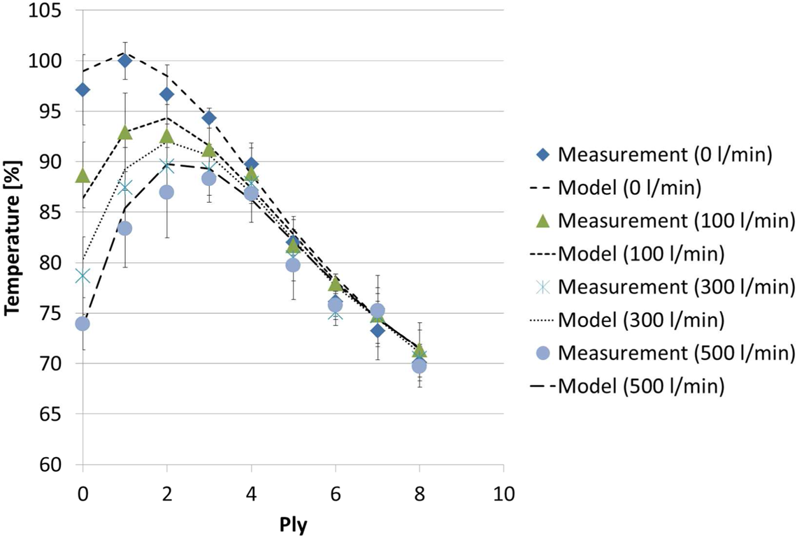
Through-thickness temperature distribution after 2 s and 10% power on 8-ply specimen with varying air jet volumes and 20°C air jet temperature.

Influence of the air jet volume temperature

Another influence on the temperature distribution while cooling with an air jet (100 L min⁻¹) is the temperature of the air jet itself. In Figure 11, the influence of the air jet volume temperature on the temperature distribution in thickness direction is shown. The cooling of the surface increases by 8.5 percentage points when the cooling temperature is reduced from 20°C to −30°C. A total input volume of 400 L min⁻¹ is necessary for a temperature reduction of the air jet to −30°C using the cyclone tube (cold air jet volume + hot air jet volume = total input volume). When comparing the temperature distribution of cooling with the cyclone tube (cold air jet: 100 L min⁻¹; temperature of the cold air jet: −30°C; hot air jet: 300 L min⁻¹; total input volume: 400 L min⁻¹) and without the cyclone effect (cold air jet: 400 L min⁻¹; temperature of the cold air jet: 25°C; hot air jet: 0 L min⁻¹; total input volume: 400 L min⁻¹), it leads to the result that within the measurement accuracy, both cooling types are equally effective (see Figure 12). A temperature difference of merely 1–2% points is measured between the first, second, and third plies. Yet, the technical effort of cooling with reduced temperature is higher. As a result, the temperature of the air jet is an additional parameter that allows to control the position of the hotspot and the use of cyclone tubes increases the efficiency of the process by consuming less pressurized air.

Figure 11.

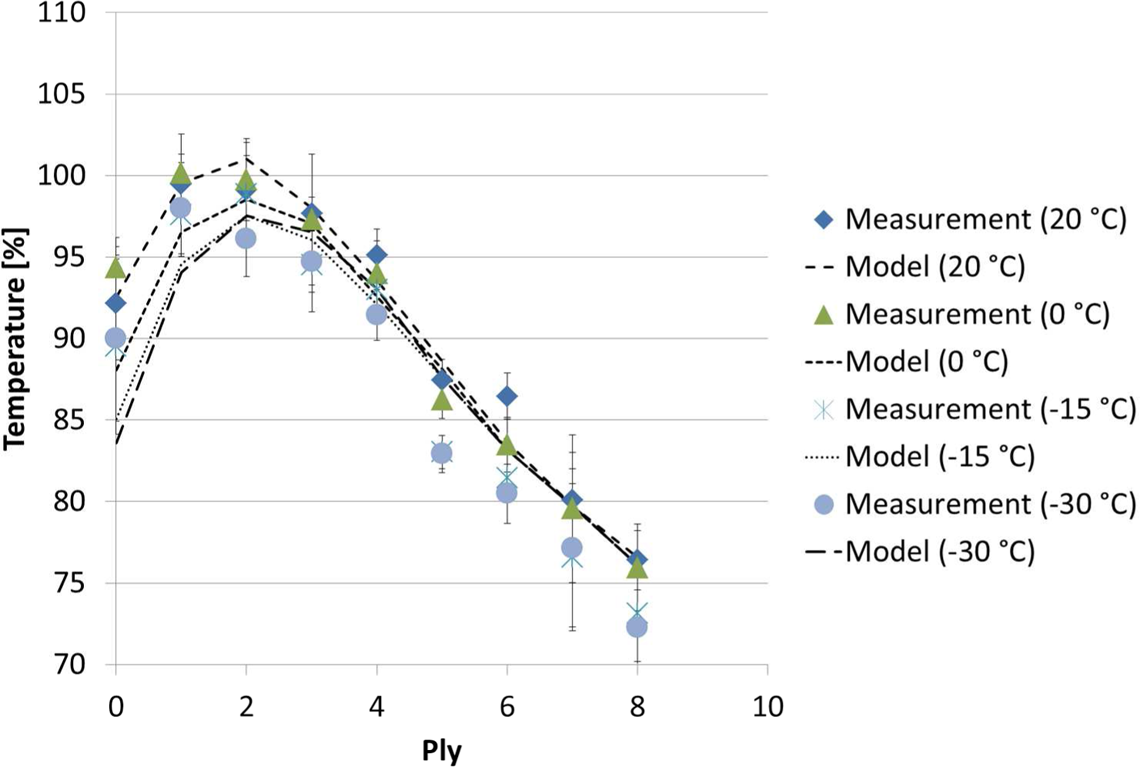
Through-thickness temperature distribution after 2 s and 10% power on 8-ply specimen with varying air jet temperatures and 100 L min⁻¹ cold air jet volume (total input volume (20°C): 100 L min⁻¹; total input volume (0°C): 320 L min⁻¹; total input volume (−15°C): 360 L min⁻¹; total input volume (−30°C): 400 L min⁻¹).

Figure 12.

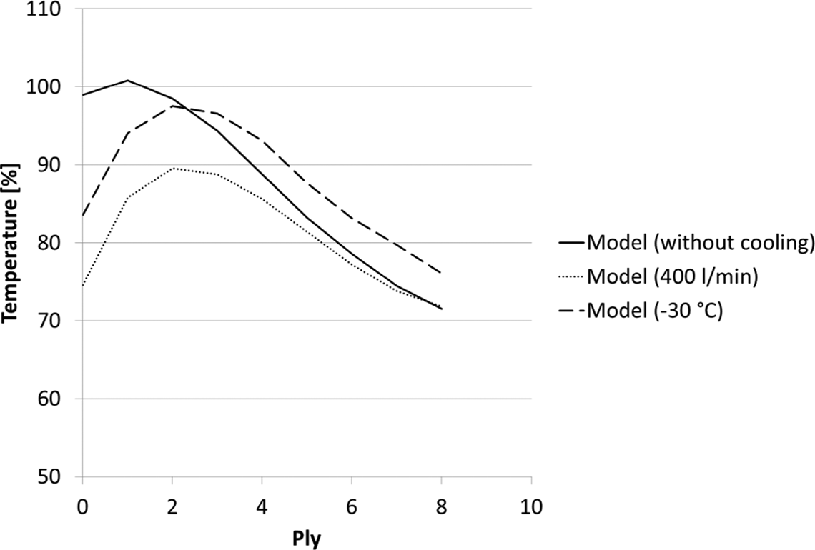
Through-thickness temperature distribution after 2 s and 10% power on 8-ply specimen with cyclone tube (cold air jet: 100 L min⁻¹; temperature of the cold air jet: −30°C; hot air jet: 300 L min⁻¹; total input volume: 400 L min⁻¹) and without cyclone effect (cold air jet: 400 L min⁻¹; temperature of the cold air jet: 25°C; hot air jet: 0 L min⁻¹; total input volume: 400 L min⁻¹).

Conclusion

This study presents a theoretical model to calculate the temperature distribution in thickness direction during the induction welding process. The model is validated by interlaminar temperature measurements. It is shown that the temperature is mainly influenced by the specimen thickness and the related skin depth ratio. By an increase in the ratio, meaning thicker laminates, the through-thickness temperature of the whole laminate decreases and converges to the temperature distribution for infinite thick specimens. Independent of the specimen thickness, the highest temperature in the laminate is reached between the first plies near the surface facing the inductor and not at the surface directly. This phenomenon can be explained by cooling by natural convection. When cooling the surface with an air jet, the maximum temperature can be shifted inwards. The temperature up to the interfaces of the second and third plies and of the third and fourth plies, respectively, has successfully been reduced by increasing the air jet volume up to 500 L min⁻¹. By a decrease of the temperature of the air jet, a further reduction in the temperature in the first plies is shown. In comparison with cooling with pressurized air by room temperature, cooling of the air jet using cyclone tubes (reduced air temperature) does not increase the efficiency of the process. With the presented method, a validated model for the calculation of the temperature distribution in thickness direction has been developed. Based on the model, the process for joining composites can be further developed.