Sage Journals: Discover world-class research

Abstract

Circadian rhythms are internal processes repeating approximately every 24 hours in living organisms. The dominant circadian pacemaker is synchronized to the environmental light-dark cycle. Other circadian pacemakers, which can have noncanonical circadian mechanisms, are revealed by arousing stimuli, such as scheduled feeding, palatable meals and running wheel access, or methamphetamine administration. Organisms also have ultradian rhythms, which have periods shorter than circadian rhythms. However, the biological mechanism, origin, and functional significance of ultradian rhythms are not well-elucidated. The dominant circadian rhythm often masks ultradian rhythms; therefore, we disabled the canonical circadian clock of mice by knocking out Per1/2/3 genes, where Per1 and Per2 are essential components of the mammalian light-sensitive circadian mechanism. Furthermore, we recorded wheel-running activity every minute under constant darkness for 272 days. We then investigated rhythmic components in the absence of external influences, applying unique multiscale time-resolved methods to analyze the oscillatory dynamics with time-varying frequencies. We found four rhythmic components with periods of ∼17 h, ∼8 h, ∼4 h, and ∼20 min. When the ∼17-h rhythm was prominent, the ∼8-h rhythm was of low amplitude. This phenomenon occurred periodically approximately every 2-3 weeks. We found that the ∼4-h and ∼20-min rhythms were harmonics of the ∼8-h rhythm. Coupling analysis of the ridge-extracted instantaneous frequencies revealed strong and stable phase coupling from the slower oscillations (∼17, ∼8, and ∼4 h) to the faster oscillations (∼20 min), and weak and less stable phase coupling in the reverse direction and between the slower oscillations. Together, this study elucidated the relationship between the oscillators in the absence of the canonical circadian clock, which is critical for understanding their functional significance. These studies are essential as disruption of circadian rhythms contributes to diseases, such as cancer and obesity, as well as mood disorders.

Keywords

circadian rhythms ultradian rhythms infradian rhythms biological oscillators time-varying oscillations multiscale oscillations phase dynamics nonlinear dynamics time-resolved analysis

Humans, like all living organisms, are subject to internal biological rhythms which are molded by external forces. Our bodies are attuned to the environment; our behavioral and physiological outputs are shaped by geophysical cycles. Earth is our home, and every step of our evolution from single cells to complex organisms has polished our capability to survive under the conditions dictated by this environment. By organizing our behavior and physiology with respect to the outside world, we are energy-efficient machines.

Biological rhythms are outputs of interacting, thermodynamically open systems which are exposed to continuous external influences. Mathematically, these systems are nonautonomous, nonlinear, and predominantly deterministic. Nonautonomous systems are dynamical systems that are explicitly time-dependent (Kloeden and Rasmussen, 2011). This means that their frequencies, phases, and couplings can be all functions of time. Physically, they are not independent of the environment, so external perturbations need to be taken explicitly into account. They are largely deterministic; however, when time is not considered, that is, when they are represented in the phase space or the frequency domain, their properties are often misinterpreted as stochastic (Clemson and Stefanovska, 2014). Their resultant dynamics are time-varying, so nonautonomous clocks are not perfect. They have adjustable frequencies, and time is a physical quantity; hence, their dynamics are not the same when time is reversed (Stefanovska and McClintock, 2021; Kloeden and Yang, 2020; Suprunenko et al., 2013). They need to be treated with finite-time methods, both in modeling approaches and in the methods with which their time series are analyzed (Newman et al., 2021). In what follows, we will use finite-time methods throughout.

The most well known biological rhythm is the circadian rhythm; the approximately 24-h cycle of physiology and behavior which is synchronized to the environmental light-dark cycle (Dibner et al., 2010; Morse and Sassone-Corsi, 2002), and characterizes most living organisms. A thorough investigation into the timekeeping mechanism is highly essential, as disruption of circadian rhythms contributes to the onset of diseases such as cancer and obesity (Barger et al., 2009) as well as mood disorders such as depression (McClung, 2007).

The circadian system is governed by self-sustaining circadian clocks that exist in most cells (Dunlap, 1999; Shearman, Sriram et al., 2000; Brown et al., 2019). Coupling occurs between the clocks, forming a network of interacting biological oscillators. The clock components are clock genes and proteins, and the clock mechanism is composed of transcription-translation feedback loops (Hastings et al., 2018). Positive regulators (CLOCK and BMAL1) drive the transcription of negative regulators (PER and CRY). PER-CRY complexes accumulate during the circadian day, which inhibits the positive regulators and so acts negatively on their own transcription. During the circadian night, the PER-CRY complexes degrade and their transcription levels fall, and the cycle begins again. Further accessory loops stabilize the transcription levels of the positive regulators. This mechanism then leads to ∼24-h oscillations of clock gene transcript and protein levels which are responsible for the organism’s 24-h body clock.

The circadian rhythm is entrained to the 24-h environmental light-dark cycle. In mammals, a primary circadian pacemaker exists in the suprachiasmatic nucleus (SCN), a small region of the brain (Weaver, 1998). The SCN is responsible for coordinating the phase of circadian clocks throughout the mammal. The SCN obtains information about the time of day through light (Morse and Sassone-Corsi, 2002; LeGates et al., 2014; Foster et al., 2020), due to the circadian clocks within the SCN being light-entrainable oscillators (LEOs). Light enters the system via the eyes and is then transmitted to the SCN. The SCN then coordinates the phase of the rest of the body clocks. Living organisms then adapt and organize their physiology and behavior according to the time of day.

Light is the dominant environmental information that is responsible for entraining the circadian rhythm. However, other circadian pacemakers exist which respond to other stimuli. In rodents, researchers have discovered the following oscillators: the food-entrainable oscillator (FEO), the methamphetamine sensitive circadian oscillator (MASCO), the palatable meal-inducible circadian oscillator (PICO) and the wheel inducible circadian oscillator (WICO) (Pendergast and Yamazaki, 2017). The locations of these oscillators are unknown, but the MASCO and FEO are known to exist outside the SCN. Therefore, scheduled feeding, methamphetamine treatment, palatable meals and wheel access also give timing cues, and behavioral rhythms exhibit the outputs of these extra-SCN oscillators. In rodents with SCN-lesions or disabled canonical circadian transcriptional-translational feedback clock mechanisms, outputs are still seen from the other circadian pacemakers (Mohawk et al., 2009; Storch and Weitz, 2009; Pendergast and Yamazaki, 2017). Therefore, they have a different molecular timekeeping mechanism than the LEO. The FEO, MASCO, PICO and WICO run with the same period (Pendergast et al., 2012; Flores et al., 2016), and the corresponding stimuli increase dopamine tone (Pendergast and Yamazaki, 2017). Therefore, these secondary pacemakers entrain to arousing stimuli. The LEO and these secondary oscillators are speculated to be coupled (Pendergast and Yamazaki, 2017), forming a circadian timing system complex. The timing cues all influence the phase and period of circadian clocks throughout the body.

Biological rhythms with periods substantially shorter than 24 h have been detected (Goh et al., 2019); such rhythms are termed ultradian rhythms. Ultradian frequencies of many physiological processes have been detected in most living systems, from single cells (Kippert and Hunt, 2000) to more complex organisms. However, their biological mechanism, origin and functional significance are yet to be understood. It is also unknown whether there is a universal ultradian mechanism, or if there are multiple.

Ultradian rhythms exist in the presence (Dowse et al., 2010) and absence (Gerkema et al., 1990) of the circadian cycle, which highlights their importance. Sufficient evidence has been provided that ultradian rhythms are independent of the LEO in the SCN, suggesting a separate mechanism and origin (Gerkema et al., 1990; Stephenson et al., 2012; Waite et al., 2012). Ultradian rhythms do not correspond to any known geophysical cycles. Early work by Bash (1939) showed that an ultradian hunger drive persists in the absence of neural impulses from the stomach; suggesting this internal clock continues ticking regardless of the state of the system. Ultradian rhythms in mammals have been hypothesized to be of cellular origin, with a network in place to synchronize and coordinate the rhythms (Wu et al., 2018).

The purpose of this article is to investigate the behavioral rhythms that remain in a biological system after the canonical circadian timekeeping mechanism is disabled and in the absence of external stimuli. Biological systems cannot be modeled easily, and through approximations, the most exciting characteristics are lost. Oscillators within biological systems may have time-varying frequencies, phases, amplitudes and interactions. Therefore, novel numerical methods must be applied to decipher their complex dynamics. The time series obtained by monitoring behavior over time have been analyzed using unique set of methods that enable multioscillatory dynamics to be time-resolved (Clemson and Stefanovska, 2014; Clemson et al., 2016), available as the MatLab/Python toolbox MODA (Newman et al., 2018). The algorithms utilize the phases and amplitudes from the signals, rather than only amplitudes which are more prone to noise and artifacts, and do not assume that phases/frequencies are constant. The data under analysis are particularly long for this line of research (272 days) and were sampled frequently (every 1 min), suitable to observe patterns that emerge over time and rhythms that repeat on scales from days to minutes.

Rhythms do not have strict frequencies, but vary around certain values; therefore, it is of utmost importance to investigate their time-variable dynamical properties which are often ignored. We first determine the oscillatory components and their dependence on time using the wavelet transform (Daubechies, 1992; Kaiser, 1994; Iatsenko et al., 2015). Then, we investigated whether any of the oscillatory components exist in harmonic relationships (Sheppard et al., 2011) to determine the number of basic oscillators within the system in a given time-frame. The instantaneous frequencies of the oscillatory components are then extracted using ridge curve extraction (Delprat et al., 1992; Carmona et al., 1997, 1999; Iatsenko et al., 2016) before determining their interactions and couplings (Jensen and Colgin, 2007; Stankovski et al., 2019) using dynamical Bayesian inference (DBI) (Smelyanskiy et al., 2005; Stankovski et al., 2012, 2014). Wavelet phase coherence (Le Van Quyen et al., 2001; Lachaux et al., 2002; Bandrivskyy et al., 2004; Grinsted et al., 2004; Sheppard et al., 2012) is used to investigate whether the system is fully autonomous or whether some of the observed oscillations are responsive to some external perturbation. An origin for the observed oscillations is suggested based on the results obtained with such analyses, as well as using current understanding from existing studies. The overarching aim is to understand which rhythms remain after the dominant canonical circadian system is disabled.

Materials and Methods

Biological System

To determine whether a timekeeping mechanism other than the circadian rhythm exists, the circadian system must be disabled in the organism under investigation. When investigating rodents, either SCN-lesioned or knockout mice are used. Knockout mice are genetically modified mice, where the function of a gene has been inactivated or “knocked out”. In this case, it is the circadian clock genes that must be knocked out, such as the Period genes (Per1, Per2, and Per3). Knocking out clock genes disrupts the clock mechanism generating the circadian rhythm.

Single knockout Per1^−/−, Per2^−/−, and Per3^−/− mice (in congenic with 129/Sv genetic background provided by David Weaver, University of Massachusetts Medical School, Worcester, MA, USA) (Shearman et al., 2000; Bae et al., 2001) were backcrossed with C57BL/6J mice (Jackson Laboratory #000664) for 15 generations. The Per mutant mice were then crossed until Per1^+/−; Per2^−/−; Per3^−/− mice were generated. The Per1^+/−; Per2^−/−; Per3^−/− mice were maintained by intercross at Vanderbilt University (Pendergast et al., 2009, 2010) and then UT Southwestern Medical Center (Flores et al., 2016). The Nr1d1–luciferase reporter mouse line, in which the Nrd1d1 (also known as Rev–erb) promoter drives the expression of luciferase, was generated in a C57BL/6NCrL background (Charles River #027). 3.8 kb mNrd1d1 promoter was cloned into Mlu I/Nco I site of the pGL3 BASIC firefly luciferase reporter vector (Promega, Madison, WI, USA). Transgenic mice were generated at the Southwestern Transgenic Technology core using a 7.6 kb mNrd1d1-luc reporter construct linearized by Dra III and Ase I. Transgenic mice were identified by using PCR to detect a 195 bp fragment from tail DNA (forward primer, 5’– accctccccttgtgttctct –3’; reverse primer, 5’– tccacctcgatatgtgcatc –3’). Among the nine founders that had luciferase activity, we established two Nrd1d1-luc transgenic lines. Line #60 was crossed with C57BL/6J mice obtained from the UT Southwestern Wakeland Mouse Breeding core for 1 generation. Per1^+/−; Per2^−/−; Per3^−/− mice (F7) were crossed with hemizygous Nr1d1-luciferase (N1) mice. The offspring were intercrossed for 2–4 generations to generate experimental mice. Those mice were generated for the project identifying putative locations of the methamphetamine-sensitive circadian oscillator; and the luciferase reporter was not used in the current study.

All mice were bred and group-housed in a 12L:12D cycle. Five Per1^−/−; Per2^−/−; Per3^−/− mice (one female) with hemizygous Nr1d1-luciferase transgene, aged 4-5 months old were used for this study. Circadian behavior recordings were conducted in a light-tight ventilated box (Phenome Technologies, Skokie, IL, USA). The mice were singly housed in plastic cages (length × width × height: 29.5 × 11.5 × 12.0 cm) with running wheels (diameter: 11 cm) in constant darkness with ad libitum access to regular chow (2018 Teklad Global 18% Protein Rodent Diet; Harlan, Madison, WI, USA) and water throughout behavior recordings for 272 days. Wheel revolutions were continuously recorded every minute (ClockLab system ver. 3.604; Actimetrics, Wilmette, IL, USA). Temperature and relative humidity inside of the light-tight box were recorded every 5 min ( $22.4 \pm 0.4 ° C$ , min $= 21.3 \circ C$ , max $= 24.6 \circ C$ ; $44.5 \pm 7.1 %$ , min $= 15.2 %$ , max $= 60 %$ ) by Chamber Controller software (ver. 4.104; Actimetrics). Their dynamical characteristics are shown in the Supplementary Material. Cages and water bottles were changed in the dark by a researcher wearing an infrared viewer (FIND-R-SCOPE Infrared Viewer; FJW Optical Systems, Inc. Palatine, IL, USA) without exposing mice to visible light. All mice were in the same light-tight box and treated the same way. Times when cage changes and visual inspections were conducted were recorded. All animal experiments were conducted in accordance with the guidelines of the Institutional Animal Care and Use Committee at UT Southwestern Medical Center (protocol #2016-101376). Male and female actogram examples are shown in Figure 1.

Figure 1.

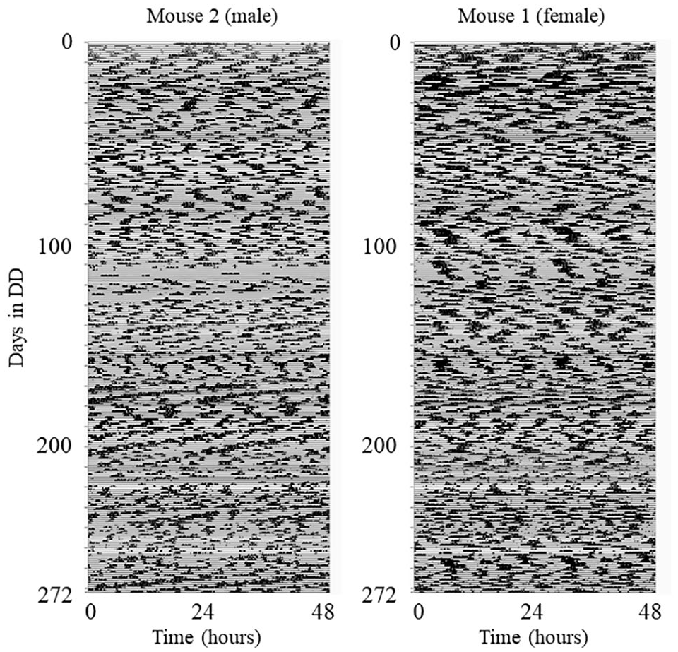
Wheel-running activity of Per1^−/−; Per2^−/−; Per3^−/− mice. Wheel revolutions were collected in 1-min bins and were binned with 10 min and plotted with ClockLab (percentile plot). An example of each sex is shown. There are missing data for mouse 2 for ∼60 h between days 113 and 118 due to a micro-switch problem.

Due to a micro-switch problem, there are missing data for mouse 2 for ∼60 h between days 113 and 118 (Figure 1, left). In addition, for a small number of data points ( $0.09 %$ ), due to rebooting the PC or a ClockLab software problem, the PC recorded no value; this occurred at the same time for all mice. The most prolonged period this occurred for was 2 h, which over 272 days can be considered as negligible. All missing data points were assigned a value of 0, so the time series could later be used as an input in the analyses that all require equidistantly spaced data with a numerical value. Due to the very low percentage of missing data points, no effect on the overall results is expected.

Preprocessing

Before performing analysis on the biological system, the signal must be preprocessed (Iatsenko et al., 2015; Newman et al., 2018). The signal is first detrended, which includes removing nonoscillatory trends from the original signal by subtracting a best-fit cubic polynomial. Nonoscillatory trends are represented as low-frequency oscillations, and detrending removes the effects of their possible interference with low-frequency oscillatory components of interest. The frequencies of interest are then determined, and the time series is filtered of frequencies outside the frequency interval of interest, by nullifying their amplitudes. The preprocessing, as well as all time series analysis methods explained below, were applied to the original data sampled at intervals of 1 min.

Time-Frequency Analysis

For the nonautonomous system under investigation, representation in the frequency domain is insufficient in obtaining all the information contained within the signals. Traditionally, time-dependence is treated as noise and frequencies are time-averaged. In this study, the time series are transformed to the time-frequency domain via the wavelet transform, to extract the oscillatory components over time.

The wavelet of choice is the lognormal wavelet, which has better resolution than the well-known Morlet wavelet (Iatsenko et al., 2015), as the amplitude and power are symmetric around the peak. The wavelet slides over the signal, and the section of the signal overlapping with the wavelet is transformed to the frequency domain. The scale of the wavelet is adjusted depending on the frequency to be obtained, to optimize the frequency resolution and time-localization trade-off. The wavelet scale is inversely proportional to time localization and directly proportional to frequency resolution. Therefore, smaller scales are used to observe higher frequencies and larger scales are used to observe lower frequencies. The frequency resolution parameter determines the trade-off between time localization and frequency resolution; the higher the value, the higher the frequency resolution and the lower the time resolution. In this study, the frequency resolution parameter value that provided an optimal trade-off was 1.8. Wavelet power plots are produced by squaring the absolute value of the wavelet amplitudes, then time-averaged.

Initial time-frequency analysis was performed over all possible frequencies. The time between sample points is 1 min, and the highest frequency that can be resolved is twice this time, 2 min (Nyquist theorem). A lower frequency limit of ∼28 days was determined by the length of the recording (272 days) and the frequency resolution (1.8). The lower frequency limit was refined by identifying the lowest significant frequency that was detected across all mice, so frequencies below $0.00055 \min^{- 1}$ (∼30.3 h) are filtered out.

The cone of influence is the area in the time-frequency domain that corresponds to half of the window length used for each of the estimated frequencies—both at the beginning and the end of a recorded signal. Because of the logarithmic frequency resolution, it has an exponential shape. To overcome this, when ridge extraction is performed, zero-padding is added to the start and the end of the signal, so that ridges are extracted for the entire time of recording (Iatsenko et al., 2016).

Ridge Curve Extraction

Ridge curve extraction is a method to extract the trace of a time-varying frequency from a time-frequency representation of a signal (Delprat et al., 1992; Carmona et al., 1997, 1999; Iatsenko et al., 2016). The time-varying frequencies are seen as amplitude peaks in the time-frequency representation and are referred to as ridge curves. Oscillatory components with their corresponding frequencies are identified visually by using both the time-frequency representation and the time-averaged power plot (see Figures 2a and 2b).

Figure 2.

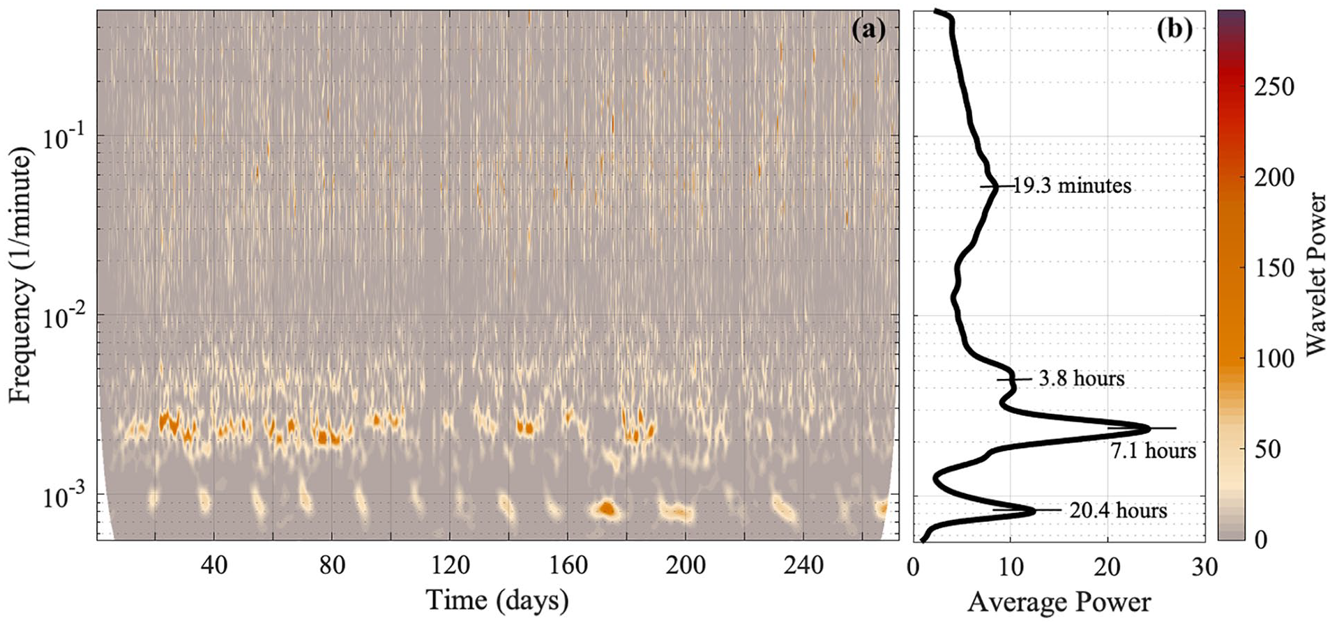
(a) The time-frequency representation (obtained via the wavelet transform) of behavioral data from mouse 2, where the “Wavelet power” is the squared amplitude of the wavelet, and (b) the corresponding time-averaged power spectrum. The y-axis is presented on a logarithmic scale. Four oscillatory components emerge. The wavelet power and the average power have units (wheel revolutions/min)². TFR = time-frequency representation.

For ridge extraction, a frequency band must be defined which includes the entirety of the oscillatory component. The frequency band should include the whole width of the oscillatory component, including the peak and the interval in which the frequency variability manifests. Caution was necessary when extracting the oscillatory components, as some are very close together and partially adjoined. For accurate results, only one oscillatory component should exist in the frequency band. The frequency bands for each oscillatory component were chosen based on the time-frequency representation and the average power spectrum. Minima in the average power spectrum were used as starting boundaries, which then based on the time-frequency representation were corrected to avoid overlapping of oscillatory components. For each mouse, the frequency bands of different oscillatory components did not overlap. Figure 3 gives an example of the chosen boundaries for ridge extraction, and the ridges for each oscillation in each mouse are shown in the Supplementary Material. Ridge curves are given by the time sequence of maximum amplitude peaks in time-frequency space within the frequency interval specified.

Figure 3.

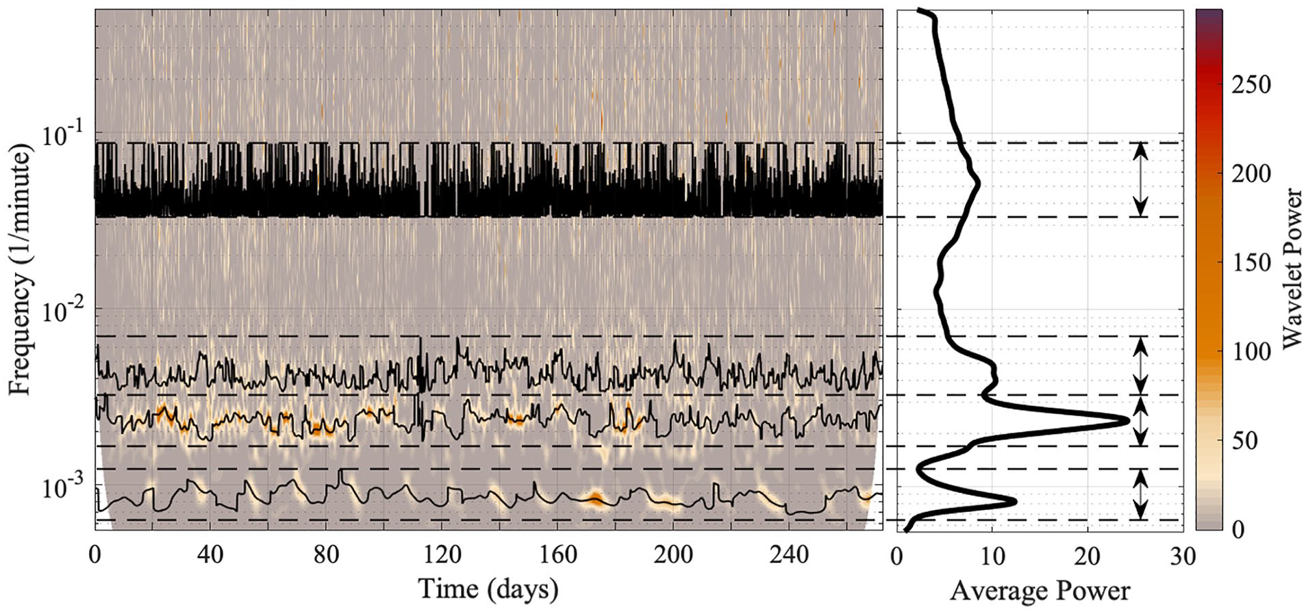
The method for extracting ridges from a time-frequency representation, and the extracted ridges. The wavelet transform is performed on the behavioral data of mouse 2. For ridge extraction, the chosen boundaries must contain the entirety of, and only, the oscillatory component under investigation, and are shown by the dashed lines and two-way arrows. Both the time-frequency representation and the average power spectrum are used to determine the correct boundaries. The wavelet power and the average power have units (wheel revolutions/min)². TFR = time-frequency representation.

Violin plots (Hoffmann, 2015) were created for each oscillation using the frequency data extracted from ridge analysis for all mice, to visualize the spread of the data.

Harmonic Finder

The oscillatory components extracted from the time-frequency representation may be in harmonic relationships: the instantaneous frequencies of an oscillation are multiples of the instantaneous frequencies of another at all times. Harmonics arise due to a single oscillator having a nonsinusoidal wave shape, which then in the frequency domain is represented with additional oscillatory components, at multiple frequencies of the basic frequency. Investigating harmonic relationships is essential to determine the number of basic oscillators, or modes, that characterize the biological system. By establishing the distinct oscillators, the fundamental origin of their rhythms can then be investigated.

A preliminary, visual harmonic test can be performed by comparing the extracted ridges; if the frequencies are in a harmonic relation, their ridges should have similar shapes. Then, the possibility of a harmonic relationship may be investigated by determining whether the oscillatory components consistently exist in a rational relationship over time. However, a more reliable method has been developed by Sheppard et al. (2011), specially designed to find a harmonic relationship between oscillatory components with time-varying frequencies and amplitudes, using wavelets.

The phase time series of each frequency component are extracted using the wavelet transform, and are compared pairwise. The algorithm calculates the mutual information between the pair to determine whether a harmonic relationship exists. The frequency interval of interest is from $6 \times 10^{- 4} \min^{- 1}$ (corresponding to a period of ∼27.8 h) to $0.5 \min^{- 1}$ (a period of 2 min), which includes the entirety of the oscillatory components of interest, determined after time-frequency analysis.

For the wavelet transform, a time resolution of $360 \min$ is used (which is the length of the wavelet), as it gave the optimal trade-off between time and frequency resolution. The method of surrogates is used to test the statistical significance. For computational reasons, a minimum of 19 amplitude-adjusted Fourier transform (AAFT) surrogates were used, which has been demonstrated to be the acceptable minimum (Lancaster et al., 2018). The harmonic results are shown relative to the mean and standard deviation of the surrogate distribution.

Dynamical Bayesian Inference

Dynamical Bayesian Inference (DBI) (Smelyanskiy et al., 2005; Stankovski et al., 2012, 2014) is a method to determine whether a pair of oscillators within a system are coupled, and if so, how they are coupled. Phase coupling is determined by how an oscillator influences the phase of another oscillator. Within a biological system, the frequencies and amplitudes of oscillators may be time-varying; therefore, their interactions may also evolve in time. Within a time window that is slid along a signal, DBI determines the time evolution of couplings between oscillators. Therefore, it is chosen over techniques that determine time-independent coupling (Rosenblum and Pikovsky, 2001; Paluš and Stefanovska, 2003) to understand the true underlying nature of the system. DBI is based on Bayes’ theorem: prior knowledge of the evolution of the system is used to help determine its current condition. It uses a customized information propagation procedure within the Bayesian framework, which allows for time-evolving dynamics to be inferred (Smelyanskiy et al., 2005; Stankovski et al., 2012, 2017).

The interactions between all combinations of phases of pairs of oscillators for the same animal are investigated. The instantaneous frequencies of an individual oscillatory component are obtained from the time-frequency representsation using ridge extraction. For accurate results, during ridge extraction, the oscillatory components must occupy disjoint frequency bands to exclude interference.

Time-independent coupling strength approximations are computed within specified time windows. For each time window, the strength of the coupling is calculated by determining whether the phase of one oscillator is influenced by the other and vice versa. The window size must be at least 10 cycles of the lowest frequency across the two frequency bands being investigated for coupling. For consistency, this lowest frequency is determined across all the mice. Therefore, the width of the time windows are chosen to be $15, 880$ min, and time windows overlap by $75 %$ .

The Fourier order, $K > 0$ , determines the number of degrees of freedom, ${(2 K + 1)}^{2}$ , for each coupling when determining the interaction between two oscillators (Newman et al., 2018). A Fourier order of 2 was empirically determined, which gives a sufficient number of degrees of freedom (25 for each coupling) without introducing too many which causes overfitting leading to highly inaccurate predictions.

After obtaining results for a time window, the amount that these results affect the calculation for the subsequent window is determined by the propagation constant $p \geq 0$ . The larger the value of $p$ , the less the results are incorporated into the algorithm for the next window. A value of $0.2$ was used; however, after investigation, using different values did not change the end coupling strength results.

Surrogates are used to test the statistical significance of the coupling between two oscillators. As there is for sure no coupling between the surrogates and the oscillators under investigation, the method of surrogates gives a relative value of the coupling strength. For computational reasons, a minimum of 19 cyclic phase permutation (CPP) surrogates are used, which has been demonstrated to be the acceptable minimum (Lancaster et al., 2018), and the test is performed with a significance level of $= 0.05$ .

Wavelet Phase Coherence

Wavelet phase coherence (Le Van Quyen et al., 2001; Lachaux et al., 2002; Bandrivskyy et al., 2004; Grinsted et al., 2004; Sheppard et al., 2012) investigates the relationship between phases from two time series over time, at each frequency of interest. If the coherence is high, then the two sources are either mutually coupled, or they have a common external driver that influences their dynamics. Phase coherence is investigated for all the possible pairs of signals.

The wavelet transform is performed for the pair of signals under investigation. During the wavelet transform of the two signals, instantaneous phases are assigned to the oscillatory processes at frequency f over time. The instantaneous phase coherence is a measure of how close the instantaneous phase difference is to being constant between the oscillatory processes at frequency f with an output between 0 (no coherence) and 1 (perfect coherence). The average phase coherence at frequency f is then calculated. For high values of phase coherence, an external driver with frequency f may be influencing both signals, or they have mutually coupled oscillations.

The higher and lower frequency limits were refined by identifying the highest and lowest significant frequencies that were detected across all mice, and so wavelet phase coherence is investigated for frequencies between 0.007 min⁻¹ (∼2.4 h) and 0.00004 min⁻¹ (∼17.4 days).

Phase coherence values are often nonzero for oscillations that are completely unrelated; therefore, the significance of the results must be tested. A surrogate-based significance test is used to determine the significance of the results using 30 AAFT surrogates. The test is performed with a significance level $α = 1 / (30 + 1)$ .

The median absolute coherence was then calculated to see what is common among all the mice. For each mouse pair, the absolute coherence was calculated by subtracting the surrogate data. Then, the median was calculated at each frequency, along with the 90th percentile to show the spread of the data.

Surrogates

Surrogates are signals used to determine whether a system has a certain property; they behave like the system but do not possess the property under investigation (Lancaster et al., 2018). The surrogates and the original data are treated in the same way, so any process applied to the original data is also applied to the surrogates.

For this study, surrogates are used to test the significance of results obtained during DBI, the analysis for the possible existence of high harmonic components using the harmonic finder algorithm, and in the analysis of wavelet phase coherence. The surrogates are created from the signals. DBI uses CPP surrogates. The signals used in DBI are phase signals, that is, they cycle from 0 to 2π over time. The signal is divided into complete cycles, which are then randomly permuted. The cycles at the beginning and end, which are not complete, stay fixed. In the analysis for the possible existence of high harmonics as well as wavelet phase coherence analysis, AAFT surrogates are used. A Gaussian noise signal $G$ is generated, and its values and the values of the original signal $S$ are ranked from smallest to largest. $G$ is then reordered to match the rank order of $S$ , to create signal $X$ . $X$ is Fourier transformed, creating $X_{F T}$ , and the values of $X_{F T}$ are ranked from smallest to largest. The original signal $S$ is then reordered to match the rank order of $X_{F T}$ to give the surrogates.

The appropriate analysis technique is applied to the original data and the surrogate set. The result given by the original system is compared with the distribution of the results given by the surrogates. If the comparison shows a significant difference, one can propose that the original data, and hence the system they represent, possess a particular property with a certain confidence level. Otherwise, the system cannot be considered to have such a property, or the test is too inadequate to prove this.

Results

Oscillatory Components

By performing the wavelet transform on the signals, it was discovered that Per1/2/3 triple knockout mice in constant darkness had wheel-running rhythms that were less than 24 h. A similar time-frequency representation was obtained for all mice, and an example is shown in Figure 2a (time-frequency representations for all five mice data are shown in the Supplementary Material, Figures S1-S3). In the average power plots, with an example shown in Figure 2b, two narrow peaks reside in the longer period end (oscillation 1 and oscillation 2; see Tables 1 and 2). Oscillation 2 always has more extensive power than oscillation 1. A less distinct peak with a shorter period is located near oscillation 2 (oscillation 3; see Tables 1 and 2). A broader peak exists in the shorter period end (oscillation 4; see Tables 1 and 2).

Table 1.

The oscillatory components within the murine behavioral data.

Oscillation	Mouse 1	Mouse 2	Mouse 3	Mouse 4	Mouse 5
1	15.5 h	20.4 h	15.9 h	17.9 h	16.5 h
2	8.3 h	7.1 h	6.0 h	8.9 h	8.5 h
3	4.8 h	3.8 h	3.5 h	4.7 h	3.3 h
4	22.2 min	19.3 min	19.8 min	16.0 min	17.0 min

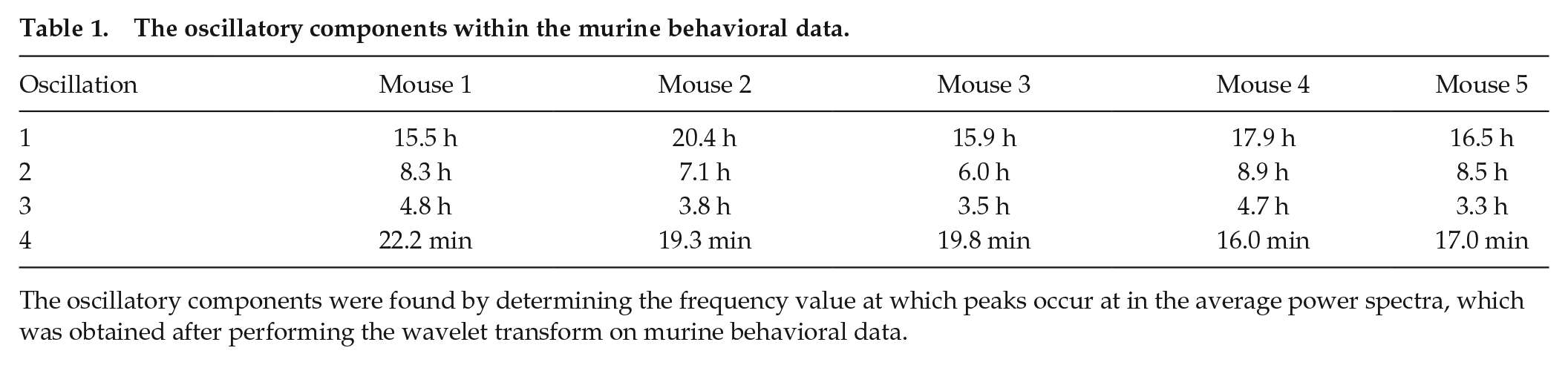
The oscillatory components were found by determining the frequency value at which peaks occur at in the average power spectra, which was obtained after performing the wavelet transform on murine behavioral data.

Table 2.

The oscillatory components within the murine behavioral data.

Oscillation	Mouse 1	Mouse 2	Mouse 3	Mouse 4	Mouse 5
1	14.9 ± 2.1 h	19.9 ± 2.0 h	15.8 ± 2.2 h	17.7 ± 2.3 h	16.7 ± 1.8 h
2	8.4 ± 1.0 h	7.3 ± 0.8 h	5.6 ± 0.8 h	8.9 ± 1.1 h	8.4 ± 1.2 h
3	4.2 ± 0.4 h	4.0 ± 0.5 h	3.1 ± 0.4 h	4.7 ± 0.5 h	3.9 ± 0.5 h
4	24.5 ± 4.2 min	25.3 ± 4.1 min	25.4 ± 3.9 min	25.2 ± 4.2 min	24.6 ± 3.9 min

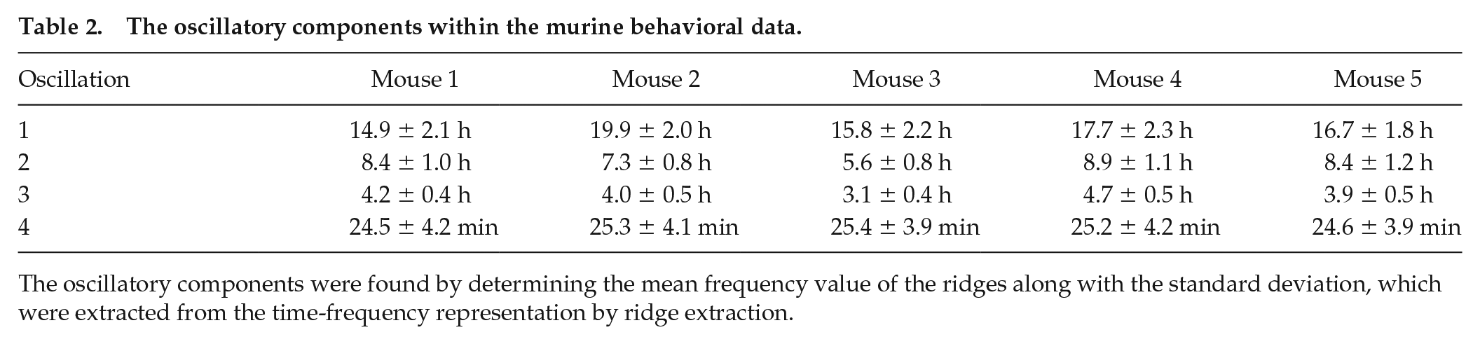
The oscillatory components were found by determining the mean frequency value of the ridges along with the standard deviation, which were extracted from the time-frequency representation by ridge extraction.

Violin plots for periods of each oscillation are shown in Figure 4 to visualize the spread of the data. The frequency peaks of the oscillatory components are given in Tables 1 and 2. The values in Table 1 were found by determining the frequency value at which peaks occur at in the average power spectra. The values in Table 2 were found by determining the average frequency value of the ridges, which were extracted from the time-frequency representation by ridge extraction. The mean period of oscillation 4 listed in Table 2 may be slightly lower than actuality because the frequency resolution parameter of 1.8 for the wavelet transform, based on which the ridges were detected, is least optimal for the upper end of the frequency interval investigated. This interval spans the range from 0.00055 min−1 (30.3 h) to 0.5 min−1 (2 min). It is difficult to preserve the same optimal compromise between time localization and frequency resolution over such a large interval, due to the Heisenberg uncertainty principle. Yet, for the sake of comparison, a single resolution frequency was used, rather than dividing the frequency interval into two parts and calculating the frequency content with two different resolution frequencies.

Figure 4.

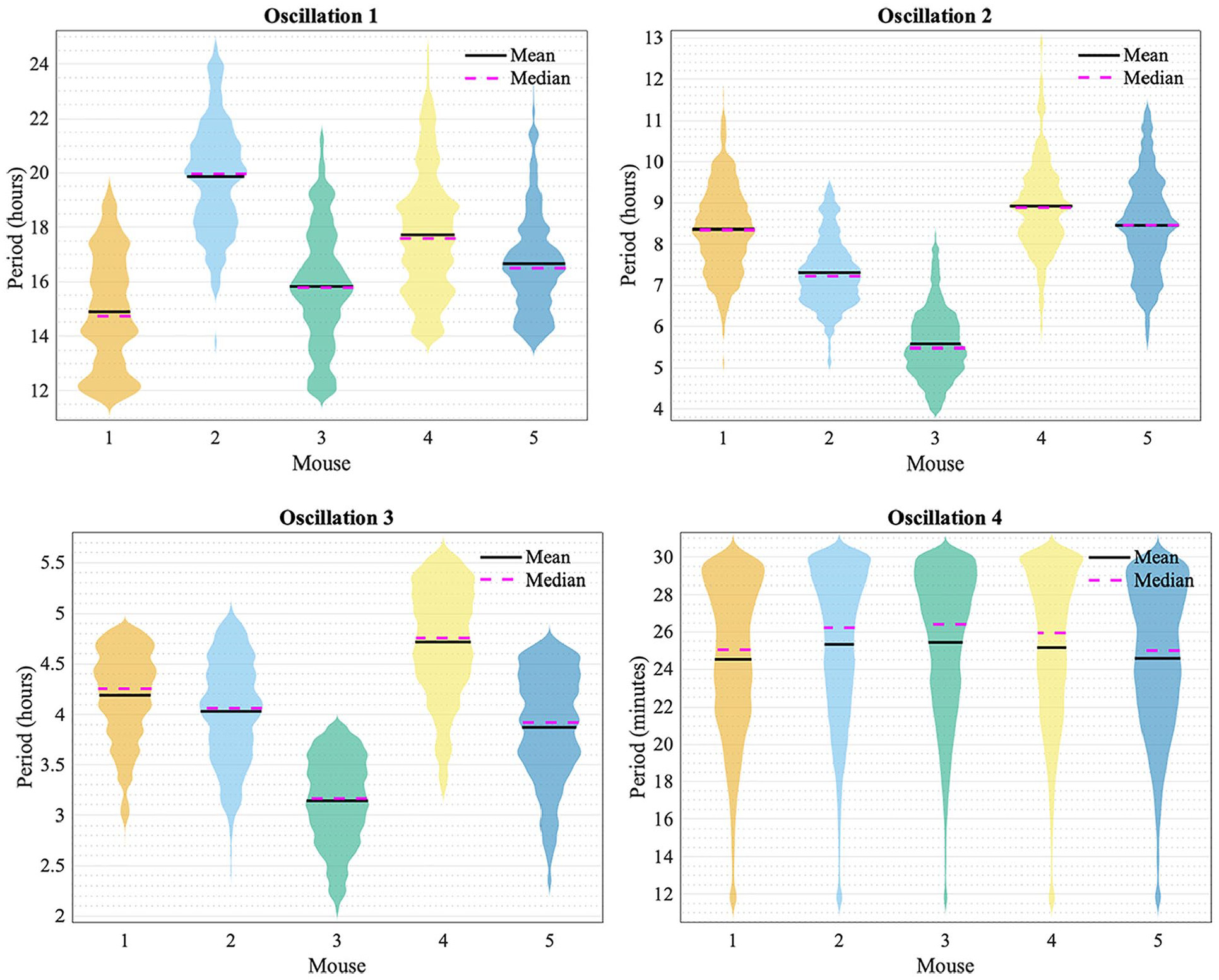
Violin plots for the periods of oscillation 1, 2, 3, and 4 for all mice (1, 2, 3, 4, and 5) obtained by the frequency ridges from ridge extraction.

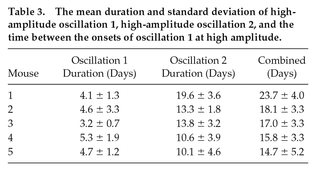
All the oscillatory components persist throughout data measurement, although the amplitudes of oscillations 1 and 2 are intermittently high and low, as can be seen in Figure 5. The amplitude of oscillation 2 decreases when the amplitude of oscillation 1 increases, and vice versa. A significant peak for oscillation 1 and oscillation 2 can be detected at all times, since the ridges can be extracted at all times. To investigate whether the high-amplitude appearance of oscillation 1 is common between all the mice, the start and end time for each appearance were noted. Figure 6 depicts the appearance of oscillation 1 for mouse 1, 2, 3, 4, and 5 (top to bottom), and the red lines are when the cages were changed. As can be seen, the appearance of oscillation 1 does not occur at the same time for all the mice, and does not occur as a result of changing the cages using an infrared light. Increasing the frequency of cage changes did not affect the appearance of oscillation 1. Furthermore, the mean frequency of oscillation 1 is not the same for all the mice. Therefore, it is unlikely there is a common external force driving the intermittent amplitude of oscillation 1. The time between the onsets of oscillation 1 at high amplitude appears rhythmic, and the mean times are given in Table 3 for all mice. Table 3 also gives the mean duration of high-amplitude oscillation 1 and high-amplitude oscillation 2.

Table 3.

The mean duration and standard deviation of high-amplitude oscillation 1, high-amplitude oscillation 2, and the time between the onsets of oscillation 1 at high amplitude.

Mouse	Oscillation 1 Duration (Days)	Oscillation 2 Duration (Days)	Combined (Days)
1	4.1 ± 1.3	19.6 ± 3.6	23.7 ± 4.0
2	4.6 ± 3.3	13.3 ± 1.8	18.1 ± 3.3
3	3.2 ± 0.7	13.8 ± 3.2	17.0 ± 3.3
4	5.3 ± 1.9	10.6 ± 3.9	15.8 ± 3.3
5	4.7 ± 1.2	10.1 ± 4.6	14.7 ± 5.2

Figure 5.

A smaller section of the time-frequency representation for mouse 2. Two oscillatory components appear intermittently. The blue lines show the boundaries for oscillation 1, and the red lines show the boundaries for oscillation 2. Oscillatory components between the blue and red lines, or by the bottom red line, are harmonics of the longer period oscillation. The vertical black dashed line marks where oscillation 1 decreases in amplitude and the other increases. The y-axis is presented on a logarithmic scale, and the “Wavelet power” is the squared amplitude of the wavelet and has units (wheel revolutions/min)².

Figure 6.

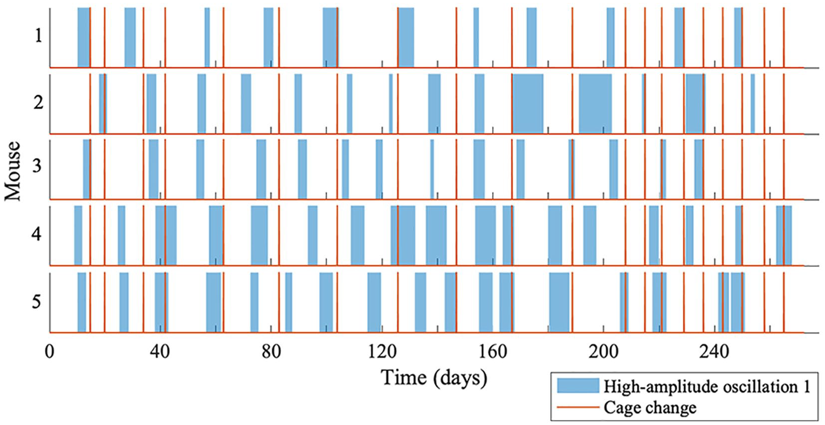
The appearance of oscillation 1 for mouse 1, 2, 3, 4, and 5. The periods when oscillation 1 is at high amplitude are shown by the blue blocks, and the red lines show cage changes.

Harmonics

By performing the harmonic finder algorithm for each mouse, the oscillatory components within harmonic relationships are made evident. The frequency interval investigated includes the entirety of the oscillatory components of interest: oscillation 1, 2, 3, and 4.

An example is shown in Figure 7 (harmonic results for the other mice data are shown in Suppl. Figs. S9-S12). The frequency boundaries used during ridge extraction for each oscillation detected in the time-frequency representation (oscillation 1, 2, 3, and 4) form the outlines of the dashed boxes in the figure. All the different combinations of oscillations are investigated, and the boxes are plotted over the harmonic results. For oscillation combinations which overlap with higher valued areas, the two oscillations are more likely in a harmonic relationship.

Figure 7.

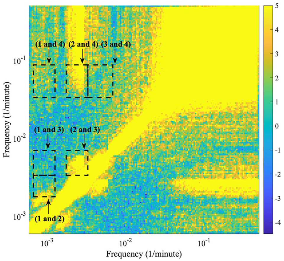
The detected harmonics within the behavioral data of mouse 2. The plot is a frequency-frequency representation showing what oscillations are in harmonic relationships. The image is symmetric over the diagonal; therefore, only half of the figure is considered. The frequency boundaries used during ridge extraction for each oscillation detected in the time-frequency representation (oscillation 1, 2, 3, and 4) form the outlines of the dashed boxes in the figure. All the different combinations of frequencies are investigated, and the boxes are plotted over the harmonic results. The color code shows a dimensionless quantity obtained from the actual value, minus the mean of the surrogate distribution, divided by the standard deviation of the surrogate distribution. Negative values correspond to results with values lower than the surrogate mean; therefore, significant results are those above 0. For oscillation combinations which overlap with higher valued areas, the two frequencies are more likely in a harmonic relationship.

For all mice, oscillation 1 and oscillation 3 do not appear to exist in a harmonic relationship. For mouse 1, 2, and 3, there is statistically significant evidence that oscillation 1 and oscillation 2 do not exist in a harmonic relationship; however, for mouse 4 and 5, oscillation 1 and oscillation 2 appear to exist in a harmonic relationship. For mouse 1, 2, 3, and 4, oscillation 2 and oscillation 3 exist in a harmonic relationship; however, for mouse 5, there is perhaps a faint signature of a harmonic relationship but it is not clear. Oscillation 1 and oscillation 4 do not appear to exist in a harmonic relationship, other than a possible faint signature in mouse 2 and 4. Oscillation 3 and 4 also do not appear to exist in a harmonic relationship, other than a possible faint signature in mouse 2 and 3. In all mice, oscillation 2 and oscillation 4 overlap with an area signifying a harmonic relationship; however, this area stretches to higher frequencies than the frequency interval surrounding the peak of oscillation 4.

A possible reason for oscillation 1 and oscillation 2 sometimes appearing as if they are in a harmonic relationship is due to the appearance of a harmonic of oscillation 1 just below oscillation 2. In Figure 7, a harmonic relationship exists below the oscillation 1 and oscillation 2 combination, corresponding to oscillation 1 and its harmonic. For mouse 4 and 5, oscillation 2 has a mean frequency similar to the harmonic of oscillation 1; therefore, it appears that oscillation 1 and oscillation 2 are in a harmonic relationship.

A harmonic relationship certainly exists in the region of oscillation 2 and oscillation 4 on the frequency-frequency representation, and the upper-frequency bound when extracting oscillation 4 may not be high enough. Therefore, it is highly probable that oscillation 2 and oscillation 4 are in a harmonic relationship.

In conclusion, oscillation 1 and oscillation 3 are not in a harmonic relationship. Oscillation 2 and oscillation 3 are highly probable in a harmonic relationship. Oscillation 1 and oscillation 2 are most likely not in a harmonic relationship, especially due to the harmonic relationship between oscillation 2 and oscillation 3, and lack of harmonic relationship between oscillation 1 and oscillation 3. Oscillation 1 and oscillation 4 are most likely not in a harmonic relationship, and similarly for oscillation 3 and oscillation 4. Oscillation 2 and oscillation 4 are highly probable in a harmonic relationship.

Coupling

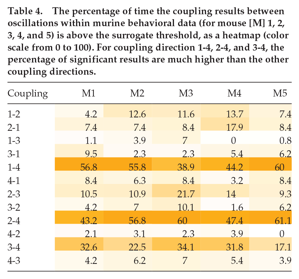
For each mouse, DBI was performed for all the possible combinations of pairs of oscillations (oscillation 1, 2, 3, and 4) obtained from the time-frequency representation by ridge extraction. From DBI, the coupling strength between two oscillations is obtained over time, for both directions of coupling.

Table 4.

The percentage of time the coupling results between oscillations within murine behavioral data (for mouse [M] 1, 2, 3, 4, and 5) is above the surrogate threshold, as a heatmap (color scale from 0 to 100). For coupling direction 1-4, 2-4, and 3-4, the percentage of significant results are much higher than the other coupling directions.

Coupling	M1	M2	M3	M4	M5
1-2	4.2	12.6	11.6	13.7	7.4
2-1	7.4	7.4	8.4	17.9	8.4
1-3	1.1	3.9	7	0	0.8
3-1	9.5	2.3	2.3	5.4	6.2
1-4	56.8	55.8	38.9	44.2	60
4-1	8.4	6.3	8.4	3.2	8.4
2-3	10.5	10.9	21.7	14	9.3
3-2	4.2	7	10.1	1.6	6.2
2-4	43.2	56.8	60	47.4	61.1
4-2	2.1	3.1	2.3	3.9	0
3-4	32.6	22.5	34.1	31.8	17.1
4-3	4.2	6.2	7	5.4	3.9

Table 5.

The mean coupling strength (×10⁻⁴) between oscillations within murine behavioral data (for mouse [M] 1, 2, 3, 4, and 5) when the coupling results are above the surrogate threshold, as a heatmap (color scale from 0 to 192). For coupling direction 1-4, 2-4, and 3-4, the mean coupling strengths are much higher than the other coupling directions. For mouse 4 coupling 1-3, and mouse 5 coupling 4-2, there were no significant results above the surrogate threshold.

Coupling	M1	M2	M3	M4	M5
1-2	18	23	28	43	22
2-1	16	15	13	21	12
1-3	22	34	38		22
3-1	12	11	14	9	10
1-4	192	171	146	181	176
4-1	12	9	10	10	10
2-3	23	36	42	29	34
3-2	15	20	26	15	16
2-4	164	176	167	153	169
4-2	11	17	12	29
3-4	158	161	145	178	153
4-3	18	27	32	16	19

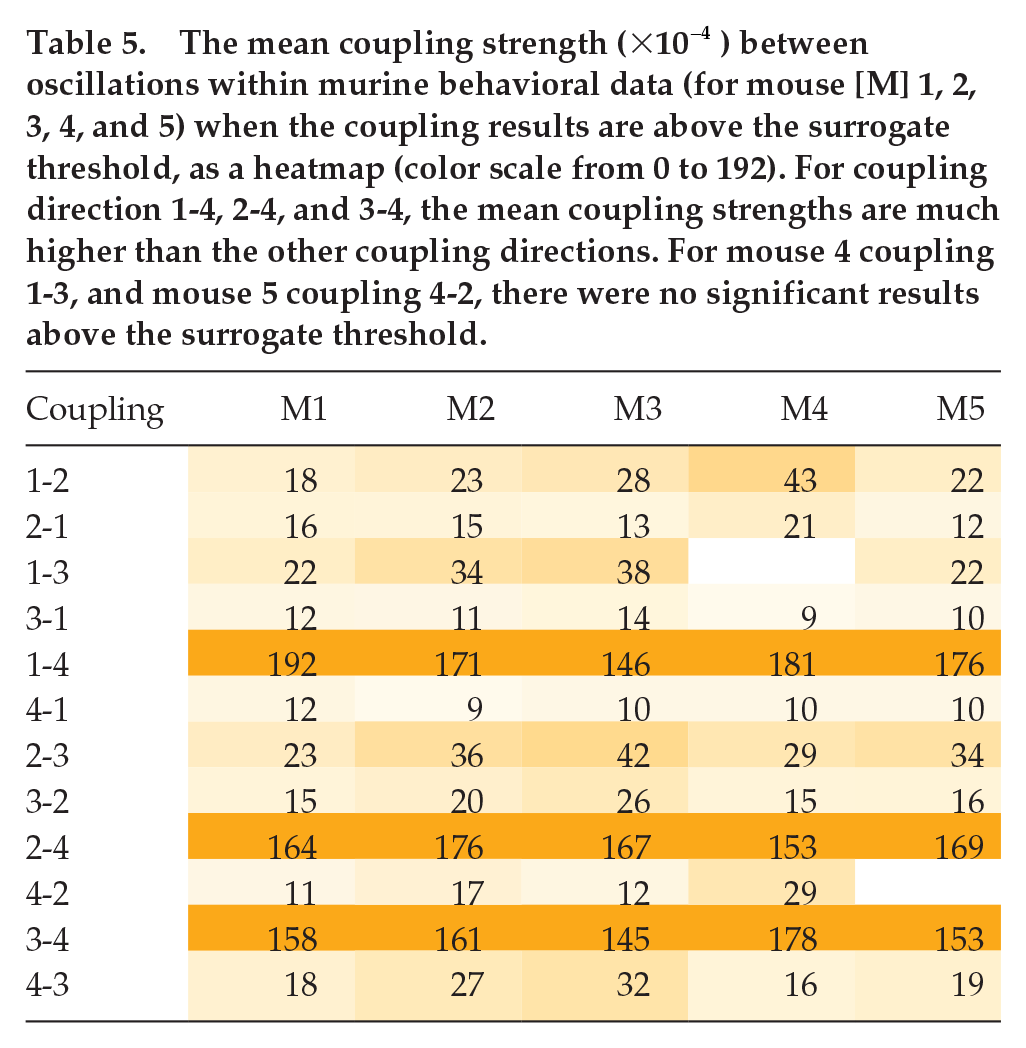
An example is shown in Figure 8 (DBI results for the other mice data are shown in Suppl. Figs. S13-S16). The solid lines denote the results from DBI using the pairs of phases, and the dotted lines are results obtained from surrogate data. Only values above the surrogate levels are considered as significant. Table 4 gives the percentage of time the coupling strengths from the phases are above the surrogate level, and Table 5 gives the mean coupling strength for the significant results. The coupling results are similar for all mice. There seems to be strong and stable (i.e. persists over time) coupling from oscillation 1, oscillation 2, and oscillation 3 to oscillation 4. There is some fluctuation around the surrogate line, perhaps due to oscillation 1 and oscillation 2 having time-varying phases, frequencies, and amplitudes. In the reverse direction, the coupling is less stable and weaker.

Figure 8.

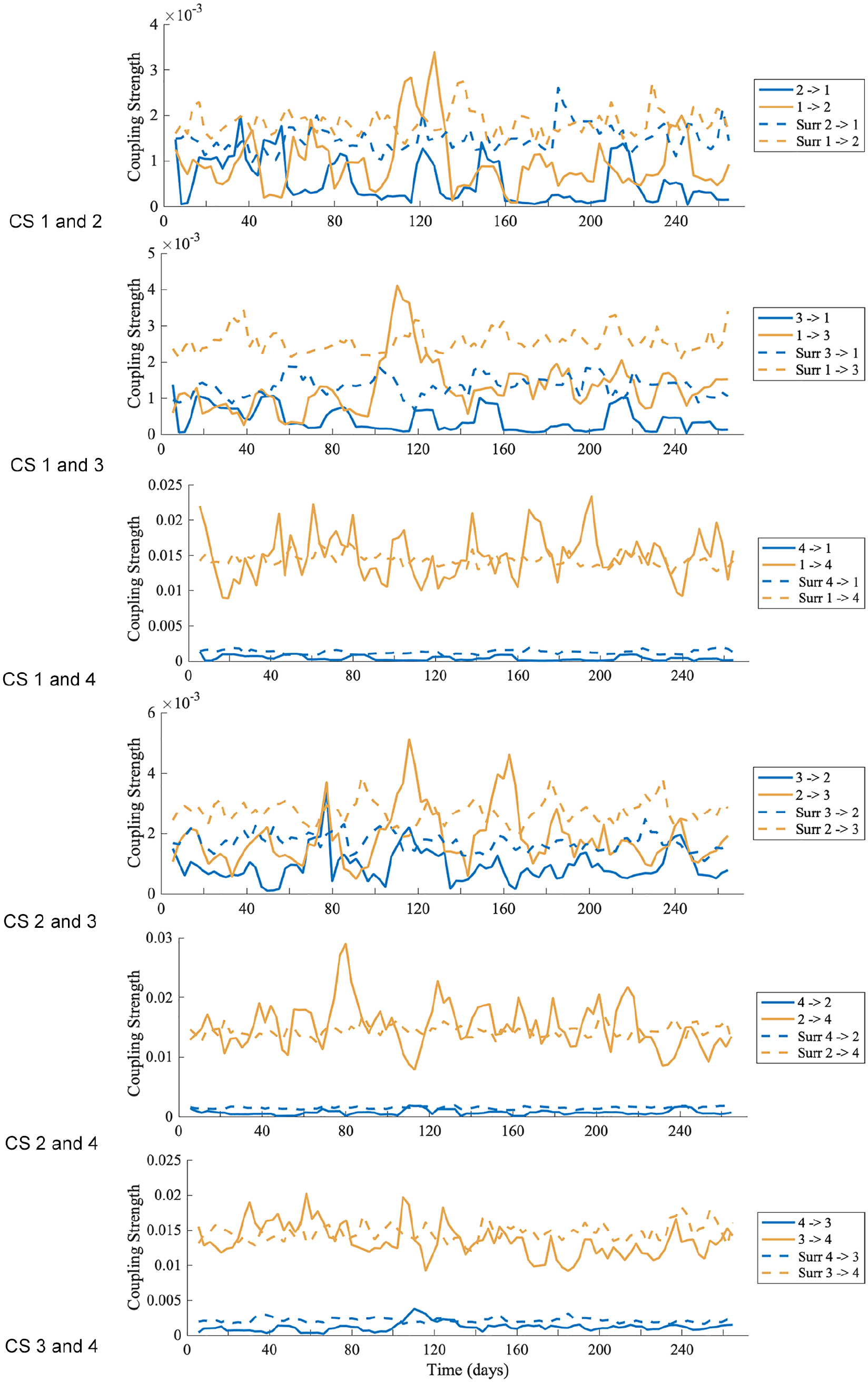
The coupling strength over time between four oscillations (oscillation 1, 2, 3, and 4), within the behavioral data of mouse 2. The solid lines denote the coupling strength results over time, obtained from dynamical Bayesian inference. The dotted lines are the surrogate significance tests. Only results above the surrogate lines are significant. The arrow in the legend denotes the direction of coupling.

The coupling between oscillation 1, oscillation 2, and oscillation 3 is weak, with the coupling stronger in the direction of oscillation 1 to oscillation 2 and oscillation 3 and stronger from oscillation 2 to oscillation 3, and is only present for a small percentage of time. A summary is given in Figure 9. An explanation for the intermittency of observed coupling is that it is a characteristic of nonautonomous systems (Lucas et al., 2018).

Figure 9.

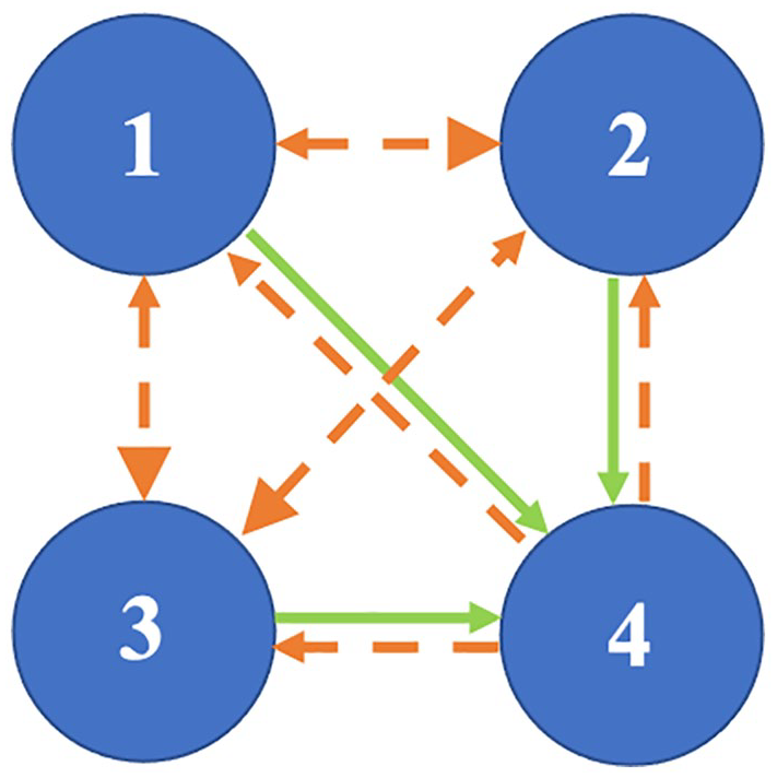
The coupling between the oscillations (1, 2, 3, and 4) within a murine biological system. There is strong and stable coupling from oscillation 1, oscillation 2, and oscillation 3 to oscillation 4, denoted by the solid green line, and weaker and less stable coupling from oscillation 4 to oscillation 1, oscillation 2, and oscillation 3, denoted by the dashed orange line. There is weak and less stable coupling between oscillation 1, oscillation 2, and oscillation 3, denoted by the dashed orange line, and the coupling is stronger from oscillation 1 to oscillation 2 and oscillation 3, and stronger from oscillation 2 to oscillation 3, denoted by the larger arrow head in these directions.

External Driver

By performing wavelet phase coherence for all possible pairs of mice, it is possible to determine whether there exists an external driver. This driver will then be common for all mice and will manifest as coherent oscillations at the same frequency for each pair.

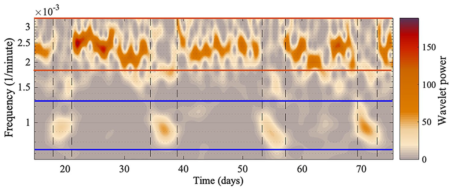
Accordingly, the median phase coherence for all mice is obtained. Four clusters of frequencies become evident, which are shown in Figure 10. The peaks within a cluster may be independent, or are perhaps due to time variations of a single oscillatory process. It can be seen that even after the removal of light and knocking out the genes responsible for the 24-h rhythm, there is still a common, approximately 24-h driver. In addition, peaks at 3.6 days, 1.8 days, and 21.6 h are observed, which based on simple division can be shown to be in a harmonic relationship, pointing to 3.6 days being the main external rhythm in addition to the 24-h rhythm. Most importantly, Figure 10 also illustrates that the behavioral rhythms summarized in Tables 1 and 2 are unlikely the result of an external driver, due to there being no significant peaks at the frequencies corresponding to the behavioral frequencies.

Figure 10.

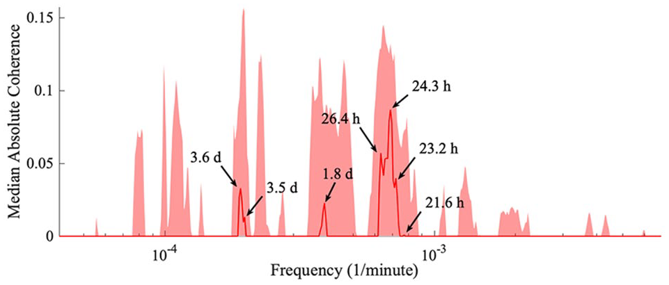
The median absolute coherence. After obtaining the wavelet phase coherence results for each pair of mice, the average phase coherence is calculated. The surrogate values were subtracted, and the median (red line) and 90th percentile (shaded red area) were determined across all the pairs of mice. Significant peaks correspond to an external driver synchronizing all the mice. Four frequency clusters arise, with peaks within a cluster possibly due to time variation.

With the chosen wavelet transform parameters, the minimum frequency is limited at $0.00004$ min⁻¹ or approximately $17$ days. Therefore, it is not possible to determine whether the intermittency between oscillator 1 and 2 is due to an external influence through wavelet phase coherence, due to the intermittency having a frequency around this limit. Although, from Figure 6, it is unlikely that the intermittency is due to an external driver, as discussed previously.

Discussion

Using 272 days of behavioral data sampled every 1 min from $P e r 1 / 2 / 3$ triple knockout mice kept in constant darkness, we have investigated the dynamics and interactions of the oscillatory components within the data. By applying the wavelet transform for time-localized frequency components with logarithmic frequency resolution, we observed that the intrinsic 24-h circadian rhythm is not visible; however, wavelet phase coherence revealed a common 24-h rhythm as an external driver, along with a 3.6-day external rhythm, both very weak. The wavelet transform did however reveal four prominent rhythmic components all less than 24 h, with periods of ∼17, ∼8, and ∼4 h, and ∼20 min. By implementing the harmonic finder algorithm, which is capable of detecting high harmonics in time-varying systems, we found that the ∼8- and ∼4-h rhythms and the ∼8- and ∼20-min rhythms were in a harmonic relationship. Due to the absence of external timing cues in our experimental setup, no known geophysical cycles of these periods, and a lack of phase coherence between mice in the ultradian range (Figure 10), we conclude that these ultradian rhythms are intrinsically driven. Coupling analysis of the ridge-extracted instantaneous frequencies revealed strong and frequent phase coupling from the slower oscillations (∼17, ∼8, and ∼4 h) to the faster oscillation (∼20 min), and weak and less frequent phase coupling in the reverse direction and between the slower oscillations.

Oscillation 1 and oscillation 2 have intermittent amplitude. When the amplitude of oscillation 1 increases, the amplitude of oscillation 2 decreases (and vice versa), and the cause for this is unknown. Bae and Weaver (2007) reported that a 3-h light pulse transiently induced a ∼16-h behavioral rhythm in Per1/2/3 triple knockout mice. Therefore, it is possible that a residual weak circadian oscillator exists in Per1/2/3 triple knockout mice and this (oscillation 1) is strengthened by an external force, for example, cage change, but the appearance of high-amplitude oscillation 1 was independent from the time the cages were changed (Figure 6). Moreover, oscillation 1 does not occur at the same time for all the mice, and the periods of the appearance of oscillation 1 varied between the mice (Table 3) and varied over time in each mouse. Oscillation 1 has a period similar to the extra-SCN circadian pacemakers in Per1/2/3 triple knockout mice (Flores et al., 2016; Pendergast et al., 2012); however, no procedure was performed to reveal behavioral rhythms driven by these oscillators. It is possible that oscillation 1 is strengthened by an internal, infradian mechanism; however, the purpose of such a biological oscillator is currently unclear.

The existence of an infradian oscillator and its connection with oscillation 1 and oscillation 2 remains to be investigated, and it is especially important to gain a good understanding of what internal or external events could activate oscillation 1 at high amplitude. Recently, Putker et al. (2021) have observed rhythms of a similar period to oscillation 1 in circadian gene Cry1/2 double knockout mice, which normally express arrhythmicity in constant darkness. A ∼16-h behavioral rhythm appeared when the cryptochrome-deficient mice were exposed to LL and then released to DD.

Robust ultradian rhythms of gene expression have been found by van der Veen and Gerkema (2016) in mouse liver tissue in vivo and NIH 3T3 cells in vitro from a 48-h dataset of hourly transcriptome measurements (Hughes et al., 2009; Barrett et al., 2013). Frequency peaks appear at $8$ and $12$ h; however, the prominent peak in vivo is at $12$ h and the prominent peak in vitro is at $8$ h. Although $8$ and $12$ h are harmonics of the circadian rhythm, the detection method disregards harmonics. Therefore, the gene expressions show true ultradian rhythms, disjoint from the circadian rhythm. From Tables 1 and 2, oscillation 2 is approximately $8$ h and may correspond to the in vitro results. Perhaps the difference between in vitro and in vivo is due to absence/presence of external information, with the presence of time givers, for example, the light-dark cycle and scheduled feeding times, elongating the period. The genes investigated show considerable variation in their expression patterns, with peaks occurring at different times. A significant amount of genes displaying ultradian expression patterns are associated with metabolic processes and the cell cycle. This could perhaps indicate a robust metabolic cycle, the like of which has been found in yeast (Tu et al., 2005). Rhythms of expression of yeast genes are found to have periods of the same length, ∼4-5 h. However, different genes follow different patterns of expression, with peaks occurring at different times. Therefore, the metabolic cycle is a highly organized expression cycle obtained through mutual coordination, leading to oxidative and reductive phases. The purpose of a metabolic cycle is to coordinate and temporally compartmentalize incompatible cellular processes which are essential to produce the energy needed for the working of the cell. Maintaining this underlying timekeeping mechanism is vital, in the absence or presence of external stimuli. For example, essential processes involved in the cell cycle are confined to the reductive phases to minimize oxidative damage to DNA. The metabolic cycle allows all necessary processes of a cell to take place at a time which optimizes the results. Hence, it is plausible to propose that oscillation 2 corresponds to a metabolic cycle. Interestingly, genes oscillating with ultradian frequencies appear to be those which emerged early in evolution (Castellana et al., 2018).

From our analysis, we see there is strong and stable coupling from longer rhythms (hours) to shorter rhythms (minutes). In mammalian cell biology, transcription occurs on a timescale of approximately 10 min (Shamir et al., 2016). Therefore, oscillation 4 may correspond to the vital processes that take place in the cell, which are driven by the metabolic cycle. Furthermore, ∼14-min neural activity rhythms were found both inside and outside the SCN of the hamster in constant darkness (Yamazaki et al., 1998).

To maintain synchrony between the metabolic cycles, there must exist cell-to-cell communication and coordination by a primary ultradian oscillator. Control by a central oscillator is supported by evidence such as that ultradian patterns of electrical activity in the brain are phase advanced compared with ultradian processes (Ootsuka et al., 2009). Various anatomical locations which seem to be essential for the generation, transmission, or coordination of ultradian rhythms have been discovered (Gerkema et al., 1990; Nakamura et al., 2008; Blum et al., 2014; Wu et al., 2018). The anatomical locations have appropriate connections for ultradian outputs and cross-talk with the circadian system (Goh et al., 2019).

To further elucidate the origin and mechanism of the ultradian rhythms, neural electrical activity could be measured via an EEG alongside collecting behavioral data of Per1/2/3 triple knockout mice kept in constant darkness. The dynamics and interactions of the oscillatory components that emerge can be investigated, along with the relationship between neural activity and behavior. For such a study, the minimum number of days of recording should include 8-10 cycles of the slowest oscillations under investigation. Therefore, investigating oscillation 1 would require at least 8-10 days of recording. However, due to the intermittent amplitude of oscillation 1 and oscillation 2, with a cycle of intermittency of around 20 days, a minimum recording of 160 days would be required.

By removing external perturbation such as light, and allowing the mice to feed, drink, and exercise ad libitum, the system may be modeled as approximately autonomous. However, there exists synchronization in the population, evincing other external perturbations. The rhythms that arise in Figure 10 could possibly be due to the variation of the Earth’s magnetic field (Courtillot and Le Mouel, 1988; Martynyuk and Temur’yants, 2009), which has a 24-h variation and 26- to 29-day variation; therefore, the third harmonic would lie in the range $3.25$ - $3.63$ days. How these rhythms affect the behavior of the mice is a further question, and whether they are causing the intermittency of oscillation 1 and oscillation 2. Subjecting the mice to varying magnetic field strengths and recording their behavior could further elucidate this hypothesis. The mice were physically separated; however, a coupling mechanism could exist through vocalizations and squeaky wheels resulting in social synchrony. The $3.6$ -days rhythm could be due to olfactory cues, for example, phermones which cue the estrous stage of female mice with a 4-day cycle, or is potentially a harmonic of the 7-day work cycle. The 24-h rhythm could be due to daily fluctuations of temperature or humidity fluctuations caused by air conditioning, or experimenter presence (noise, odor) in the animal facility. The coherence between temperature and humidity fluctuations and mouse behavior is shown in the Supplementary Material (Figs. S17 and S18). Weak, but significant peaks arise; however, they do not occur at the same frequencies for all mice. Mouse 2, 4, and 5 have a significant peak around ∼3.5 h and ∼53.0 min with temperature, and mouse 2, 3, 4, and 5 have a significant peak around ∼3.8 h with humidity (see Supplementary Material).

Although the sample size of this study is small, all the mice are characterized by a mutually consistent pattern, as illustrated in the Supplementary Material, Figures S1-S14. Furthermore, based on recordings of length 272 days, under constant conditions, we show that the pattern remains consistent over time. Thus, the nature and consistency of the results overcome the limitation of the relatively small sample size.

Diseases such as cancer can arise due to disruption of such biological rhythms, and comprehending their dynamics can be used to optimize drug delivery (Levi and Okyar, 2011). Given the importance of circadian and ultradian rhythms (McClung, 2007; Barger et al., 2009; van der Veen and Gerkema, 2016; Castellana et al., 2018), it is essential to gain an in-depth understanding of their nature. We have proposed a robust methodology that promises to open up new avenues to study a plethora of biological rhythms, including their dynamics and interactions, and possible ways of influencing these characteristics. Multiple, simultaneously recorded, time series of different physiological processes analyzed with the methodology described here could help to further investigate the origin of the rhythms and the mechanisms by which they influence each other.

Supplemental Material

sj-pdf-1-jbr-10.1177_07487304221087065 – Supplemental material for Multiscale Time-resolved Analysis Reveals Remaining Behavioral Rhythms in Mice Without Canonical Circadian Clocks

Supplemental material, sj-pdf-1-jbr-10.1177_07487304221087065 for Multiscale Time-resolved Analysis Reveals Remaining Behavioral Rhythms in Mice Without Canonical Circadian Clocks by Megan Morris, Shin Yamazaki and Aneta Stefanovska in Journal of Biological Rhythms

Footnotes

Acknowledgements

The article has come about as the result of a visit by AS to Auckland in the Spring of 2019. AS is grateful to Alona Ben-Tal for this invitation, for her splendid hospitality, for scientific discussions, and for the several introductions to New Zealand scientists. She gratefully acknowledges the Catalyst Fund Seeding provided by the New Zealand Ministry of Business, Innovation and Employment and administrated by the Royal Society Te Aprangi for supporting the visit. AS acknowledges stimulating discussions with Guy Warman and his group, and thanks him for the introduction to SY. This research was supported by a National Science Foundation grant IOS-1931115 and National Institute of Health grant R21 NS099809 to SY. The authors thank Alexandra J Brown for assistance with generating experimental mice and for animal care during behavior recording. MM thanks Lawrence Sheppard and Sam McCormack for helpful advice with algorithms and coding, and Juliane Bjerkan and Mansour Alanazi for running in parallel some of the computationally intensive algorithms. We are grateful to Julie Pendergast, and to the editor and anonymous referees for useful comments on the manuscript.

The development of MODA toolbox used for analyses has been supported by the Engineering and Physical Sciences Research Council (UK) Grant Nos. EP/100999X1 and EP/M006298/1], the EU projects BRACCIA [517133] and COSMOS [642563], the Action Medical Research (UK) MASDA Project [GN1963], and the Slovene Research Agency (Program No. P20232).

Conflict of Interest Statement

The author(s) have no potential conflicts of interest with respect to the research, authorship, and/or publication of this article.

Availability of Data and Codes

The data analyzed in this article are available on the Lancaster Publications and Research (Pure) system at (https://doi.org/10.17635/lancaster/researchdata/475), and the codes for the analysis methods used in this article are part of the toolbox MODA, which is available in MATLAB and Python at

ORCID iDs

Megan Morris

Shin Yamazaki

Aneta Stefanovska

Notes

References

Bae

Weaver

(2007) Transient, light-induced rhythmicity in mPER-deficient mice. J Biol Rhythms 22:85-88.

Bae

Jin

Maywood

Hastings

Reppert

Weaver

(2001) Differential functions of mPer1, mPer2, and mPer3 in the SCN circadian clock. Neuron 30:525-536.

Bandrivskyy

Bernjak

McClintock

Stefanovska

(2004) Wavelet phase coherence analysis: application to skin temperature and blood flow. Cardiovasc Eng 4:89-93.

Barger

Lockley

Rajaratnam

SMW

Landrigan

(2009) Neurobehavioral, health, and safety consequences associated with shift work in safety-sensitive professions. Curr Neurol Neurosci Rep 9:155-164.

Barrett

Wilhite

Ledoux

Evangelista

Kim

Tomashevsky

Marshall

Phillippy

Sherman

Holko

, et al. (2013) NCBI GEO: archive for functional genomics data sets: update. Nucleic Acids Res 41:991-995.

Bash

(1939) An investigation into a possible organic basis for the hunger drive. J Comp Psychol 28:109-135.

Blum

Zhu

Moquin

Kokoeva

Gratton

Giros

Storch

(2014) A highly tunable dopaminergic oscillator generates ultradian rhythms of behavioral arousal. eLife 3:e05105.

Brown

Pendergast

Yamazaki

(2019) Peripheral circadian oscillators. Yale J Biol Med 92:327-335.

Carmona

Hwang

Torresani

(1997) Characterization of signals by the ridges of their wavelet transforms. IEEE Trans Signal Process 45:2586-2590.

10.

Carmona

Hwang

Torresani

(1999) Multiridge detection and time-frequency reconstruction. IEEE Trans Signal Process 47:480-492.

11.

Castellana

Mazza

Capocefalo

Genov

Biagini

Fusilli

Scholkmann

Relógio

Hogenesch

Mazzoccoli

(2018) Systematic analysis of mouse genome reveals distinct evolutionary and functional properties among circadian and ultradian genes. Front Physiol 9:1178.

12.

Clemson

Stefanovska

(2014) Discerning non-autonomous dynamics. Phys Rep 542:297-368.

13.

Clemson

Lancaster

Stefanovska

(2016) Reconstructing time-dependent dynamics. Proc IEEE 104:223-241.

14.

Courtillot

Le Mouel

(1988) Time variations of the earth’s magnetic field: from daily to secular. Annu Rev Earth Planet Sci 16:389-476.

15.

Daubechies

(1992) Ten lectures on wavelets. Philadelphia (PA): Society for Industrial and Applied Mathematics.

16.

Delprat

Escudie

Guillemain

Kronland-Martinet

Tchamitchian

Torresani

(1992) Asymptotic wavelet and Gabor analysis: extraction of instantaneous frequencies. IEEE Trans Inform Theor 38:644-664.

17.

Dibner

Schibler

Albrecht

(2010) The mammalian circadian timing system: organization and coordination of central and peripheral clocks. Annu Rev Physiol 72:517-549.

18.

Dowse

Umemori

Koide

(2010) Ultradian components in the locomotor activity rhythms of the genetically normal mouse, Mus musculus. J Exp Biol 213:1788-1795.

19.

Dunlap

(1999) Molecular bases for circadian clocks. Cell 96:271-290.

20.

Flores

Bettilyon

Yamazaki

(2016) Period-independent novel circadian oscillators revealed by timed exercise and palatable meals. Sci Rep 6:21945.

21.

Foster

Hughes

Peirson

(2020) Circadian photoentrainment in mice and humans. Biology 9:180.

22.

Gerkema

Groos

Daan

(1990) Differential elimination of circadian and ultradian rhythmicity by hypothalamic lesions in the common vole, Microtus arvalis. J Biol Rhythms 5:81-95.

23.

Goh

Maloney

Mark

Blache

(2019) Episodic ultradian events – ultradian rhythms. Biology 8:15.

24.

Grinsted

Moore

Jevrejeva

(2004) Application of the cross wavelet transform and wavelet coherence to geophysical time series. Nonlin Processes Geophys 11:561-566.

25.

Hastings

Maywood

Brancaccio

(2018) Generation of circadian rhythms in the suprachiasmatic nucleus. Nat Rev Neurosci 19:453-469.

26.

Hoffmann

(2015) violin.m: simple violin plot using matlab default kernel density estimation. Bonn, Germany: Institute of Crop Science and Resource Conservation, University of Bonn.

27.

Hughes

DiTacchio

Hayes

Vollmers

Pulivarthy

Baggs

Panda

Hogenesch

(2009) Harmonics of circadian gene transcription in mammals. PLoS Genet 5:e1000442.

28.

Iatsenko

McClintock

PVE

Stefanovska

(2015) Linear and synchrosqueezed time-frequency representations revisited: overview, standards of use, resolution, reconstruction, concentration, and algorithms. Digit Signal Process 42:1-26.

29.

Iatsenko

McClintock

PVE

Stefanovska

(2016) Extraction of instantaneous frequencies from ridges in time-frequency representations of signals. Signal Process 125:290-303.

30.

Jensen

Colgin

(2007) Cross-frequency coupling between neuronal oscillations. Trends Cogn Sci 11:267-269.

31.

Kaiser

(1994) A friendly guide to wavelets. Birkhäuser Boston. https://link.springer.com/book/10.1007/978-0-8176-8111-1#about

32.

Kippert

Hunt

(2000) Ultradian clocks in eukaryotic microbes: from behavioural observation to functional genomics. BioEssays 22:16-22.

33.

Kloeden

Rasmussen

(2011) Nonautonomous dynamical systems. Providence (RI): American Mathematical Society.

34.

Kloeden

Yang

(2020) An introduction to nonautonomous dynamical systems and their attractors. Singapore: World Scientific Publishing.

35.

Lachaux

Lutz

Rudrauf

Cosmelli

Le Van Quyen

Martinerie

Varela

(2002) Estimating the time-course of coherence between single-trial brain signals: an introduction to wavelet coherence. Neurophysiol Clin 32:157-174.

36.

Lancaster

Iatsenko

Pidde

Ticcinelli

Stefanovska

(2018) Surrogate data for hypothesis testing of physical systems. Phys Rep 748:1-60.

37.

LeGates

Fernandez

Hattar

(2014) Light as a central modulator of circadian rhythms, sleep and affect. Nat Rev Neurosci 15:443-454.

38.

Le Van Quyen

Foucher

Lachaux

Rodriguez

Lutz

Martinerie

Varela

(2001) Comparison of Hilbert transform and wavelet methods for the analysis of neuronal synchrony. Neurosci Methods 111:83-98.

39.

Lévi

Okyar

(2011) Circadian clocks and drug delivery systems: impact and opportunities in chronotherapeutics. Expert Opin Drug Deliv 8:1535-1541.

40.

Lucas

Newman

Stefanovska

(2018) Stabilization of dynamics of oscillatory systems by nonautonomous perturbation. Phys Rev E 97:042209.

41.

Martynyuk

Temur’yants

(2009) Extremely low frequency magnetic fields as a modulation factor and synchronization of infradian biorhythms in animals. Geofiz Protsessy Biosfera 8:36-50.

42.

McClung

(2007) Circadian genes, rhythms and the biology of mood disorders. Pharmacol Ther 114:222-232.

43.

Mohawk

Baer

Menaker

(2009) The methamphetamine-sensitive circadian oscillator does not employ canonical clock genes. Proc Natl Acad Sci U S A 106:3519-3524.

44.

Morse

Sassone-Corsi

(2002) Time after time: inputs to and outputs from the mammalian circadian oscillators. Trends Neurosci 25:632-637.

45.

Nakamura

Yamazaki

Nakamura

Shirakawa

Block

Takumi

(2008) In vivo monitoring of circadian timing in freely moving mice. Curr Biol 18:381-385.

46.

Newman

Lancaster

Stefanovska

(2018) Multiscale oscillatory dynamics analysis (v1.01, user manual). https://www.matrix-inst.org.au/wp_Matrix2016/wp-content/uploads/2019/2019_07_Angelova/MODA-User-Manual.pdf.

47.

Newman

Lucas

Stefanovska

(2021) Stabilization of cyclic processes by slowly varying forcing. Chaos 31:123129.

48.

Ootsuka

de Menezes

Zaretsky

Alimoradian

Hunt

Stefanidis

Oldfield

Blessing

(2009) Brown adipose tissue thermogenesis heats brain and body as part of the brain-coordinated ultradian basic rest-activity cycle. Neuroscience 164:849-861.

49.

Paluš

Stefanovska

(2003) Direction of coupling from phases of interacting oscillators: an information-theoretic approach. Phys Rev E 67:055201.

50.

Pendergast

Yamazaki

(2017) Extra-SCN circadian pacemakers. In: Honma

Honma

editors. Biological Clocks with Reference to Suprachiasmatic Nucleus: Proceedings of the Sapporo Symposium on Biological Rhythm November 9-10, 2016. Sapporo (Japan): Hokkaido University Press. p. 141-152.

51.

Pendergast

Friday

Yamazaki

(2009) Endogenous rhythms in Period1 mutant suprachiasmatic nuclei in vitro do not represent circadian behavior. J Neurosci 29:14681-14686.

52.

Pendergast

Friday

Yamazaki

(2010) Distinct functions of Period2 and Period3 in the mouse circadian system revealed by in vitro analysis. PLoS ONE 5:e8552.

53.

Pendergast

Oda

Niswender

Yamazaki

(2012) Period determination in the food-entrainable and methamphetamine-sensitive circadian oscillator(s). Proc Natl Acad Sci U S A 109:14218-14223.

54.

Putker

Wong

DCS

Seinkmane

Rzechorzek

Zeng

Hoyle

Chesham

Edwards

Feeney

Fischer

, et al. (2021) CRYPTOCHROMES confer robustness, not rhythmicity, to circadian timekeeping. EMBO J 25:e106745.

55.

Rosenblum

Pikovsky

(2001) Detecting direction of coupling in interacting oscillators. Phys Rev E 64:045202.

56.

Shamir

Bar-On

Phillips

Milo

(2016) SnapShot: timescales in cell biology. Cell 164:1302.

57.

Shearman

Jin

Lee

Reppert

Weaver

(2000) Targeted disruption of the mPer3 gene: subtle effects on circadian clock function. Mol Cell Biol 20:6269-6275.

58.

Shearman

Sriram

Weaver

Maywood

Chaves

Zheng

Kume

Lee

van der Horst

GTJ

Hastings

, et al. (2000) Interacting molecular loops in the mammalian circadian clock. Science 288:1013-1019.

59.

Sheppard

Stefanovska

McClintock

PVE

(2011) Detecting the harmonics of oscillations with time-variable frequencies. Phys Rev E 83:016206.

60.

Sheppard

Stefanovska

McClintock

PVE

(2012) Testing for time-localized coherence in bivariate data. Phys Rev E 85:046205.

61.

Smelyanskiy

Luchinsky

Stefanovska

McClintock

PVE

(2005) Inference of a nonlinear stochastic model of the cardiorespiratory interaction. Phys Rev Lett 94:098101.

62.

Stankovski

Duggento

McClintock

PVE

Stefanovska

(2012) Inference of time-evolving coupled dynamical systems in the presence of noise. Phys Rev Lett 109:024101.

63.

Stankovski

Duggento

McClintock

PVE

Stefanovska

(2014) A tutorial on time-evolving dynamical Bayesian inference. Eur Phys J Spec 223:2685-2703.

64.

Stankovski

Pereira

McClintock

PVE

Stefanovska

(2017) Coupling functions: universal insights into dynamical interaction mechanisms. Rev Mod Phys 89:045001.

65.

Stankovski

Pereira

McClintock

PVE

Stefanovska

(2019) Coupling functions: dynamical interaction mechanisms in the physical, biological and social sciences. Phil Trans R Soc A 377:20190039.

66.

Stefanovska

McClintock

PVE

, and editors (2021) Physics of biological oscillators: new insights into non-equilibrium and non-autonomous systems. Cham: Springer.

67.

Stephenson

Lim

Famina

Caron

Dowse

(2012) Sleep-wake behavior in the rat: ultradian rhythms in a light-dark cycle and continuous bright light. J Biol Rhythms 27:490-501.

68.

Storch

Weitz

(2009) Daily rhythms of food-anticipatory behavioral activity do not require the known circadian clock. Proc Natl Acad Sci U S A 106:6808-6813.

69.

Suprunenko

Clemson

Stefanovska

(2013) Chronotaxic systems: a new class of self-sustained nonautonomous oscillators. Phys Rev Lett 111:024101.

70.

Kudlicki

Rowicka

McKnight

(2005) Logic of the yeast metabolic cycle: temporal compartmentalization of cellular processes. Science 310:1152-1158.

71.

van der Veen

Gerkema

(2016) Unmasking ultradian rhythms in gene expression. FASEB J 31:743-750.

72.

Waite

McKenna

Kershaw

Walker

Cho

Piggins

Lightman

(2012) Ultradian corticosterone secretion is maintained in the absence of circadian cues. Eur J Neurosci 36:3142-3150.

73.

Weaver

(1998) The suprachiasmatic nucleus: a 25-year retrospective. J Biol Rhythms 13:100-112.

74.

Enoki

Oda

Huang

Honma

(2018) Ultradian calcium rhythms in the paraventricular nucleus and subparaventricular zone in the hypothalamus. Proc Natl Acad Sci U S A 115:9469-9478.

75.

Yamazaki

Kerbeshian

Hocker

Block

Menaker

(1998) Rhythmic properties of the hamster suprachiasmatic nucleus in vivo. J Neurosci 18:10709-10723.

Supplementary Material

Please find the following supplemental material available below.

For Open Access articles published under a Creative Commons License, all supplemental material carries the same license as the article it is associated with.

For non-Open Access articles published, all supplemental material carries a non-exclusive license, and permission requests for re-use of supplemental material or any part of supplemental material shall be sent directly to the copyright owner as specified in the copyright notice associated with the article.

0.00 MB

6.96 MB

Coupling	M1	M2	M3	M4	M5
1-2	18	23	28	43	22
2-1	16	15	13	21	12
1-3	22	34	38		22
3-1	12	11	14	9	10
1-4	192	171	146	181	176
4-1	12	9	10	10	10
2-3	23	36	42	29	34
3-2	15	20	26	15	16
2-4	164	176	167	153	169
4-2	11	17	12	29
3-4	158	161	145	178	153
4-3	18	27	32	16	19

Coupling	M1	M2	M3	M4	M5
1-2	18	23	28	43	22
2-1	16	15	13	21	12
1-3	22	34	38		22
3-1	12	11	14	9	10
1-4	192	171	146	181	176
4-1	12	9	10	10	10
2-3	23	36	42	29	34
3-2	15	20	26	15	16
2-4	164	176	167	153	169
4-2	11	17	12	29
3-4	158	161	145	178	153
4-3	18	27	32	16	19

Coupling	M1	M2	M3	M4	M5
1-2	18	23	28	43	22
2-1	16	15	13	21	12
1-3	22	34	38		22
3-1	12	11	14	9	10
1-4	192	171	146	181	176
4-1	12	9	10	10	10
2-3	23	36	42	29	34
3-2	15	20	26	15	16
2-4	164	176	167	153	169
4-2	11	17	12	29
3-4	158	161	145	178	153
4-3	18	27	32	16	19