
Abstract
Circadian rhythms provide daily temporal structure to cellular and organismal biological processes, ranging from gene expression to cognition. Higher-frequency (intradaily) ultradian rhythms are similarly ubiquitous but have garnered far less empirical study, in part because of the properties that define them—multimodal periods, non-stationarity, circadian harmonics, and diurnal modulation–pose challenges to their accurate and precise quantification. Wavelet analyses are ideally suited to address these challenges, but wavelet-based measurement of ultradian rhythms has remained largely idiographic. Here, we describe novel analytical approaches, based on discrete and continuous wavelet transforms, which permit quantification of rhythmic power distribution across a broad ultradian spectrum, as well as precise identification of period within empirically determined ultradian bands. Moreover, the aggregation of normalized wavelet matrices allows group-level analyses of experimental treatments, thereby circumventing limitations of idiographic approaches. The accuracy and precision of these wavelet analyses were validated using in silico and in vivo models with known ultradian features. Experiments in male and female mice yielded robust and repeatable measures of ultradian period and power in home cage locomotor activity, confirming and extending reports of ultradian rhythm modulation by sex, gonadal hormones, and circadian entrainment. Seasonal changes in day length modulated ultradian period and power, and exerted opposite effects in the light and dark phases of the 24 h day, underscoring the importance of evaluating ultradian rhythms with attention to circadian phase. Sex differences in ultradian rhythms were more prominent at night and depended on gonadal hormones in male mice. Thus, relatively straightforward modifications to the wavelet procedure allowed quantification of ultradian rhythms with appropriate time-frequency resolution, generating accurate, and repeatable measures of period and power which are suitable for group-level analyses. These analytical tools may afford deeper understanding of how ultradian rhythms are generated and respond to interoceptive and exteroceptive cues.
Keywords
Biological rhythmicity is a fundamental property of all living systems (Edgar et al., 2012; Bloch et al., 2013) with implications for many fields of biology (Bloch et al., 2013; Ramp et al., 2015; Wang et al., 2015; Evans and Gorman, 2016; Spoelstra et al., 2016; Turek, 2016; Riede et al., 2017). Circadian rhythms (CRs), which evolved to anticipate regularly recurring cycles tied to the ~24 h rotation of the earth about its axis, have been studied extensively, and their relevance to regulatory biology and human health is well-established (Savvidis and Koutsilieris, 2012; Evans and Davidson, 2013; Stevenson et al., 2015; Walker et al., 2020; Zheng et al., 2020).
In contrast, intradaily (1-6 h) ultradian rhythms (URs) are relatively understudied (Prendergast and Zucker, 2016; Grant et al., 2018). This is surprising, given that the influence of URs on physiology and behavior appears as pervasive as that of CRs: URs manifest in countless behavioral and physiological processes important for homeostasis (e.g., food consumption, water intake, sleep, body temperature, metabolic gene expression, hormone secretion, among others) in diverse species (Stavreva et al., 2009; Bloch et al., 2013; Blessing and Ootsuka, 2016; Prendergast and Zucker, 2016; Bourguignon and Storch, 2017; van der Veen and Gerkema, 2017; Aviram et al., 2021). Changes in the temporal properties of URs have also been associated with major life history events (e.g., ovulation, pregnancy, lactation; Prendergast et al., 2012a; Smarr et al., 2016) and with the progression of disease (Smarr et al., 2019). Ultradian patterns of hormone release are required to elicit normal pituitary activity (Belchetz et al., 1978) and gene transcription (Stavreva et al., 2009; McMaster et al., 2011). And finally, URs are sexually differentiated (Prendergast and Zucker, 2016), exhibiting phenotypic plasticity in response to endogenous (Painson and Tannenbaum, 1991) and exogenous changes in gonadal hormones (rats: (Wollnik and Turek, 1988), hamsters: (Prendergast et al., 2012a, 2012b; Wang et al., 2014), mice: (Smarr et al., 2017)) and gonadectomy (Daan et al., 1975; Wollnik and Dohler, 1986). Sex- and hormone-mediated changes in URs also manifest more prominently in specific phases of the circadian cycle (Daan et al., 1975; Wollnik and Dohler, 1986; Wollnik and Turek, 1988; Prendergast et al., 2012a; Wang et al., 2014; Smarr et al., 2017). Despite these many commonalities, the mechanisms by which sex, gonadal hormones, and the circadian system interact with URs are not fully characterized.
Several differences between URs and CRs present obstacles to more extensive investigation. First, URs are not linked to any known astrophysical periodicity (e.g., planetary rotation or orbit), and thus there is no a priori expected period value for any given UR. Indeed, URs exhibit complex waveforms, often with more than one ultradian periodicity expressed depending on the time of day, thus the specification of a single period is not always applicable to URs. Second, neural substrates of URs have proven difficult to localize, and it is unclear whether individual URs are controlled by distinct substrates (Miyata et al., 2016; Prendergast and Zucker, 2016; Bourguignon and Storch, 2017; Grant et al., 2018; Wu et al., 2018). Third, URs appear to change over the circadian cycle, but any role of the circadian system in the generation and expression of URs is likely complex: an intact circadian oscillator is not required for the expression of URs, for example, and URs persist following physical (Gerkema et al., 1990; Gerkema and van der Leest, 1991; Gerkema et al., 1993; Blum et al., 2014), chemical (Blum et al., 2014) and genomic (Vitaterna et al., 1994; Zheng et al., 1999; Bunger et al., 2000; Zheng et al., 2001; Abraham et al., 2006) manipulations of the circadian pacemaker, yet circadian transitions between locomotor activity and rest robustly modulate the UR waveform (Smarr et al., 2017). URs exhibit remarkable plasticity as the circadian system entrains to seasonal changes in photoperiod: under short (winter) photoperiods nocturnal locomotor activity URs of mice (Refinetti, 2002), hamsters (Prendergast and Zucker, 2012), and rats (Siebert and Wollnik, 1991) become more prominent. In the field, when extremely long and short photoperiods prevail, arctic species (e.g., reindeer, ptarmigan) largely abandon CRs in favor of robust URs (van Oort et al., 2007; Bloch et al., 2013; Appenroth et al., 2021), challenging the hegemony of circadian rhythmicity (Hazlerigg and Tyler, 2019).
A final and critical dissimilarity is that URs must be quantified differently than CRs. Individuals commonly exhibit multiple URs simultaneously (e.g., locomotor activity, hormone pulsatility) (Bourguignon and Storch, 2017; Grant et al., 2018), with a broader normative period range than CRs, that tend to co-occur around circadian harmonics. URs are non-stationary, varying in period/phase, waveform, and amplitude from cycle to cycle (Refinetti et al., 2007). Harmonics, non-stationarity, and multiple periodicities each pose substantial challenges to Fourier-based methods that are typically used to extract quantitative metrics (period/phase, power) from CRs, and thus these quantitative methods are not ideal for measuring URs (Leise, 2017).
The continuous wavelet transform surmounts many of these obstacles and provides a desirable alternative technique for quantification, by generating a scalogram (a spectrogram-like representation of the underlying signal (Leise, 2013)) which is robust to non-stationarity and has time-frequency resolution sufficient to accurately identify URs even in the face of circadian harmonic contamination (Leise and Harrington, 2011; Leise, 2013). Continuous wavelet transform scalograms are highly informative, but in common with circadian actograms, are also highly individualistic. The presence of multiple UR periods within individual scalograms, together with the modulation of URs over circadian timescales, precludes simply collapsing UR scalograms across many individuals to develop measures of central tendency and perform group-level parametric statistical analyses. Consequently, wavelet-derived information on URs is often idiographic, restricted to representative-animal illustrations, (Leise and Harrington, 2011; Blum et al., 2014; Miyata et al., 2016; Wu et al., 2018; Goh et al., 2019), or systems level analyses (Smarr et al., 2019). Given the emerging interest in ultradian biology over the past decade (Bloch et al., 2013; Blum et al., 2014; Prendergast et al., 2015; Miyata et al., 2016; Smarr et al., 2016; Grant et al., 2018; Wu et al., 2018; Hazlerigg and Tyler, 2019; Grant et al., 2020; Appenroth et al., 2021; Aviram et al., 2021; van Rosmalen and Hut, 2021), resolving such limitations may provide useful new research methods for the field.
Here, we report and extensively validate, using in silico models with known ultradian periods, straightforward modifications to wavelet analysis procedures which address many of the challenges posed by URs. Reduction of the complex wavelet scalogram into discrete estimates of power (across periods) and period (within objectively defined power bands) permitted aggregation of data across individual subjects for group-level analyses. These modifications allow for several benefits over existing wavelet applications for the study of behavior: measurement of URs during distinct phases of the circadian cycle, specification of peak period values within discrete bands of the UR spectrum, and aggregation of UR measures across individuals within treatment groups. Additional experiments then evaluated the accuracy, repeatability, and precision of these analytical methods in vivo, by quantifying URs of female and male mice following genomic, hormonal, and environmental manipulations previously reported to alter URs. The approaches described here supplement existing wavelet methods and may permit novel analyses of CR and UR interactions.
General Methods
Animals and Housing
Male and female mice for all experiments were obtained from Jackson Laboratory (Bar Harbor, ME, USA). WT mice were on backgrounds of (C57BL/6 J [JAX Catalog #: 000664; black coat color] or B6(Cg)-Tyrc-2 J/J [JAX Catalog #: 000058; albino color]). Mutant mice in Experiment 1 homozygous for the Per2Brdm1 mutation [JAX Catalog #: 003819; Per2 m/m ] were ordered directly from Jackson Labs (Riggle et al., 2022). Mice were housed in an intermediate-duration photoperiod that provided 12 h light and 12 h darkness each day (12 L:12D; ‘intermediate days’), with the exception of Experiment 3 (see Photoperiod manipulations). Experiments were performed on adult mice; see specific Experiments for ages and sample sizes. Estrous cycles of females were not monitored. Mice were housed in polypropylene cages (28 cm × 17 cm × 12 cm) on irradiated corncob bedding (Irradiated 1/8” Corn Cobs, Envigo, Indianapolis, IN, USA). Ambient temperature and relative humidity were monitored and maintained at 20 ± 0.5 °C and 53% ± 2%, respectively. Food (Teklad Global 18% Protein Rodent Diet 2918, Envigo); filtered tap water and cotton nesting material were continuously available in the cages. All experimental procedures conformed to the National Institutes of Health (NIH) Guidelines for the Care and Use of Laboratory Animals and were approved by the Institutional Animal Care and Use Committee of the University of Chicago.
Locomotor Activity Monitoring
In all experiments, home cage locomotor activity was continuously monitored with passive infrared motion detectors mounted outside the cage, ~22 cm above the cage floor. Motion detectors registered locomotor activity via closure of an electronic relay, recorded by a computer running Clocklab software (Actimetrics; Evanston, IL, USA). Cumulative locomotor activity counts were binned at 1 min intervals. URs and CRs were quantified from 10-day epochs of locomotor activity (described below).
Photoperiod Manipulations
Animal housing rooms were illuminated with overhead fluorescent lighting (~400 lux at the level of the cage lid). Digital timers controlled lights to deliver 1 of 3 static lighting cycles (photoperiods): 12 L:12D (an intermediate photoperiod), 16 L:8D (a long photoperiod), and 8 L:16D (a short photoperiod). Increases and decreases in photoperiod duration were accomplished by symmetrical expansion and compression, respectively, of the light phase (i.e., the midpoint of the light phase always remained the same). Per2 m/m mutant mice used in Experiment 1.3 were also exposed to continuous darkness (DD) and a 2 L:2D photocycle. Mouse husbandry in DD was facilitated via dim handheld red illumination (< 1 lux), otherwise mice were maintained in complete darkness.
Circadian Locomotor Activity Analyses
Circadian entrainment was confirmed via qualitative analysis of double-plotted actograms (Figure 4A), which were generated in Clocklab software (v. 2.56; Actimetrics, Evanston, IL, USA). Fourier-based quantitative evaluation of CRs was performed using a Lomb-Scargle periodogram analysis in MATLAB (Mathworks), which estimates a frequency spectrum by using a least-squared method of fitting the locomotor activity time series to a series of sinusoids. The Lomb-Scargle periodogram is a common and well-established analytical technique for the evaluation of rhythmic circadian signals (Refinetti et al., 2007; Tackenberg and Hughey, 2021).
Pre-Processing
Post-collection data quality assessment was performed in MATLAB: infrequent data dropouts (transcription errors, corrupted data points; encoded as ‘NaN’) were substituted with values equal to a 10-min moving average. In instances where this failed, values were substituted with zero. To remove the influence of outlier data points in the time series, any value exceeding 4x the standard deviation of the time series was replaced with a value equal to 4x the standard deviation of the time series. On occasion, larger, multi-day data dropouts occurred because of passive infrared sensor malfunction on a channel, in which case that channel was excluded from the affected 10-day analysis window. Final sample sizes are reported in each experimental section below and in figure legends. In mice exposed to short days, a computer failure during the week 6 data collection interval resulted in one day of incomplete data for all animals. In order to obtain a complete 10 days of data for this analysis interval, data collection was extended by one additional day, and the data from the day of the computer failure were excised.
Parsing
Locomotor activity data from each mouse were first separated into light or dark phase components (diurnal parsing). Parsing was performed prior to wavelet transformations, and did not generate artifacts or spurious ultradian periods to emerge from the analysis, as confirmed via simulations (see Experiment 1.1, and Figure 2A and 2C). Light and dark phase activity data were then each individually subjected to the continuous wavelet transform, which produced scalogram matrices for each record.
Wavelet Analyses
When applied to time series data, wavelets identify harmonics and are robust to non-stationarity because they evaluate the time series over only very small and narrowly defined windows in which it is far more likely to be stationary; the latter is especially useful in more accurately resolving ultradian components. Prior work has demonstrated the robustness of wavelet approaches to circadian harmonics in simulated and real activity records of individual subjects (Leise, 2013). We acknowledge that harmonic contamination likely exists in the present data, but, consistent with prior observations, the results obtained here did not appear to be dominated by circadian harmonics, despite the presence of a high-amplitude 24 h signal in the simulated and actual data. Instead, wavelet analyses recovered either known ultradian periodicities (from simulation and Per2 m/m data) or group means that varied by sex, gonadal status, photocycle, or time. For additional background and a focused discussion of the merits and limitations of wavelet-based time series analyses in the measurement of behavioral rhythmicity, see reviews (Leise and Harrington, 2011; Leise, 2013, 2015, 2017). We identified a generalized Morse wavelet of γ = 3 and β = 10 to provide suitable time-frequency resolution for our experimental data (i.e., C57BL6/J mice, recorded via passive infrared motion detectors). β serves as a toggle of temporal and frequency resolution. Increasing β increases the sharpness of peaks seen in the power versus period plots but reduces temporal accuracy. To be conservative, here this β value was chosen to be consistent with previous literature on wavelet analyses of behavior (Leise and Harrington, 2011) and to strike a balance between time and frequency resolution. Results were similar for β’ values ranging from 6 to 12, and therefore a value near the midpoint of this range (β = 10) was selected for analyses. The generalized Morse (Airy wavelet; γ = 3) was chosen over the Morlet wavelet due to its strict analytic nature, and its ability to prevent spectral leakage into negative frequencies (Lilly and Olhede, 2012). Analyses were performed using the Jlab MATLAB package and with modified versions of code generously provided by T. Leise (Department of Mathematics, Amherst College). A wavelet sized for 0.5 to 6.5 h was used to perform an analytic continuous wavelet transform on time series data using jLab package (MATLAB). To generate UR measures for each individual animal, treatment group and phase of the light:dark cycle, locomotor activity data obtained from each phase of the cycle (i.e., light phase and dark phase) were each passed through the wavelet operation separately (Figure 1A1, 1B1) for each mouse as described in Figure 1.
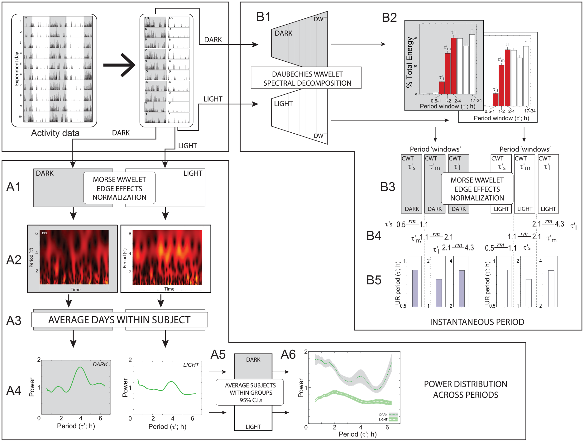
Ultradian power structure and ridge period analysis workflow. An example double-plotted locomotor activity record (actogram) of a mouse in a 12L:12D photocycle is depicted in the top panel, followed by schematic illustrations of two wavelet-based calculations for measurement of ultradian power and period. (A1-A6)
Normalization and Signal Averaging
Edge effects were managed by using a periodic boundary extension and removing 1.5 × the greatest period estimated (see Leise and Harrington, 2011; Leise, 2013) for justification and further discussion) (Figure 1A1). Scalograms were collated by treatment (photoperiod: 16 L:8D, 12 L:12D, 8 L:16D; sex: female, male; surgical treatment: ovariectomy (OVx), gonadectomy or orchiectomy (GDx), sham-OVx, and sham-GDx; duration of photoperiod treatment: 6 weeks, 8 weeks, and 10 weeks; circadian phase: light phase, dark phase) as appropriate for each experiment. The magnitude of each matrix was summed and divided by the total number of matrix cells, providing an average power for each activity record; each scalogram matrix was subsequently normalized by dividing by this average total power (Figure 1A1).
The complex magnitude of each matrix was then summed to a single cell and divided by the total number of matrix cells to compute an average total power from each individual time series record. Because photoperiod was manipulated in Experiment 3, this average was calculated for photoperiod for all groups based on the total number of cells in the 12 L:12D photoperiod; this permitted direct comparisons of magnitude across the different photoperiod treatment groups, by compensating for the different numbers of data bins in light and dark phase of different length. Next, to minimize individual differences in locomotor activity levels, the complex magnitude of each scalogram matrix was normalized by dividing by its average total power. Finally, to correct for edge distortion and to avoid biasing, the ends of each time series were extended periodically, and the resultant data were trimmed from either side of the scalogram matrix at 1.5 times the maximum value of the assessed period range (6.5 h), as recommended by Leise and Harrington (2011) (Figure 1A). The scalogram matrices (Figure 1A2) were averaged within each treatment group to compute a scalogram that best approximated the true matrix for the group (Figure 1A3). Comparable degrees of stationarity (or non-stationarity) were assumed for each grouping. Should such an assumption not be true, then the grouping of time series performed here may lead to changes in accuracy and/or precision in the measurements and possible downstream inferential errors, but in ways that we are not currently able to predict.
Variance Estimates and Group-Wise Differences
To facilitate comparisons of UR power distributions among treatment groups, each mouse’s normalized scalogram matrix was averaged across the time dimension into a power-period plot, which computes the average continuous wavelet transform power at each scale and its corresponding approximate ultradian period (designated as τ’ [tau-prime], to distinguish UR period [i.e., τ’] from CR period [τ]; Figure 1A4). These power-period plots were sorted and combined into average plots for each treatment group (Figure 1A5, 1A6). To generate measures of variability around the group mean, individual values of power distribution across period were grouped and bootstrapped 2000 times to calculate 95% confidence intervals (using the bootci function in MATLAB; Figure 1A5). Significant differences between groups were inferred to exist at UR periods where 95% CIs did not overlap. Example individual normalized scalograms are available in the supplementary methods.
Wavelet Ridge Extraction
Power (signal) exists at all frequencies, and the continuous wavelet transform analysis described above permitted evaluation of changes in the distribution of this power across all frequencies. We also determined whether experimental manipulations affected the ultradian frequencies at which maximal power occurred by utilizing wavelet ridge analyses to identify these values. In the continuous wavelet transform, the maximum wavelet ridge at each time point approximates the true frequency component, in this case the output of an ultradian clock[s] in the data, even in the presence of harmonic (e.g., circadian) circadian contamination. The wavelet ridge is defined as the maximum cross-correlation between time series and wavelet and approximates the instantaneous frequency (= 1/’τ) at every wavelet scale and time coordinate in the magnitude of the wavelet transform (Lilly and Olhede, 2010; Leise and Harrington, 2011; Leise, 2013, 2015).
The initial continuous wavelet transform window was characterized by a fragmented maximum wavelet ridge (e.g., scalogram in Figure 4B), indicating the presence of multiple ultradian components in the locomotor activity time series data. A discrete wavelet transform, described below, was used to apply multiple band pass filters and decompose locomotor activity time series data into a sum of wavelets or period bands (Figure 1B1). The detailed methodology along with validation of the windowing procedure are described in Experiment 1.2 and Figure 2. The results of the discrete wavelet transform analysis technique guided a re-windowing and reanalysis of the data. Locomotor activity time series for each subject were parsed by circadian phase (Figure 1B1) and again passed through the continuous wavelet transform with the analysis restricted to 1 of 3 period windows (Figure 1B3), corresponding to the 3 period bands of the discrete wavelet transform that contributed most to the UR waveform: a short UR period, from 53 h to 1.07 h [designated ‘tau-prime’ short, or τ’s]; a medium-duration period from 1.07 h to 2.13 h [τ’m]; and a longer period from 2.13 h to 4.26 h [τ’l] (Figure 1B2). Continuous wavelet transform analyses were computed separately for each period band and then normalized (Figure 1B3). Maximum wavelet power within each of these bands was used to characterize short, intermediate, and long-duration UR periods for each mouse (Figure 1B4, 1B5).
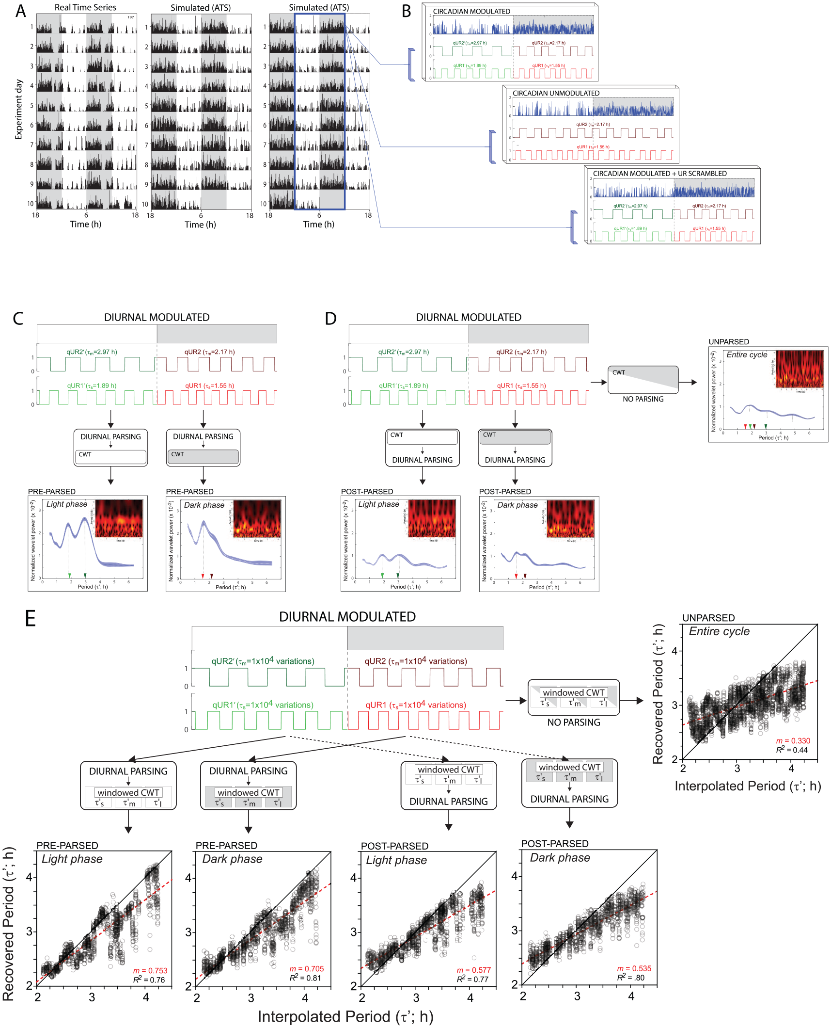
Validation of analyses using synthetic behavior containing known ultradian periods. (A) Representative double-plotted actograms depicting 10 days of locomotor activity (in a 12 L:12D photocycle, collected via passive infrared sensors) of a real C57BL6 J mouse (left), and in two synthetic actograms (simulated activity record; artificial time series; ATS) generated by a computational model of locomotor activity with known circadian and ultradian parameters. (B) Circadian locomotor activity records each contained randomly-selected UR periods in the τ’m and τ’l bands. In circadian modulated records, the period of each individual UR differed consistently between the light and the dark phases of the circadian cycle (top panel); in circadian unmodulated records, the period of each UR remained constant regardless of circadian phase (middle panel). Finally, in a control group, circadian-modulated URs were generated, but reordered randomly (‘scrambled’) within each circadian phase such that circadian structure and power were preserved, but all ultradian power was random across periods (bottom panel). (C, D)
Discrete Wavelet Transform and Data Detrending and Smoothing
To aid in interpreting the fragmented wavelet ridge observed, we adopted a technique recommended in the supplementary methods of Leise and Harrington (2011): the modified discrete wavelet transform was employed to decompose the time series to the 10th detail level into coefficients describing period between, 2
j
∆t → 2
j
+ 1∆t where j is the coefficient detail level and ∆t is the sampling interval. Edge effects were managed by extending end periodically and clipping 1.5 times the maximum period accessed (2048 minutes) which was clipped from each end. The energy contribution of each band was then quantified. Variance of the total time series can be described by the equation
Additional details of the wavelet analyses used in these experiments, including all simulations and validation steps appear in Experiments 1.1-1.3, and in Figures 1-3. Code files (MATLAB) used in analyses are available online (URLs in Data Availability Statement).
Additional Statistical Analyses
Lomb-Scargle periodogram power values (PN values) appeared non-normally distributed and were log10-transformed prior to analyses. Analysis of variance (ANOVA) was used to assess group differences and pairwise comparisons were evaluated with two-tailed t-tests when warranted by a significant F statistic. Note that locomotor activity data from 12 L:12D analyzed in Experiment 2 were also included in the ANOVA model for Experiment 4 to permit comparisons among all three photoperiods. Statistical analyses were performed using Statview v5 (SAS Institute) on a PC. Differences were considered significant if p ≤ 0.05.
Experiment 1. Validation of the Analytic Workflow
Because aspects of the data reduction and analyses are novel, we created a model of locomotor activity (see
Experiment 1.1: Validation of a Diurnal Parsing Procedure in the Presence and Absence of Circadian Modulation of the UR Waveform
Rationale
Because UR period, complexity and power may vary across the circadian cycle, evaluation of URs without regard for time-of-day may fail to capture important features of the UR waveform. To directly examine this circadian modulation, we analyzed diurnal activity data from the light and dark phases separately. Specifically, locomotor activity data generated during the part of the day when the room lights were on and when the room lights were off, were each extracted from the locomotor activity record time series, and were concatenated into separate ‘parsed’ records consisting of light-phase only or dark-phase only data. These parsed records were then evaluated via the continuous wavelet transform and/or discrete wavelet transform as described in Figures 1 and 2. The simulations conducted in Experiment 1.1 evaluated: (1) the accuracy and precision of this procedure by comparing its handling of parsed vs non-parsed data, and (2) the effect of performing the diurnal parsing prior to versus after the wavelet transform was performed. In order to ensure that the diurnal splicing procedure itself did not generate systematic differences in UR period or power, we assessed the precision of the procedure by evaluating simulated activity data, generated in silico, which contained URs with defined ultradian periods and which varied in period between the light and dark phases (circadian modulated URs) or remained at a fixed period over the circadian cycle (circadian unmodulated URs).
Locomotor activity model and simulation data
A model comprised of 10 days of locomotor activity was created to mimic actual mouse activity data in amplitude and variance (except for aspects that were experimentally manipulated as described below; Figure 2A). The locomotor activity model was set to have a robust CR with a period of 24 h, either 2 or 4 URs with known periods, and a variable but reasonable amount of background noise. URs were randomly selected, with the condition that records were always generated with both ‘long’ (2.13-4.26 h) and ‘medium’ (1.07-2.13 h) URs. For full details of the mathematical operations used to generate locomotor activity by this model, see Supplementary Material: Locomotor Activity Model and Simulation Data .
The model was then used to generate three treatment groups (n = 10 simulated subjects / group; Figure 2A). In one experimental group (‘CR modulated’), UR period was modulated by circadian phase: long- and intermediate-period URs inserted into the light phase time series had different periods than the long- and intermediate-period URs that were interpolated into the dark phase of the time series (Figure 2B). In a second group (‘CR unmodulated’), URs were not modulated by circadian phase: within each locomotor activity record, identical long- and intermediate-period URs were interpolated into both the light and dark phases (Figure 2B). Importantly, the modulated and unmodulated groups were generated at the same time using the same dark phase URs, so that the only differences between them was in the period of the light phase URs. Finally, a control group (‘no UR’), was created by taking the 10 modulated versions of the artificial activity records and scrambling the data within each “day” and “night” (i.e., light and dark phases, respectively) such that the circadian structure was preserved but all ultradian structure was randomly shuffled (Figure 2B). To complete the simulation, the creation of the three UR treatment groups (CR modulated, CR unmodulated, or no UR; n = 10 records / group) was performed 100 times with different, random-selected long- and intermediate-duration URs. Using these datasets, we then performed the quantitative analyses of UR period and power (as outlined in Figure 1) for each of the 1000 total simulations.
In performing these analyses, we also evaluated whether the analysis stage at which the diurnal parsing procedure was performed affected the accuracy and precision of the resulting power and period measurements. Thus, the diurnal parsing procedure (concatenation into light-phase only and dark-phase only records) was performed: (1) before the data were analyzed by the continuous wavelet transform (Figure 2C), (2) after the data were analyzed by the continuous wavelet transform (Figure 2D), or (3) not at all (i.e., the data remained unparsed at all stages of analysis; Figure 2D). Following the wavelet transform, all matrices were normalized, with their edges trimmed before collapsing across time (experimental days) to generate two-dimensional period-power plots, which permitted evaluation of the effects of modulation and parsing on the accuracy and precision of the continuous wavelet transform analysis. Simulations were performed across a range of β’ values (4-12) and results remained stable although, as expected, higher β’ values improved frequency resolution.
Experiment 1.2: Segmentation of the Ultradian Frequency Spectrum
Rationale
URs do not resonate with any known geophysical periodicity, thus there is no a priori expectation that UR power should occur at a single period (cf. CRs). Specification of just a single UR period, therefore, likely fails to capture the polyrhythmic nature of URs. Indeed, individuals exhibit URs in multiple traits, which may manifest as power at multiple periodicities. Accurate characterization of the UR spectrum should capture this waveform complexity. Wavelet transforms are well-suited for quantifying UR power simultaneously at multiple periodicities: peak ridge power in the continuous wavelet transform matrix approximates the instantaneous period of the UR (Lilly and Olhede, 2010; Leise and Harrington, 2011; Lilly and Olhede, 2012; Leise, 2013, 2015), but at many times of day, peak scalogram power may occur at multiple periodicities (Figure 1A; Figure 4B and 4C). Segmenting these fragmented scalograms into multiple period bands would permit quantification of peak UR periods therein. Simply identifying the few highest peaks in the scalogram is inadequate in this regard, as it introduces biases due to clustered peaks and difficulties distinguishing among multiple peaks within a cluster. Ideally, segmentation of the UR domain should not be arbitrary (e.g., period bands of 2 h, or a similarly convenient integer), but rather should be objectively driven, informed by the actual distribution of where power lies in the ultradian domain. The wavelet ridge extraction (described above) offers a suitable method for objective segmentation of the ultradian domain into period ‘bands’.
Quantitative procedures and workflow
Locomotor activity time series were decomposed with the modified discrete wavelet transform (discrete wavelet transform) from the 1st to the 10th detail of the discrete wavelet transform (defined by 2
j
∆t → 2
j
+ 1 ∆t, where j is the detail level and ∆t is the sampling interval). This resulted in the generation of period bands (termed ‘details’ in the discrete wavelet transform) ranging from 2 to 4 min through 17-34 h; the latter of which contained the fundamental circadian component (see Methods: Wavelet ridge extraction). Spectral decomposition was performed using a symlet wavelet (also termed a Daubechies least asymmetric wavelet) with 6 vanishing moments (Figure 1B1), following procedures and considerations for this analysis as it applies to behavioral time series data described in detail in Leise and Harrington (2011). In order to impartially characterize the relative contribution of each detail—and thus generate an unbiased estimate of the relative importance of each detail to the overall rhythmic structure of the locomotor activity waveform—we calculated the energy (i.e., variance) explained by each normalized wavelet detail energy as described in
Data
First, in order to specify the distribution of rhythmic power in vivo, we used locomotor activity records (10 days, 1 min bins) obtained from male (n = 20) and female (n = 20) mice housed in 12 L:12D. For the initial discrete wavelet transform symlet analysis, locomotor activity data contained only endogenously-generated URs (i.e., simulated URs were not added; Figure 1B1-1B2). The resulting power distribution clearly identified three detail bands which explained a substantial proportion of the variance in spectral power (a short UR period, from .53 h to 1.07 h [designated ‘tau-prime’ short, or τ’s]; a medium-duration period from 1.07 h to 2.13 h [τ’m]; and a longer period from 2.13 h to 4.26 h [τ’l]; Figure 1B4). These bands were used thereafter to objectively segment the ultradian domain and specify UR periods using continuous wavelet transform (Figure 1B3-1B5).
Next, simulation data from Experiment 1, comprised of locomotor activity records created with circadian-modulated (n = 2000) and -unmodulated (n = 2000) UR periods (cf. Figure 2A and 2B) were again passed through the continuous wavelet transform, with each analysis limited to 2 of the 3 period windows specified above (τ’m and τ’l, which corresponded to the UR periods with which the simulated data were created). Each continuous wavelet transform analysis computed the maximum ridge value, the mean scale, and the period corresponding to that scale value for each individual record. Continuous wavelet transform analyses were computed separately for each period band as in Figure 1B3-1B5, and normalized. The period at which scalogram matrix cross-correlational power was maximal was used to define the instantaneous period in a given τ-band. Linear regression analyses were calculated to evaluate the accuracy and precision of the wavelet ridge procedure in recovering interpolated UR values.
Experiment 1.3: In Vivo Validity
Rationale
This experiment sought to determine whether the wavelet workflow described above was capable of detecting and adequately characterizing rhythmic power not merely in period-recovery simulations, but in locomotor activity data generated by actual mice. In order to possess in vivo validity, the wavelet workflow should be capable of quantifying functionally significant overt behavior.
CRs in vertebrate physiology and behavior are generated by transcriptional-translational feedback loops of circadian clock genes and their protein products. One element of this feedback loop, Period 2 (and its protein product, PER2) is critical for the integrity of the organismal circadian network: germline mutant mice with a functional deletion of the mPER2 protein dimerization PAS domain (mPer2 Brdm1 ; Per2m/m mice) entrain to 24 h L:D cycles, but upon transfer to constant darkness exhibit an extremely short free-running circadian period (~22-23 h), and subsequently become behaviorally circadian arrhythmic (Zheng et al., 1999). Moreover, Per2 m/m mice have been characterized as exhibiting robust increases in UR power after the loss of circadian rhythmicity in constant darkness (Zheng et al., 1999; Bae et al., 2001; Zheng et al., 2001; Abe et al., 2002; Riggle et al., 2022). We used Per2 m/m mice to evaluate the ability of the continuous wavelet transform analysis described above to detect: (1) changes in circadian period upon transfer from long day to constant darkness, (2) the loss of circadian rhythmicity following prolonged exposure to constant darkness, and (3) the emergence of power in the ultradian domain following the loss of CRs, and in doing so further characterize the ecological validity of the analytic workflow used here.
Animals and data collection
This experiment used mutant (Per2m/m: B6. Cg-Per2tm1Brd Tyrc-Brd/J, JAX#: 003819 [albino]) and WT (C57BL/6J, JAX#: 000664 [black]) mice ordered directly from the Jackson Laboratories (Bar Harbor, ME, USA). Female mice (Per2m/m: n = 5; WT: n = 7; ~5 weeks of age) were singly housed in 12L:12D under passive infrared motion sensors. A more extensive analysis of data from these mice has been reported elsewhere (Riggle et al., 2022). The data described here (in Experiment 1.3) are a re-analysis of locomotor activity records from Per2m/m mice that were previously reported in a study of sex differences in circadian behavior (Riggle et al., 2022); the data are used here solely for the purposes of validating the accuracy and precision of the continuous wavelet transform’s ability to measure period and power in a model of circadian arrhythmia. Mice were kept in 12L:12D to establish a baseline of entrained locomotor activity and were then transferred to constant darkness (DD). Locomotor activity data were analyzed using the continuous wavelet transform analytic pipeline described in Experiment 1.1 and illustrated in Figure 1A and 1B. Specifically, (1) locomotor activity records were diurnally parsed, and light-phase and dark-phase data were concatenated and subjected to the continuous wavelet transform to generate scalograms and power distribution plots (Figure 1A), and (2) diurnally parsed data were band-pass filtered into short-, intermediate- and long-duration τ’ windows and subjected to the continuous wavelet transform to identify peak instantaneous UR period within each window (Figure 1A).
Experiment 2. Circadian and Sex Differences in UR Period and Power
Methods
Male (n = 20) and female (n = 20) mice (4 weeks of age) were singly housed in 12 L:12D upon arrival in the laboratory. Following < 1 week of adaptation, passive infrared motion detectors were mounted above the cages and home cage locomotor activity data collection began (= week 0). Locomotor activity during the 10 days immediately preceding the end of week 6 (on day 42 of the study) were exported as a time series for behavioral analyses via the continuous wavelet transform analytic workflows described and validated in Experiment 1.
In addition, in an effort to replicate the week 6 data and to evaluate the stability and precision of quantitative measures of UR parameters generated by the continuous wavelet transform, identical continuous wavelet transform measures were repeated on the same mice 2 weeks later (beginning on week 8). Due to loss of data from channel dropouts, final sample sizes were as follows: week 6; 18 females and 17 males; week 8: 18 females and 16 males. After the week 8-10 measurement interval, photoperiod manipulations began (Experiment 3).
Experiment 3. Effects of Circadian Entrainment to Long and Short Photoperiods on URs
Methods
Following 10 weeks of exposure to 12 L:12D in Experiment 2, male (n = 20) and female (n = 20) mice were subjected to a sequence of increasing and decreasing day lengths as follows: mice were transferred from 12 L:12D (intermediate day; IntD) to 16 L:8D (long days; LD), where they remained for 6 weeks; mice then were transferred to 8 L:16D (short days; SD), where they remained for 10 weeks. As in previous analyses, 10 days of locomotor activity data were collected and analyzed via continuous wavelet transform. In long days and short days, locomotor activity was examined after 6 weeks and in short days replicated again twice over 4 additional weeks. Final sample size in each condition was as follows: long day (week 6: 19 F and 19 M), short day (20 F and 20 M).
Experiment 4. Effects of Gonadectomy on URs
Methods
A separate cohort of 4-week-old male and female mice, ordered from Jackson Labs, were subjected to surgical gonadectomy (males: orchidectomy [GDx, n = 17]; females: ovariectomy [OVx; n = 7]) or were sham-operated (sham-GDx [n = 15]; sham-OVx [n = 7]). Gonadectomy was performed under 3%-4% isoflurane/O2 gas anesthesia. In males, a ventral midline incision was made, testicular blood vessels were ligated and cauterized, and testes removed. In females, after a dorsal midline incision, ovarian blood vessels were ligated and cauterized, and the ovaries were removed. Incisions were closed with non-resorbable vinyl sutures and cutaneous wound clips. Topical antibiotic ointment was applied to the wound site. Analgesic buprenorphine was administered immediately after surgery and every 12 h for the next 48 h. The sham procedure replicated the GDx or OVx procedure, except tissues were not ligated or removed. Animals were allowed 7 weeks to recover, after which time locomotor activity data were collected for 4 weeks via home-cage passive infrared motion detectors. Surgical condition was confirmed in all mice at the end of the study via necropsy.
Results
Experiment 1.1: Validation of the Analytic Workflow—Circadian Modulation and Parsing
In order to validate the analytic workflow (Figure 1), simulated locomotor activity records were created so as to contain a naturalistic waveform of circadian activity interpolated with known ultradian periods (τ’) (see Figure 2A for representative records; see supplementary methods for details of activity simulation). Each record contained a medium-duration (τ’m) and a longer-duration (τ’l) UR, the periods of which either remained fixed over the entire circadian cycle (unmodulated), or varied systematically between circadian phases (modulated; Figure 2B). Light phase and dark phase activity were separated (parsed) for ultradian power structure and ridge period analyses either prior to (‘pre-parsed’) or after (post-parsed’) performing each wavelet analysis. In pre-parsed records, ultradian power structure plots contained clear, high-amplitude peaks in scalogram power that corresponded closely to the interpolated τ’m and τ’l, and differed between the light and dark phases (i.e., were circadian-modulated; Figure 2C). In contrast, when the same activity records were either parsed after the analyses (post-parsed) or not parsed at all (unparsed), power structure waveforms were distorted: UR spectral power was reduced, peaks appeared less distinct, and they occurred at values that did not as closely match the interpolated URs (Figure 2D). Diurnal parsing after performing the analyses also created sharp crepuscular discontinuities (edges) in the wavelet matrix, readily visualized by comparing post-parsed and pre-parsed scalograms (inset plots in Figure 2C and 2D). These near-instantaneous shifts in power are unlikely to reflect actual changes in URs over time in vivo as daily activity onsets and offsets are not generally discrete transitions when measured with passive infrared detectors. Finally, power structure analyses of unparsed data also yielded multiple peaks that approximated the interpolated UR periods; however, outside of an in silico period-recovery paradigm, it would not be possible to determine which phase of the circadian cycle each individual UR was occurring in.
Experiment 1.2: Segmentation of the Ultradian Frequency Spectrum
A spectral decomposition analysis using a discrete wavelet transform identified 3 period bands (τ’ bands) that contained a disproportionate amount of the total variance in the ultradian domain: (1) a short UR band, from 0.53 h to 1.07 h [designated ‘tau-prime short’, or τ’s]; (2) an intermediate-duration UR band, from 1.07 h to 2.13 h [τ’m]; and (3) a longer UR band, from 2.13 h to 4.26 h [τ’l] (see Figure 4F). Note that the circadian period band (discrete wavelet transform detail i = 10) also contained a substantial portion of the spectral variance. In addition, these three bands (which contain periods from 0.53 h to 4.26 h; discrete wavelet transform details 5-7), exclude information from power at periods of 8 h and 12 h, and thereby avoid artifacts arising from the interval between light-dark transitions in long (16 L:8D), intermediate (12 L:12D), and short (8:16D) photoperiods.
Instantaneous period in each of these three τ’-bands was measured in activity records from Experiment 1.1, and a period-recovery analysis was performed to evaluate accuracy and precision of the period estimates. Simulated locomotor activity time series data, generated with modulated or unmodulated URs, were passed through the continuous wavelet transform limited to either the τ’m or the τ’l band. As in Experiment. 1.1, data were either pre-parsed or post-parsed. Peak scalogram power defined instantaneous UR period for a given τ’-band. Period-recovery analyses indicated that measures of instantaneous period in pre-parsed records were strongly and positively correlated with the periods of interpolated URs (regression coefficients: light phase = 0.753; dark phase = 0.705; p < 0.0001; Figure 2E). Post-parsing yielded substantially lower regression coefficients (light phase = 0.577; dark phase = 0.535; p < 0.0001; Figure 2E; Table S1).
In sum, simulation results from Experiments 1.1 and 1.2 indicate that power structure and ridge period calculations reliably recover the expected UR power and period values from a complex artificial activity waveform. Post-parsed and pre-parsed data yielded UR peaks with period and phase accuracy, although peaks generated by pre-parsed data were generally higher in amplitude and thus more precise. Post-parsed data also exhibited sharp crepuscular discontinuities in the wavelet matrix, which are unlikely to correspond to actual activity and thus may constitute artifacts. Period measures in the decomposed τ’m and τ’l bands were also more accurate when locomotor activity records were pre-parsed. Taken together, the simulation data indicate that power structure and ridge period calculations: (1) accurately quantify the distribution of rhythmic power in complex (non-stationary, multiple periods) ultradian activity records, (2) permit specification of UR power and period features to specific circadian phases via parsing, and (3) yield more accurate and precise results when parsing is performed prior to wavelet analyses. It is noteworthy, however, that there is some underestimation of periods at the edge of the chosen analysis windows. This may be due to spectral leakage. Depending on experimental question it may be useful to apply more specific windows to periods measured at the edge of analysis windows.
Experiment 1.3: In Vivo Validation
Among WT mice housed in 12 L:12D, power structure analyses identified a clear circadian period at 24 h (Figure 3A). Following transfer to constant darkness, power in the circadian domain remained ~24 h in WT mice (Figure 3A) but exhibited a period of ~22-23 h in Per2m/m mice (see Methods for more details), as previously reported (Figure 3B; Zheng et al., 1999; Riggle et al., 2022). Subsequently, 4 of 5 Per2 m/m mice exhibited circadian arrhythmicity in constant darkness; this was accompanied by a broad spectrum reduction in power in the circadian waveform (Figure 3B). An increase in UR power (~2-6 h; Figure 3B) was commonly associated with circadian arrhythmia, an observation consistent with prior reports of disinhibition of URs in arrhythmic mutant mice (Zheng et al., 1999; Bunger et al., 2000; Zheng et al., 2001). In contrast, WT mice retained CRs in constant darkness and exhibited no obvious changes in CR or UR power as compared to their measures during early exposure to constant darkness (Figure 3A). Finally, ridge period analyses were performed on locomotor activity sampled from intervals during which distinct chronotypes (free-run, arrhythmicity). τ’l values were calculated for each mouse and aggregated within genotype groups: τ’l was similar in WT and Per2m/m mice while free-running in constant darkness, but was significantly longer in Per2m/m mice after they became circadian arrhythmic (Figure 3C).
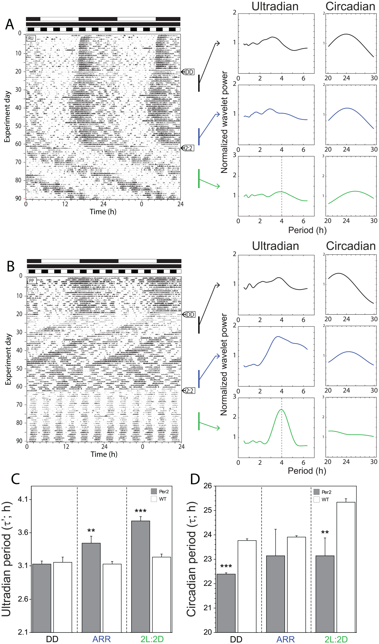
Validation of analyses using real behavior driven with a known ultradian period. Representative double-plotted actograms of (A) a WT female mouse and (B) a homozygous Per2Bdrm1 mutant (Per2m/m) female mouse housed in a 12L:12D light cycle, then in constant darkness (indicated by ➜ “DD”), and finally in a 2L:2D light:dark cycle (indicated by ➜ “2:2”). Black and white bars along the abscissae indicate intervals of darkness and light, respectively. Black (early DD, when wildtype and Per2 m/m were both free running), blue (late DD when Per2m/m mice were arrhythmic (ARR) and wildtype mice remained free running), and green (during exposure to 2L:2D) vertical bars indicate 10-day intervals of locomotor activity that were subjected to wavelet analyses, the results of which appear to the right of each corresponding interval. Separate power plots depict ultradian (0.5-6.5 h) and circadian (20-30 h) analysis windows for each of the analyzed epochs. Continuous wavelet transform and power-period plots were calculated as described in Figure 1A. (C, D) Mean +/- SEM (standard error of mean) ultradian (τ’l band) and circadian (20-30 h band) period of female WT mice (n = 7) and Per2m/m mice that exhibited circadian arrhythmia in constant darkness (n = 4). UR periods (maximum wavelet ridge values) were calculated as described in Figure 1B. **p < 0.01. ***p < 0.001 vs WT value. Abbreviations: WT = wild-type; DD = constant darkness; ARR = arrhythmic.
Mice were then exposed to a high-frequency T-cycle (photocycle) (2 L:2D; period = 4 h) for several weeks. WT mice continued to exhibit free-running locomotor activity in 2 L:2D, with a period > 24 h, with some evidence of masking effects imposed by the T-cycle (Figure 3A). Per2m/m mice, in contrast, exhibited strong masking responses to 2L:2D, with high levels of locomotor activity and rest aligned with the dark and light phases, respectively. Thus, Per2m/m mice manifested a behavioral UR with a known periodicity, driven by the T-cycle. We then evaluated whether power structure and ridge period analyses could accurately quantify this environmentally-driven behavioral UR. Power structure plots of Per2m/m mice contained clear and prominent maxima at periods approximating 4 h, and ridge period measures in the τ’l band also indicated that activity occurred with a period near 4 h (mean +/- SEM = 3.77 +/-0.07).
In summary, Experiment 1 provided convergent evidence validating the accuracy and precision of wavelet-based analyses for the measurement of ultradian power distribution and period in mice. We next sought to extend these analyses to evaluate URs in mice exposed to environmental and hormonal manipulations previously reported to modulate the UR waveform in diverse mammalian models. Thus, Experiments 2-4 employed power structure and ridge period analyses to quantify group-level effects of sex (Experiment 2), circadian entrainment (Experiment 3), and gonadectomy (Experiment 4) on UR power and period.
Experiment 2. Circadian and Sex Differences in UR Period and Power
Circadian Rhythms
Male (n = 20) and female (n = 20) mice housed in 12 L:12D exhibited normal nocturnal CRs in locomotor activity, with intermittent active bouts during the light phase (Figure 4A). After the exclusion of broken channels, the Lomb-Scargle periodogram identified the presence of 24 h rhythm in all individuals, indicative of entrainment to the photocycle. Circadian power was greater in females than males (Suppl. Fig. S1 F1,33 = 4.55, p < 0.05; cf. Iwahana et al., 2008; Yan and Silver, 2016).
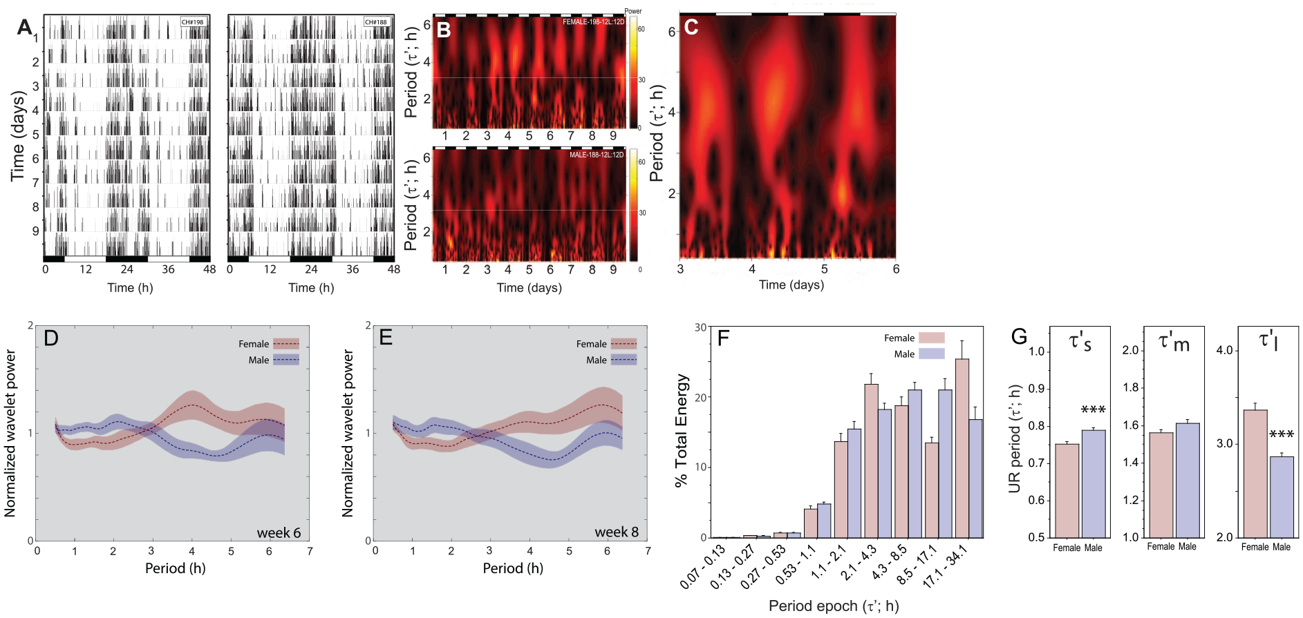
Sex differences in ultradian power and period. (A) Representative double-plotted locomotor activity records of female (left) and male (right) C57BL6/J mice housed in a 12 L:12D photocycle over 10 days as measured with passive infrared recording devices in the home cage. Black and white bars along the abscissae indicate intervals of darkness and light, respectively. (B) Scalograms depicting the scaled cross-correlation value of the Morse wavelet (continuous wavelet transform; β = 10; γ = 3; UR analysis window: 0.5-6.5 h) for the 10-day time series of locomotor activity in panel A. Magnitude scale bar references panels B &C. (C) Re-depiction of 72 h from the scalogram in panel B permits visualization of relatively higher cross-correlations (i.e., power) present at multiple ultradian periods simultaneously. (D) Average cross-correlational power at each scale-approximated period derived from the continuous wavelet transform on a time series consisting of locomotor activity during 10 consecutive dark phases in 12 L:12D (pre-parsed records). Separate power curves are depicted for male (blue) and female (red) mice; the curves depict mean ± 95% confidence intervals (CIs) generated by bootstrapping male and female groupings of these curves (bootstrapped: 2000x; 18 females and 17 males). (E) Power/period curve generated by continuous wavelet transform of 10 days of dark phase locomotor activity data as in panel D from the same mice as depicted in panel D, 2 weeks later (i.e., on week 8 in 12 L:12D; 18 females and 16 males). (F) Mean + SEM percent of total spectral energy explained by each detail level of wavelet coefficients for the time series consisting of locomotor activity over 10 consecutive days in 12 L:12D of female and male mice. Abscissa indicates period of details 2-10 (in h). Details 5, 6 and 7 encompass intervals defined as short, medium and long UR periods (τ’s, τ’m, τ’l, respectively). (G) Mean (+ SEM) ultradian periods (τ’) of pre-parsed dark phase locomotor activity data within each of the 3 UR analysis intervals identified in panel F (short τ’[τ’s: 0.53-1.1 h], medium τ’ [τ’m: 1.1-2.1 h], and long τ’ [τ’l: 2.1-4.3 h]), and via continuous wavelet transform methods described in Figure 1B. ***p < 0.001 vs. corresponding female value. Abbreviation: UR = ultradian rhythms.
Ultradian Rhythms
URs were next evaluated using power and period analyses described in Figure 1 and validated in Experiments 1.1 to 1.3 (see Supplementary Data for example individual scalograms). Locomotor activity (10 days) were pre-parsed into dark phase and light phase records prior to all analyses.
UR power distribution
Scalograms identified multiple regions of high cross-correlation in the ultradian band (Figure 4B); diurnal variations in UR power and period were also common (Figure 4C). During the dark phase, power structure plots revealed a non-uniform power distribution across the ultradian spectrum for both sexes. In females, power peaked at ~4.0 h and was lower across a range of shorter periods (τ’: 1.0 to 3.5 h; Figure 4D). In males, power was highest in a similar range of shorter periods (τ’: ~1.0 to 3.0 h) with a conspicuous decrease in the ~4.0 h range (male (n = 18) and female n = 17); Figure 4D). Sex differences in the distribution of rhythmic power were identified via non-overlapping 95% CIs: power was greater in males from ~0.75 h to ~2.25 h and in females from ~3 h to ~5 h. power structure analyses performed 2 weeks later (week 8 in 12 L:12D) yielded strikingly similar results (Figure 4E), indicating that power distribution across ultradian periods is relatively stable and reliable over time, within and between sexes.
During the light phase, power structure plots were similar in males and females (Suppl. Fig. S2A). Power peaked at ~3.0 h, with lower power values preceding and following the peak. Light phase period-power relations were also similar on weeks 6 and 8 (Suppl. Fig. S2B).
UR period
Fragmented wavelet scalograms were decomposed using a symlet wavelet (as described in Experiment 1.2) to identify the distribution of spectral energy across the UR domain. Males and females both exhibited substantial power in the τ’s, τ’m, and τ’l bands (encompassing 0.53 to 1.07 h, 1.07 to 2.13 h, and 2.13 h to 4.26 h; Figure 4F). As in Experiment 1 these bands were analyzed individually by extrapolating UR period from the maximum value of the continuous wavelet transform scalogram within each band. τ’l was significantly longer in females than males in the dark phase (Figure 4G; p < 0.0001), but not in the light (Suppl. Fig. S2 C; p > 0.30; sex x phase interaction: F1,66 = 21.7, p < 0.0001); small but significant sex differences were also evident in dark phase τ’s (p < 0.005; Figure 4 G). Light phase UR period did not differ between males and females in any period band (p > 0.30, all comparisons). Overall, UR period was significantly longer during the light phase compared to the dark phase in the τ’s band (F1,66 = 178.4, p < 0.0001) and in the τ’m band (F1,66 = 15.0, p < 0.0005), and among males in the τ’l band (p < 0.05) (Figure 4G vs Suppl. Fig. S2 C).
Period measures obtained 2 weeks later yielded similar, phase-specific effects of sex on τ’l (sex x phase interaction: F1,64 = 29.0, p < 0.0001), τ’s (p < 0.005), and no evidence of sex differences in light phase UR period (p > 0.05, all τ’ bands). Period measures from week 6 also positively correlated with those obtained 2 weeks later (week 8: τ’s slope = 0.82, p < 0.0001; τ’m slope = 0.45, p < 0.0005; τ’l slope = 0.73, p < 0.0001), indicating reliability and stability over time.
In sum, dark phase UR power was distributed across shorter periods in males compared to females, but light phase power was distributed similarly in both sexes. During the active phase τ’s was longer in males, and τ’l was longer in females. Overall, UR periods were also longer in the rest (light) phase. Taken together, power structure and ridge period analyses exhibited a precision sufficient to identify multiple sex differences in UR power and period which confirm and extend prior studies of sex differences in ultradian behavior patterns (Wollnik and Dohler, 1986; Prendergast et al., 2012b; Prendergast and Zucker, 2016; Smarr et al., 2017).
Experiment 3. Effects of Circadian Entrainment to Long and Short Photoperiods on URs
We next examined whether the entrainment state of the circadian pacemaker modulates URs by exposing all mice to a series of different experimental day lengths: intermediate- (12 L:12D), long- (16 L:8D) and short-duration (8 L:16D) photoperiods. Lomb-Scargle periodogram analyses first confirmed that mice exhibited typical nocturnal patterns of circadian entrainment to the respective experimental photoperiods (Suppl. Figs. S1A-S1 F). Peak values in the periodogram were greater in females than males (F1.107 = 24.3; p < 0.0001; Suppl. Fig. S1G). CR power was comparable in all photoperiods among females (p > 0.30, all comparisons), but among males, power was greater in long days than short days (p < 0.05; Suppl. Fig. S1G).
UR Power Distribution
Entrainment to long and short photocycles systematically altered UR power in both females and males (Figure 5A and 5B). In the dark phase, overall UR power was greater in long days than in intermediate days, and greater in intermediate days compared to short days; sex differences in the distribution of UR power were maintained in all photoperiods (Figure 5C-5E). Photoperiod also conspicuously reshaped power structure waveforms. In long days, power was concentrated at ~4 h in both sexes, whereas in short days peak UR power shifted to higher (> 5 h) periods. In all photocycles, males exhibited greater high-frequency UR power (τ’< 2 h) than females. Conversely, light phase UR power was greatest in short days, and decreased monotonically with longer day lengths (Suppl. Fig. S3A-S3C). In short days, light phase power also shifted toward shorter periods (1-3 h) and away from longer periods (Suppl. Fig. S3C). Regardless of day length, however, females and males exhibited remarkably similar distributions of light phase UR power (Suppl. Fig. S3).
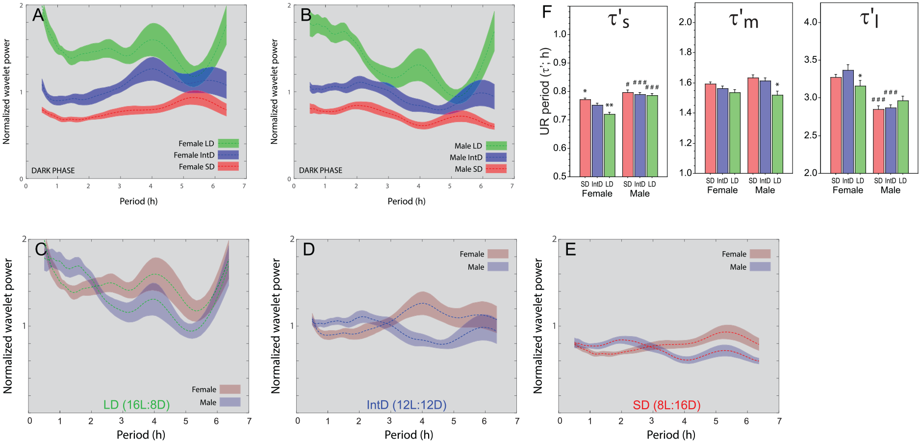
Photoperiodic modulation of ultradian power and period. Power-period plots (± 95% CI) calculated by continuous wavelet transform of 10 days of pre-parsed dark phase locomotor activity data from (A) female (long day: n = 19, intermediate day: n = 18, short day: n = 20) and (B) male (long day: n = 19, intermediate day: n = 17, short day: n = 20) mice after adaptation to 16 L:8D (green), 12 L:12D (blue) or 8 L:16D (red) photoperiods. See Figure S1 for confirmation of circadian entrainment. (C-E) Re-depiction of dark phase power/ period curves from panels A and B to permit direct comparisons of male and female mice in (C) 16 L:8D, (D) 12 L:12D, and (E) 8 L:16D. (F) Mean (± SEM) instantaneous ultradian periods (τ’) of pre-parsed dark phase locomotor activity data in the τ’s, τ’m and τ’l period analysis bands.:*p < 0.05, **p < 0.01 ***p < 0.001 vs IntD value within sex; #p < 0.05, ###p < 0.001 vs females within DL. Abbreviations: CI = confidence interval; UR = ultradian rhythms.
UR Period
UR period depended on the interaction of photoperiod and sex, in a circadian phase-specific manner (τ’s: F2,214 = 3.97, p < 0.05; τ’m: F2,214 = 3.18, p < 0.05; τ’l: F2,214 = 3.58, p < 0.05; Figure 5F). In the dark phase τ’s of females lengthened as day length decreased (p < 0.05, all comparisons), but male τ’s did not (p > 0.30, all comparisons); τ’m was shortest in long days in both sexes (p < 0.05 vs short day values, both comparisons; Figure 5F). Photoperiod was largely without effect on τ’l. Finally, in most instances, τ’s was longer in males and τ’l was longer in females (Figure 5F). In the light phase, sex differences were largely absent across most photoperiods and τ’ bands (Suppl. Fig. S3D).
Longitudinal evaluation in short days
Power structure of dark phase URs on week 6 was similar to that on weeks 8 and 10 (Suppl. Fig. S4 C-S4D), and a similar pattern of results obtained for light phase locomotor activity data, with the exception of an increase in longer-period (~5-6 h) power on week 10 in both sexes (Suppl. Fig. S4). Similarly, there was no main effect of week in short days (F2,228 = 2.2, p > 0.10, all ANOVAs) and no interaction effect of week x sex x phase (F2,228 = 52, p > 0.50, all ANOVAs) on UR period in any of the 3 period bands.
Diurnal rhythms in UR power
Direct juxtaposition of dark and light phase period-power plots identified striking diurnal modulation of power structure distributions (Suppl. Fig. S5). In long days, dark phase power exceeded light phase power across the entire UR period domain (Suppl. Fig. S5A), this diurnal modulation of UR power was greatly attenuated in intermediate days (Suppl. Fig. S5B, E), and reversed in short days (Suppl. Fig. S5 C, F).
In sum, day length affected ultradian period and power, and exerted opposite effects in the dark and light phases. In both sexes, the incremental decrease in day length attenuated dark phase UR power and augmented light phase UR power. Together, power structure and ridge period analyses identified consistent patterns of power and period modulation by photoperiod in male and female mice.
Experiment 4: Effects of Gonadectomy on URs
This experiment tested the hypothesis that sex differences in UR power and period are maintained by concurrent gonadal hormone secretion (i.e., activational effects).
UR Power Distribution
As in Experiment 2, gonad-intact females exhibited lower dark phase UR power than intact males across a range of shorter (1.5-3 h) periods (Figure 6A), but power in the 3-5 h range was not significantly greater than that of males (cf. Figure 4D). OVx caused minor increases and decreases in dark phase UR power, in narrow bands around 2 and 4 h, respectively (Figure 6B), and GDx increased power between 0.5 and 1 h and decreased power from 2.5 to 3.5 h (Figure 6C). Light phase power again peaked between 3-4 h and was largely comparable in females and males, (Figure 6E; cf. Suppl. Fig. S2). OVx did not affect light phase UR power (Figure 6F), but GDx flattened the power distribution: increasing power in periods < 2 h and decreasing power in periods > 2.5 h (Figure 6 G).
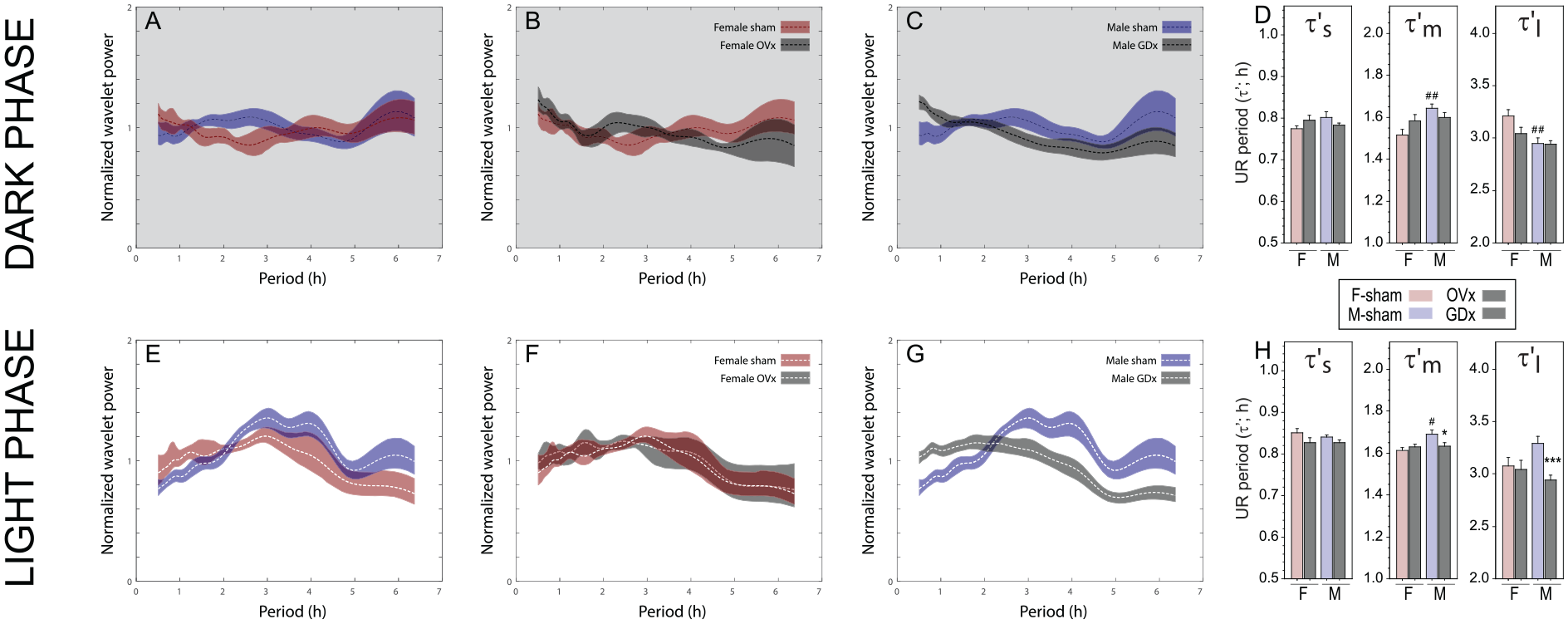
Effects of gonadal hormones on ultradian power and period. Power-period plots (± 95% CI) calculated by continuous wavelet transform of 10 days of pre-parsed dark phase (top row) and light phase (bottom row) locomotor activity records from (A, E) sham-operated female (n = 7) and male (n = 15) mice, (B, F) ovariectomized (OVx; n = 7)) and sham-operated (n = 7) female mice, and (C, G) orchidectomized (GDx; n = 17) and sham-operated (n = 15) male mice. (D, H) Mean (± SEM) instantaneous ultradian periods (τ’) of pre-parsed dark phase (panel D) and light phase (panel H) locomotor activity data in the τ’s, τ’m and τ’l period analysis bands. *p < 0.05, ***p < 0.001 vs sham-value within sex; #p < 0.05, ##p < 0.01 vs females, within surgical condition. Abbreviations: CI = confidence interval; UR = ultradian rhythms.
UR Period
As in Experiment 2, τ’l depended on sex in a phase-specific manner, and this relation depended on gonadal status (sex x surgery x phase interaction: F1,84 = 7.10, p < 0.001; Figure 6D and 6 H). Neither dark phase nor light phase τ’l was affected by OVx (p > 0.50, both comparisons), but GDx caused a decrease in light phase τ’l of ~ 20 min (p < 0.0005) without affecting dark phase τ’l (p > 0.80). Sex and gonadal condition also interacted to affect τ’m (F1,84 = 7.80, p < 0.01): GDx caused a small but significant decrease in light phase τ’m (p < 0.05; Figure 6 H).
Effects of sex on UR period among intact mice in Experiment 4 were similar to those obtained in Experiment 2, despite a smaller female sample size. Specifically, the effect of sex on τ’l depended on circadian phase (sex x phase interaction: F = 1,40 = 12.0, p < 0.005). In addition, light phase period was greater than dark phase period in the τ’s (F1,40 = 24.3, p < 0.0001) and τ’m (F1,40 = 9.73, p < 0.005) bands, and among males (p < 0.0005) but not females (p > 0.10) in the τ’l band.
In sum, many effects observed in Experiment 2 also materialized in the longer and shorter photoperiods of Experiment 4: intact males exhibited similar power structure waveforms; dark phase UR periods were longer in males in the shorter period bands, and longer in females in the τ’l band; and in females light phase period was greater than dark phase period in every ultradian τ’ band. GDx shortened period in select τ’ bands, but OVx was largely without effect on ridge periods. The smaller number of female mice in Experiment 4 was associated with greater variability in power structure analyses, but did not obviously increase variability in the ridge period analyses. The male UR period chronotype is also dependent on gonadal hormones in specific period bands. Taken together, the results indicate that in males gonadal hormones exert a more potent effect on the distribution of UR power in the light phase than during the dark phase.
Discussion
Here we report simple-to-implement modifications to wavelet analyses that permit quantification of period and power in ultradian behavioral rhythms. These analyses build on the application of the generalized Morse and Daubechies wavelets to biological rhythms (Leise and Harrington, 2011; Blum et al., 2014; Leise, 2015; Miyata et al., 2016; Smarr et al., 2016; Guzman et al., 2017; Smarr et al., 2017; Goh et al., 2019; Grant et al., 2020; van Rosmalen and Hut, 2021) and extend their utility by allowing: (1) measurement of URs during distinct phases of the circadian cycle, (2) specification of peak period values within discrete bands of the UR spectrum, and (3) aggregation across individuals within treatment groups (Figure 1). The accuracy and precision of these procedures were validated using in silico and in vivo models with known ultradian periods in Experiments 1.1 to 1.3. In subsequent experiments, application of these modified wavelet analyses to mouse locomotor activity records demonstrated that core UR metrics (power structure and ridge period) were repeatable within individuals and treatment groups (Figure 4D and 4E, Suppl. Figs. S2A, S4) and across experiments (intact mice in Experiment 2 vs Experiment 4; light vs dark phase in Experiments 2 & 3 vs 4). These procedures thus provide novel analytical tools for the experimental study of URs and permit quantification and description of URs without the limitations inherent in qualitative and/or idiographic analyses of scalograms.
To rigorously probe the sensitivity of these techniques in quantifying URs, we first developed a computational model of mouse circadian locomotor activity, using actual mouse activity as a guide. The model treated the likelihood of a mouse’s locomotor activity in any given minute as a probabilistic event whose occurrence and amplitude are modulated by the phase state of known circadian and ultradian parameters. Locomotor activity, however, could still randomly occur at high amplitudes or not occur at all, regardless of phase state. Thus by design, this model attempted to replicate the variability inherent in URs (and, to a much lesser degree, in CRs) in order to remain agnostic to recent conjectures that the variability of URs is not the result of external factors distorting the rhythmic output of an oscillator, but rather may reflect stochastic episodic events which happen to occur in an ultradian range (Blessing and Ootsuka, 2016; Goh et al., 2019). The computational model thus made minimal assumptions (see Supplementary Methods for a full model description), but nevertheless had a high degree of face validity with actual mouse locomotor activity (cf. Figure 2A vs Figure 4A). This model was then used to generate multiple simulated subjects in treatment groups that had shared CR temporal properties common to all groups, but unique URs in each record, generating complex activity waveforms upon which the precision and accuracy of the analyses could be tested. Importantly, in some individuals and groups the interpolated UR periods were designed to vary over the circadian cycle, and in others UR period remained the same across the light and dark cycles. Overall, the analyses recovered UR period with remarkable fidelity: peaks in power structure plots were in the expected period locations (Experiment 2, Figure 2C and 2D) specific to each circadian phase; ridge period measures were likewise accurate (Figure 2E). URs vary over the circadian cycle, and the analysis techniques described here validate a method for quantifying active and rest phase URs separately (Suppl. Table. S1).
We next evaluated the accuracy of power structure and ridge period analyses on locomotor activity data from actual mice in which real behavioral URs were experimentally introduced. We took advantage of behavioral plasticity exhibited by Per2m/m mice which, under prolonged exposure to constant darkness, exhibit short-period free-running CRs, followed by circadian arrhythmicity which coincides with an emergence of ultradian power (Zheng et al., 1999; Bae et al., 2001; Riggle et al., 2022). Power structure clearly documented circadian periods of 22-23 h in female Per2 m/m mice, the eventual loss of CR power, and an emergence of UR power (Figure 3B; see also Riggle et al., 2022). Per2m/m mice also possess the remarkable capacity to synchronize locomotor activity with high-frequency, that is, non-circadian, light:dark cycles (Zheng et al., 1999; Bae et al., 2001), and in the present study ~4 h URs were exhibited by mice in the 2L:2D photocycle (Figure 3B). Power structure plots and period measures also clearly indicated power distributions peaking at ~4 h and period measures of ~3.8 h, respectively, both closely matching the behavioral UR imposed by the experimental 4 h T-cycle. This outcome extends the utility of the present analyses beyond simulation data, indicating an ability to accurately and precisely quantify true behavioral URs despite the vicissitudes inherent in real locomotor activity data (Fig 3B).
This analytic approach was applied to quantify changes in URs in response to genomic, environmental, and endocrine factors previously reported to modulate the ultradian waveform. Consistent with observations in numerous and diverse species (Wollnik and Dohler, 1986; Wollnik and Turek, 1988; Heldmaier et al., 1989; Siebert and Wollnik, 1991; Hagenauer et al., 2011; Prendergast et al., 2012b; Prendergast and Zucker, 2012; Prendergast et al., 2013; Wang et al., 2014; Smarr et al., 2019), C57BL6/J mice exhibited multiple sex differences in UR power structure and period under a 12 L:12D photocycle. In the active phase, UR power was more prominently distributed across shorter periods in males, and among longer periods in females, whereas in the light phase UR power structure was largely indistinguishable between the sexes. Decreasing day length caused a stepwise reduction in dark phase UR power and a corresponding accretion of light phase UR power, but the overall sexually diphenic pattern in wavelet power distribution was maintained. UR measures were stable when reevaluated over multiple 2-week intervals both in intermediate- and short days (animals were not kept in long days for a long enough interval for URs to be similarly re-evaluated at 2-week intervals). In a separate experiment, UR sex differences were influenced by gonadal hormones in a circadian phase-dependent manner (Figure 6). OVx yielded only minor changes in dark and light phase UR power distributions, but castration of males caused a clear shift in the distribution of UR power toward shorter periods. Many small but significant sex and photoperiod effects were evident in τ’s and τ’m periods, but a robust sex difference was consistently observed in τ’l period during the active phase, which was notably longer in females across multiple measurement intervals across two experiments. Entrainment of the circadian system to short photoperiods or OVx eliminated this sex difference, indicating potential convergence among gonadal hormones and the circadian system’s processing of environmental information in the modulation of behavioral URs.
A clear circadian influence on the ultradian waveform was evident across all experiments. The loss of circadian coherence in arrhythmic Per2m/m mice gave rise to an increase in UR power, but did not result in a narrow period peak similar to that seen in the 2L:2D light-dark cycle. Circadian phase also strikingly modulated UR power and period (Suppl. Fig. S5). For example, sex differences in URs were more prominent in the dark phase (Figures 4 and 6), and photoperiod exerted opposite effects on light phase and dark phase UR power (Figure 5). Whether this reflects a sexual diphenism in the ultradian system per se or a refraction of well-established circadian sex differences onto URs (Yan and Silver, 2016) requires further dissection. It likely, however, that this is not indicative of a simple measurement of circadian harmonics rather than true URs. Previous work has demonstrated the robustness of wavelet approaches to circadian harmonics in a simplified system (Leise, 2013). In line with this finding our simulation experiments weren’t dominated by circadian harmonics, but the true inserted ultradian periods (Figure 2), and finally in both in vivo experiments, entrained circadian period remained fixed at 24 h and thus harmonics should be relatively stable, yet we documented robust changes in UR period (Figures 5 and 6).
Diurnal modulation of UR power and/or period is evident in both sexes of numerous species, including other mouse strains (BALB/c (Smarr et al., 2016; Smarr et al., 2017)), hamsters (Prendergast and Zucker, 2012), rats (Wollnik and Dohler, 1986), common and tundra voles (van Rosmalen and Hut, 2021), and several arctic vertebrates (van Oort et al., 2007; Bloch et al., 2013; Appenroth et al., 2021). The present data extend these observations to C57 mice and quantify the influence of circadian phase on URs in finer detail. URs persist despite diverse insults to the circadian pacemaker (Gerkema et al., 1990; Gerkema and van der Leest, 1991; Gerkema et al., 1993; Vitaterna et al., 1994; Zheng et al., 1999; Bunger et al., 2000; Zheng et al., 2001; Abraham et al., 2006; Blum et al., 2014), supporting the hypothesis that a functional circadian system is not required for the expression of URs (Prendergast and Zucker, 2016); however, the present data contribute to a substantial body of work which collectively indicates that the circadian system is nonetheless sufficient to impose temporal structure on URs: circadian phase per se modifies UR power and period, as does circadian entrainment to long and short days. The significance of circadian regulation of URs has been reviewed elsewhere (Bloch et al., 2013): UR flexibility may be adaptive when energetic demands compel high amplitude bouts of foraging activity during the rest phase, as has been reported in locomotor and thermoregulatory rhythms of mice (Hut et al., 2011), common voles and tundra voles, under conditions of food scarcity (van Rosmalen and Hut, 2021). Moreover, conditions where circadian environmental cues may be less prominent or less relevant to an individual’s short-term survival (e.g., arctic latitudes, lactation) may also favor disinhibition of URs (van Oort et al., 2007; Prendergast et al., 2012a; Bloch et al., 2013; Appenroth et al., 2021). In addition, the emergence of prominent, longer-period dark phase URs reported here in short days bears a strong resemblance to UR waveform changes reported in CD-1 mice (Refinetti, 2002), hamsters (Heldmaier et al., 1989; Prendergast and Zucker, 2012), LEW/Ztm rats (Siebert and Wollnik, 1991), and reindeer (van Oort et al., 2007) in response to winter cues, the ecological significance of which may be linked to energetic challenges in seasonal environments, where longer URs may permit longer consolidated rest periods and thereby conserve energy.
Conclusions
This report describes and validates a set of novel modifications to wavelet analyses that permit quantification of power structure and ridge period with time-frequency resolution that permits precise, accurate, and repeatable measures of UR period and power even in the face of the circadian harmonic contamination and nonstationarity inherent in URs. Using both simulated and real locomotor activity data, this analytic workflow quantified URs with known features (i.e., UR periods and 2 L:2D masking URs) with high accuracy and precision. It permitted derivation of normalized data from the continuous wavelet transform matrix of each individual subject, which was subsequently aggregated into treatment groups, a practice which allows group-level quantitative analyses not possible with an idiographic approach limited to, qualitative evaluations of individual scalograms.
Finally, one important result of applying the wavelet analyses to actual data is relevant to previous notions of the ultradian system as highly variable (Blessing and Ootsuka, 2016; Goh et al., 2019); indeed, although variable in response to experimental manipulations, the power structure and the multimodal periods measured here were stable across time within individuals and across studies. The specification of circadian modulation of UR period and power was notably superior and free of distortions when time series were parsed before the wavelet transform was performed (Figs. 2 C, 2D), and the results from all three in vivo studies suggest that ultradian power structure in mouse locomotor activity more closely resembles a system with circadian-modulated rather than circadian-unmodulated URs (Figure 6, Suppl. Fig. S5). In addition, separating the UR domain into several empirically-defined period bands permitted quantification of multiple URs, rather than just a single ‘peak’ UR. Ultimately, this may better characterize the fragmented multimodal scalogram, and thus circumvent a fundamental challenge to the study of URs. Finally, continuous wavelet transform-based measures of UR period and power in several instances confirmed and extended measures obtained independently in prior reports using other quantitative approaches in other species. In summary, this study offers novel and robust analytical tools for the investigation of URs, which may permit accurate and precise disentanglement of the complex waveforms generated by interacting ultradian and circadian clocks.
Supplemental Material
sj-docx-1-jbr-10.1177_07487304221128652 – Supplemental material for Modified Wavelet Analyses Permit Quantification of Dynamic Interactions Between Ultradian and Circadian Rhythms
Supplemental material, sj-docx-1-jbr-10.1177_07487304221128652 for Modified Wavelet Analyses Permit Quantification of Dynamic Interactions Between Ultradian and Circadian Rhythms by Jonathan P. Riggle, Leslie M. Kay, Kenneth G. Onishi, David T. Falk, Benjamin L. Smarr, Irving Zucker and Brian J. Prendergast in Journal of Biological Rhythms
Supplemental Material
sj-docx-2-jbr-10.1177_07487304221128652 – Supplemental material for Modified Wavelet Analyses Permit Quantification of Dynamic Interactions Between Ultradian and Circadian Rhythms
Supplemental material, sj-docx-2-jbr-10.1177_07487304221128652 for Modified Wavelet Analyses Permit Quantification of Dynamic Interactions Between Ultradian and Circadian Rhythms by Jonathan P. Riggle, Leslie M. Kay, Kenneth G. Onishi, David T. Falk, Benjamin L. Smarr, Irving Zucker and Brian J. Prendergast in Journal of Biological Rhythms
Footnotes
Acknowledgements
We thank Dr. Betty Theriault for expert veterinary care. This research was supported by NIH grant AI-67406 and the Social Sciences Division of the University of Chicago.
Conflict of Interest Statement
The author(s) have no potential conflicts of interest with respect to the research, authorship, and/or publication of this article.
Data Availability Statement
Note
Supplementary material is available for this article online.
References
Supplementary Material
Please find the following supplemental material available below.
For Open Access articles published under a Creative Commons License, all supplemental material carries the same license as the article it is associated with.
For non-Open Access articles published, all supplemental material carries a non-exclusive license, and permission requests for re-use of supplemental material or any part of supplemental material shall be sent directly to the copyright owner as specified in the copyright notice associated with the article.