VANESSA—Shiny Apps for Accelerated Time-series Analysis and Visualization of Drosophila Circadian Rhythm and Sleep Data

Abstract

Chronobiologists and sleep researchers often need to estimate various rhythm and sleep parameters from locomotor activity data from different organisms. The available open-source or expensive paid tools do not offer consolidated analysis and visualization options in one bundle, are often cumbersome for users unfamiliar with coding, offer very low customization options, introduce sources of human errors by requiring users to manually pick period and power values from periodogram plots, and do not generate reproducible reports. We present VANESSA, a family of cross-platform apps written in R, which, in our opinion, have several advantages compared with available tools—(a) open-source; (b) automatic period-power detection; (c) time-series filtering and smoothing; (d) high-resolution publication-quality figures with dynamic coloring, resizing, and light/dark shading; (e) reproducible code-report generation; (f) analysis and visualization of multiple monitor files, defining genotypes and replicates separately; and (g) sleep profile analysis, various sleep parameter estimations, quantification, bout analysis, and latency analysis. The current version of the app is for data acquired through Drosophila Activity Monitors (DAM, TriKinetics) but can be easily extended to that from other data acquisition systems and from other organisms. We will continue to develop VANESSA with more useful features and version control will be done via archiving versions with significant changes on GitHub (https://github.com/orijitghosh/VANESSA-DAM) and Zenodo.

Time-series analysis involves the evaluation of sequential data obtained over time-data collected at specific intervals, where time is an independent variable. Circadian rhythm and sleep researchers are mostly focused on events occurring at a circa-diem (~approximately a day) scale. Since the proliferation of circadian rhythm research in the late 1970s, multiple methods have been developed to decipher patterns in data collected to study rhythms in different organisms. Mostly these researchers wish to estimate periodicity, phase, and robustness of rhythms, whereas sleep researchers are interested in sleep architecture, sleep parameter estimation, and latency to sleep. Rhythm parameters such as presence or absence of rhythmicity, period, and amplitude tell us about the robustness of the rhythm and whether a periodicity of circadian time scales is present or not. Sleep parameters such as total sleep time, bout numbers, bout lengths, latency tell us the amount, quality of sleep, and overall sleep architecture. Calculation of these parameters enables us to compare individuals under different conditions, genotypes, treatment groups, and so on, and let us uncover underlying mechanisms.

Over the past 5 decades, Drosophila melanogaster has emerged as a widely used model to study circadian rhythms and sleep. The Drosophila Activity Monitor (DAM) systems from TriKinetics (https://www.trikinetics.com/) are the most often used systems for automated recording of Drosophila locomotor activity data for circadian rhythm and sleep research. Over the years various free and paid tools have emerged to analyze DAM system outputs; some notable ones with Graphical User Interface (GUI) are-ClockLab (Actimetrics, Wilmette, IL), El Temps (Díez-Noguera, 2013), ShinyR-DAM (Cichewicz and Hirsh, 2018), ActogramJ (Schmid et al., 2011), RhythmicAlly (Abhilash and Sheeba, 2019), and so on.

There are fewer publicly available open-source tools for sleep analysis, one of the major tools being pySolo (Gilestro and Cirelli, 2009), a python-based program with a GUI and another tool-ShinyR-DAM, an R-based tool with a GUI and a webserver. However, these tools each have their own set of limitations, including, but not limited to-analysis of only one single DAM monitor file at a time preventing quick comparisons between monitors or genotypes/treatments/conditions/sex during analysis and visualization, inability to calculate and plot replicates separately, unavailability of multiple widely used periodogram methods within one tool, lack of access to reproducible minimal codes for publication, high probability of human errors due to manual preparation of input files without metadata, inability to produce publication-quality figures with customization, unavailability of automatic period-power detection from periodograms, lack of features to normalize activity counts of individuals to facilitate comparison among individuals, among identifiers (genotypes/treatments/conditions/sex, etc.), and among experiments, inability to provide estimates of important sleep features separately for light and dark phase of the day such as latency, details of sleep bouts.

To alleviate these shortcomings in available open-source tools, we developed VANESSA (Visualization and ANalysis of timE SerieS dAta), an R-based set of tools to explore and analyze time-series data primarily from DAM systems. Here we present the first 2 tools in VANESSA-(a) VANESSA-DAM-CRA (for circadian rhythm analysis) and (b) VANESSA-DAM-SA (for sleep analysis). Both of these apps have easy-to-use GUIs, written completely in R (R Core Team, 2021) and GUIs deployed with Shiny (Chang et al., 2019). Both the apps are available as R packages from GitHub and are also deployed on shinyapps.io server to be used directly from a browser with an Internet connection. VANESSA makes use of core R functions, packages from the TidyVerse, and some packages from the rethomics framework (Geissmann et al., 2019)-behavr, damr, ggetho, zeitgebr, and sleepr. All other packages used are listed separately. A brief description of functionalities of VANESSA-DAM-CRA and VANESSA-DAM-SA is follows.

Vanessa-Dam Common Features

The only requirements of both the apps are the creation of a metadata file, containing details of monitors, identifiers (genotypes/treatments/conditions/sex, etc.), replicate information (if any used, e.g., Genotypes A, B, C; Treatments 1, 2, 3), experiment start and end date time, and the monitor files scanned from the DAMScan program (TriKinetics) (Figure 1a and 1b). The information in the metadata file can serve as experimental records and is used to determine zeitgeber on/off time for analyses and plots, and for assigning identifiers for each channel of the monitors. The metadata file can be prepared manually in any spreadsheet program or created using the apps themselves. The data are then curated (data for dead flies removed-see Documentation tab of the app), data pertaining to the days specified by the user are extracted, day-wise normalization of activity counts is done, and sleep bouts are identified based on 5 min of immobility (Hendricks et al., 2000; Shaw et al., 2000). A detailed user guide is available as Supplementary Material (Supplementary Methods 1 and 2) and from https://github.com/orijitghosh/VANESSA-DAM. All plots made by the app can be resized, recolored, and re-binned (binning of data over time) anytime dynamically.

Figure 1.

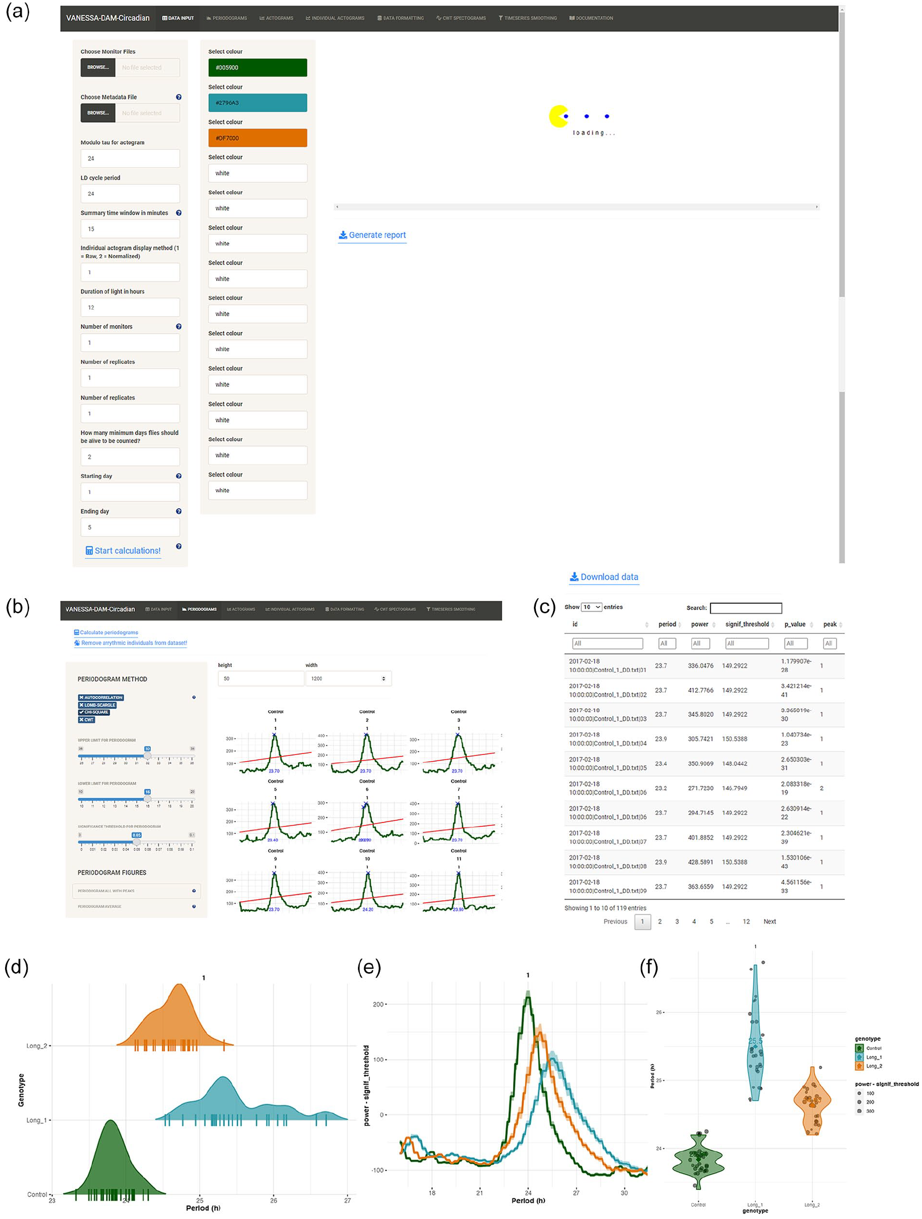
General description and period-power calculation in VANESSA-DAM. (a) The home tab of VANESSA-DAM—the Data Input tab. This tab has different parameters that can be changed according to the user’s analysis needs—modulo-Tao, the LD cycle period in the experiment, summary time window, light duration, total number of monitors being analyzed, replicate declaration, subset data to specific days and indicate for how many days flies must be alive to be included in calculations and plots. This tab can also be used to customize colors for different identifiers. (b) Examples of periodogram calculations using chi-square method from the “Periodogram” tab. Users can easily define upper and lower limits of periods to be scanned and also define significance threshold for the periodogram method. (c) Example of a preview of the tabulated data file that can be downloaded with all period and power values for all individuals for all significant peaks in periodogram. (d) Example of a density plot of period values of individuals from different identifiers. All individual period values are plotted as short horizontal lines-“|” on the x-axis. (e) Average periodogram of all individuals from different identifiers. (f) Violin plot of period values of all individuals from different identifiers are plotted along with the mean period value of that identifier embedded in the plot.

Vanessa-Dam-Cra–Specific Features

Periodograms

Four popular periodogram methods have been incorporated in the app-(a) autocorrelation, (b) chi-square (greedy chi-square method, improved method over the classical chi-square method), (c) Lomb–Scargle, and (d) continuous wavelet transformation (CWT) (Figure 1c and 1d). Users can choose upper limit, lower limit, and significance threshold for the periodogram analysis for all methods (Figure 1c). Arrhythmic individuals can be removed from the data set after determining periodicity so that they do not affect further analysis and visualization of average profiles, average periodograms, and batch actograms. All period and power values of each individual can be downloaded as csv files where different peaks of periodograms for all individuals will be saved (Figure 1d). Four useful visualizations are provided for period data-(a) all individual periodograms can be plotted captioned with monitor and channel number, identifier, and replicate number with user specified colors of the particular identifiers; the highest peak of the periodograms will be identified and printed in these plots, (b) periodograms can be averaged over individuals of an identifier and plotted, (c) violin plots of all identifiers can be plotted along with individual data points and the mean of each identifier will be calculated and printed on the plots, (d) a density plot of periods of identifiers can be plotted along with individual period values on the x-axis (Figure 1e-1g).

Actograms and Average Profiles

Activity counts can be visualized as heatmap “ethograms” for raw data and curated data (Figure 2a). All double-plotted actograms for all individuals can be visualized either together enabling quick and clear visualization of individuals that exhibit abnormal/unique and thus interesting patterns of activity, or separately, one-by-one along with their periodograms displayed below them enabling ease of picking representative actograms (Figure 2b and 2c). Double-plotted batch actograms are also available for each identifier separately (Figure 2g). Average profiles for individuals and all individuals of an identifier can be visualized either as a time series of consecutive days or averaging across days (Figure 2e). Average profiles of activity can also be visualized via a circular plot for each identifier (Figure 2d). All these plots can be plotted either with raw activity counts or with normalized activity (Figure 2f and 2h).

Figure 2.

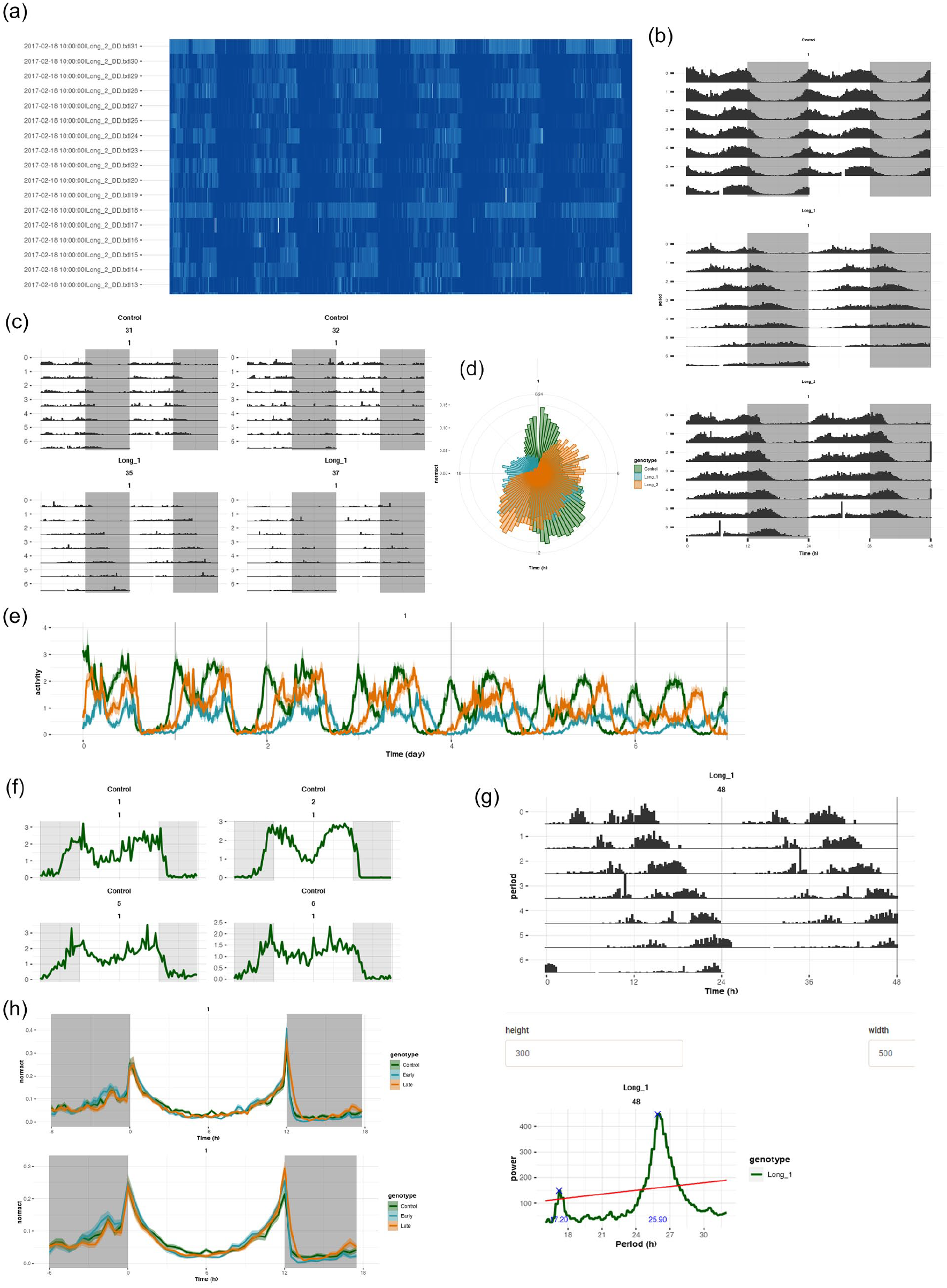
Actograms and activity profile visualization in VANESSA-DAM-CRA. (a) Activity profiles plotted as an ethogram where darkest blue color depicts highest activity and complete white indicates zero activity. Ethograms are an easy way to look at data from all individuals at a glance and notice any abnormal or unexpected patterns. (b) Batch actograms of different identifiers. The light–dark shading can be quickly altered by changing the “Duration of light in hours” parameters in the “Data input” tab. (c) Actograms of all individuals of one identifier can be visualized together. (d) Average activity profiles can also be visualized in a polar scale. (e) Day-wise activity profiles for all identifiers can be plotted averaged across individuals. (f) Activity profiles of each individual averaged across days can also be visualized separately. (g) A separate tab, “Individual actograms,” can help visualize and inspect each actogram individually for the purpose of choosing representative actograms along with their periodograms. (h) Average activity profile of different identifiers can be plotted first averaged across days for each individual, then averaged across individuals. The top panel is plotted in 15 min bin and the bottom panel is plotted in 30 min bin. This binning can be changed quickly by changing the values of the “Summary time window in minutes” parameter in the “Data input” tab.

CWT Spectrogram and Time-series Smoothing

CWT spectrograms can be visualized for individuals over several days (Supplementary Methods 2-Step 18). This function does not require the metadata file; instead, the input is the monitor file itself. Wavelet powers for different periods scanned can also be visualized. The time-series smoothing function operates as a separate module and takes one single monitor file as input (Supplementary Methods 2-Step 19). Users can upload a monitor file, change the binning of the data, use 2 popular methods of time-series smoothening (lowpass Butterworth filter and kernel smoothing). For Butterworth filter, users can change “filter order or generic filter model” and “critical frequencies of the filter” and immediately check the effect of the binning and filtering on average profile of individuals of the monitor and on the individual profiles and download the smoothened data with applied parameters. Similarly, for kernel smoothing, users can specify the “kernel smoothing bandwidth.”

Vanessa-Dam-Sa–Specific Features

Sleep Profiles

Sleep bouts of each individual can be visualized as heatmaps across days. The other methods of sleep bout visualization are (a) plots of sleep bouts across days for each individual, (b) sleep bouts can be averaged across chosen days for each individual and plotted, (c) sleep bouts of individuals of an identifier can be averaged over chosen days and plotted, (d) sleep bouts can be first averaged across days for each individual and then averaged across individuals of an identifier and plotted in a linear manner or in a circular scale (Figure 3a-3g).

Figure 3.

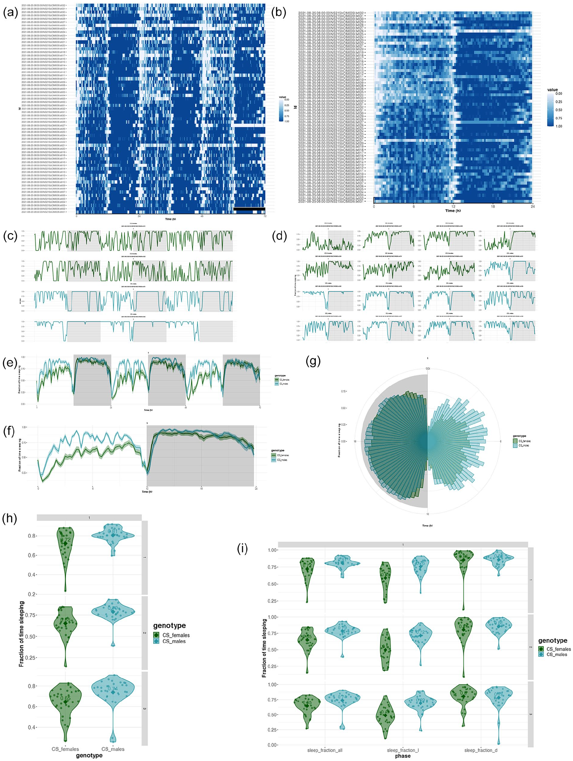
Somnograms and sleep fraction analyses in VANESSA-DAM-SA. (a) Somnogram of all individuals across different days selected can be visualized where clearest white color depicts zero sleep and darkest blue denotes maximum sleep. (b) Somnogram of all individuals averaged across selected days can be visualized where clearest white color depicts zero sleep and darkest blue denotes maximum sleep. (c) Day-wise sleep profiles of each individual from different identifiers can be plotted separately. (d) Sleep profiles of each individual averaged across selected days can be plotted. (e) Day-wise sleep profiles of each identifier averaged across all individuals. (f) Sleep profiles of each identifier first averaged across individuals then averaged across selected days. (g) Sleep profiles of each identifier first averaged across individuals then averaged across selected days in polar scale. (h) Fraction of time sleeping for each individual during the entire day for different identifiers as a violin plot for each day separately. (i) Fraction of time sleeping for the whole day (sleep_fraction_all), only in the light part of the day (sleep_fraction_l), and only in the dark part of the day (sleep_fraction_d) of each individual of different identifiers as a violin plot for each day separately.

Sleep Fractions, Bout, and Latency Analysis

Sleep analysis results such as sleep levels, bout details, latency data can be downloaded as csv files for all individuals separately for light and dark phases. Total sleep fractions and total sleep times of different identifiers for chosen days can be plotted as violin plots. Sleep fractions and total times in the light and dark part of the day can also be plotted for different identifiers as violin plots. Bout analysis can be visualized in different ways-(a) sleep and awake bouts can be plotted for individuals of an identifier, (b) violin plot of number of sleep and awake bouts for an identifier, (c) violin plot of mean sleep and awake bout lengths for an identifier, (d) violin plot of sleep latency for an identifier, (e) for all measurements, light and dark phase values can be plotted as separate violin plots (Figures 3h and 3i, 4a-4k).

Figure 4.

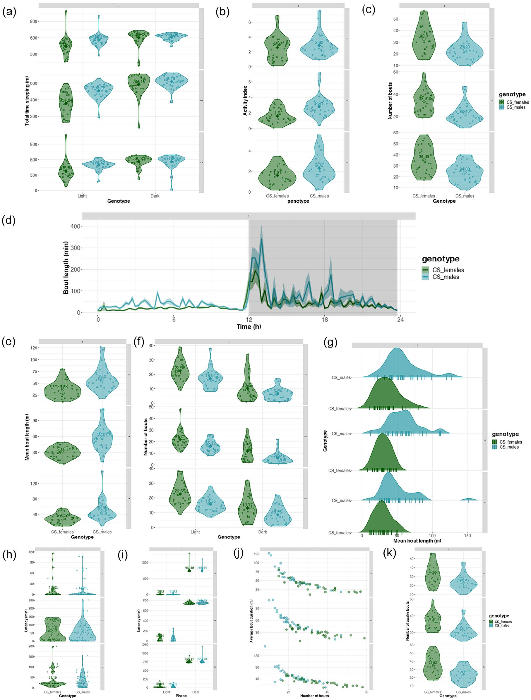
Sleep time, bout, and latency analyses in VANESSA-DAM-SA. (a) Total time sleeping in the light part of the day (light) and in the dark part of the day (dark) of each individual of different identifiers as a violin plot for each day separately. (b) Activity index (activity count per waking minute) of each individual of different identifiers as a violin plot for each day separately. (c) Violin plot of total number of bouts of all individuals of each identifier for each day separately. (d) Starting time of bout and bout lengths in minutes are plotted averaged across all individuals of each identifier. (e) Violin plot of mean bout length in minutes of all individuals of each identifier for each day separately. (f) Violin plot of number of bouts in dark (D) and light (L) parts of the day of all individuals of each identifier for each day separately. (g) Density plot of mean bout lengths in minutes for each identifier and mean bout lengths for each individual plotted along the x-axis for each day separately. (h) Violin plot of latency to first bout in minutes of all individuals of each identifier for each day separately. (i) Violin plot of latency to first bout in minutes in dark (D) and light (L) parts of the day of all individuals of each identifier for each day separately. (j) Plot of average bout duration in minutes versus number of bouts for all individuals colored by identifiers. (k) Violin plot of total number of awake bouts of all individuals of each identifier for each day separately. Note. Latency calculated as the time taken to the first sleep bout from ZT00.

Reproducible Codes

Both apps have capability of generating HTML files with all parameters used by the user for analysis in the session and codes to reproduce the same exact analyses to generate the tables and plots (Figure 5a-5c). Advanced users can tweak different codes for analyses to suit their needs and generate custom plots. For time-series smoothing, a HTML report file is generated with all parameters used for reproducing similar smoothing and binning of data.

Figure 5.

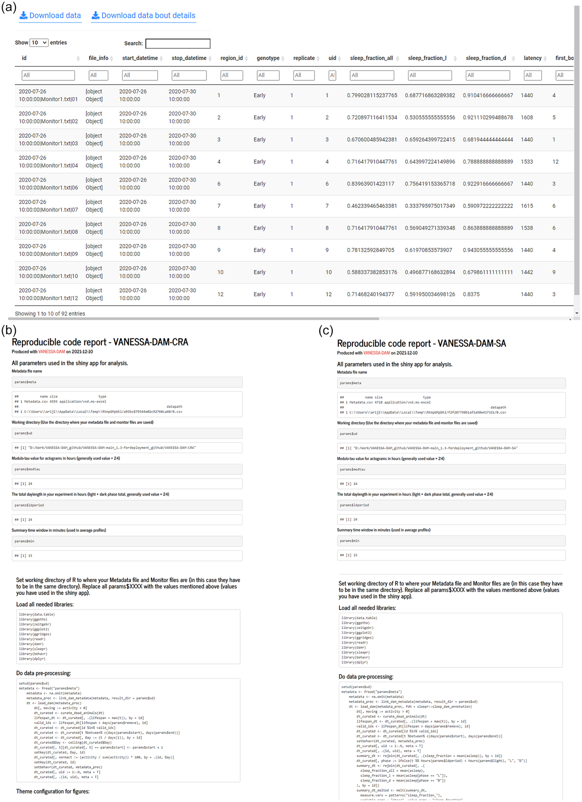
Examples of downloadable sleep analysis data and reproducible code reports from VANESSA-DAM. (a) Example of the tabulated sleep analysis data that can be downloaded from VANESSA-DAM-SA. (b) Snippets of reproducible code report with all used parameters for analysis to reproduce exact same analysis and plots from VANESSA-DAM-CRA. (c) Snippets of reproducible code report with all used parameters for analysis to reproduce exact same analysis and plots from VANESSA-DAM-SA.

The codes for these apps are hosted on GitHub (https://github.com/orijitghosh/VANESSA-DAM) and freely available under an MIT license along with toy/demo data. The apps are also hosted on a server and can directly be used from a browser with Internet connection (https://cryptodice.shinyapps.io/vanessa-dam-cra/ and https://cryptodice.shinyapps.io/vanessa-dam-sa/). In addition, VANESSA is available from GitHub as R packages and the instructions and usage are on the VANESSA-DAM GitHub page. VANESSA is also easily extendable to analyze locomotor activity data or any other numerical rhythmic behavioral data from other organisms recorded with systems other than DAM, and we will try our best to provide support for converting user data to DAM compatible files. Such an example is available in the Supplementary Materials (Suppl. Fig. 1) where mouse locomotor activity data recorded with Trikinetics software was easily converted to VANESSA compatible files easily with a few lines of code. We plan to host an online webserver for converting other format data to VANESSA compatible files, as and when we get requests from users. For now, only mouse data conversion is in place as a function from the vanessadamcra package. VANESSA is easily extendable to analysis of ultradian or infradian rhythms and, with a few modifications, can be used for analyzing rhythms other than locomotor activity. We welcome feature requests, suggestions, bug reports, and collaborations via GitHub or email. We have provided tips regarding interpretation of different plotting options, proper usage of different periodogram methods with appropriate parameters in the VANESSA-DAM wiki (https://github.com/orijitghosh/VANESSA-DAM/wiki/Good-practices/). We believe VANESSA apps will be extremely useful to fly circadian rhythm and sleep researchers, especially those working with high-throughput behavioral screenings where analyses need to be automated, and reproducibility of analysis methods is critical. Future updates will include but not be limited to calculation of the angle-doubled center of mass for bimodal actograms, support of generating metadata file for more than 12 monitor files, in-built statistical tests, subjective and objective phase marking, support for more data acquisition systems for more organisms, sleep analysis in specific time windows, and so on.

Supplemental Material

sj-pdf-1-jbr-10.1177_07487304221077662 – Supplemental material for VANESSA—Shiny Apps for Accelerated Time-series Analysis and Visualization of Drosophila Circadian Rhythm and Sleep Data

Supplemental material, sj-pdf-1-jbr-10.1177_07487304221077662 for VANESSA—Shiny Apps for Accelerated Time-series Analysis and Visualization of Drosophila Circadian Rhythm and Sleep Data by Arijit Ghosh and Vasu Sheeba in Journal of Biological Rhythms