Sage Journals: Discover world-class research

Abstract

Circadian rhythms are daily oscillations in physiology and behavior that can be assessed by recording body temperature, locomotor activity, or bioluminescent reporters, among other measures. These different types of data can vary greatly in waveform, noise characteristics, typical sampling rate, and length of recording. We developed 2 Shiny apps for exploration of these data, enabling visualization and analysis of circadian parameters such as period and phase. Methods include the discrete wavelet transform, sine fitting, the Lomb-Scargle periodogram, autocorrelation, and maximum entropy spectral analysis, giving a sense of how well each method works on each type of data. The apps also provide educational overviews and guidance for these methods, supporting the training of those new to this type of analysis. CIRCADA-E (Circadian App for Data Analysis–Experimental Time Series) allows users to explore a large curated experimental data set with mouse body temperature, locomotor activity, and PER2::LUC rhythms recorded from multiple tissues. CIRCADA-S (Circadian App for Data Analysis–Synthetic Time Series) generates and analyzes time series with user-specified parameters, thereby demonstrating how the accuracy of period and phase estimation depends on the type and level of noise, sampling rate, length of recording, and method. We demonstrate the potential uses of the apps through 2 in silico case studies.

Keywords

circadian rhythms biological oscillations data analysis discrete wavelet transform periodogram mathematical analyses Shiny app

Circadian rhythms are daily oscillations in physiology and behavior that continue in the absence of time cues and that have been widely observed in bacteria, archaea, fungi, plants, and animals (Hurley et al., 2016). In mice, for example, these rhythms can be observed in body temperature, locomotor activity, bioluminescent reporters of gene expression, and other measures (Leise et al., 2018). These different types of data vary greatly in waveform, noise characteristics, sampling rate, and length of recording. For instance, activity recordings often have high sampling rates, long durations, and square-like waveforms, while bioluminescence recordings tend to be sinusoid-like and only a few days in length. We developed 2 Shiny apps for exploration of these circadian data, enabling visualization and analysis of circadian parameters such as period and phase. Shiny is an R package supporting the creation of open-source interactive web apps (https://shiny.rstudio.com/). The motivation behind our apps is 2-fold: first, to create accessible tools for exploration and analysis of multiple forms of circadian data, and second, to develop an education resource for circadian data analysis. The original apps were developed by the 3 undergraduate authors L.C., L.K., and C.L. at Amherst College with extensive feedback and testing provided by undergraduates at Smith College, with the app development itself providing multiple valuable educational opportunities, including learning how to code in R and Shiny, how to communicate across the quantitative and life sciences, and how to create effective visualizations of data.

Five widely used estimation methods are included in the apps as a representative set of distinct analysis tools: the discrete wavelet transform (DWT), sine fitting, the Lomb-Scargle periodogram, autocorrelation, and maximum entropy spectral analysis (see Table 1 and the Methods section). The focus is on methods applicable to recordings of body temperature, locomotor activity, and bioluminescent reporters, such as PER2::LUC, with at least 3 days of data sampled at least once per hour. The analyses considered here are not aimed at, for instance, detection of circadian rhythms in transcriptome or proteome data, which tend to have short duration and sparse sampling and for which appropriate tools are freely available, including JTK_Cycle (Hughes et al., 2010), RAIN (Thaben and Westermark, 2014), MetaCycle (Wu et al., 2016), and LimoRhyde (Singer and Hughey, 2019), among others. Our educational apps complement existing circadian data analysis apps, such as Biodare (Zielinski et al., 2014), CATkit (Gierke and Cornelissen, 2016), Rethomics (Geissmann et al., 2019), and RhythmicAlly (Abhilash and Sheeba, 2019), by training users to be more knowledgeable in how best to use and interpret different types of analyses for a variety of data types.

Table 1.

Summary of methods available in CIRCADA apps.

Method	Purpose	References	Notes
Discrete wavelet transform (DWT)	Removal of noise and/or trend; estimates of peak times and heights	Leise and Harrington, 2011; Leise, 2015; Samar et al., 1999; Torrence and Compo, 1998	May need to discard first and last day due to edge effects; sampling rate determines period bands; best if time series has at least 5 cycles
Autocorrelation	Evidence of rhythmicity via rhythmicity index; period estimate	Chatfield, 2004, p22-28; Dowse, 2009; Levine et al., 2002	Works well for any waveform; should detrend first; good initial test to apply in examining a possibly rhythmic time series; best if time series has at least 4 cycles
Sine fitting	Estimates of period, phase, and amplitude	Cornelissen, 2014; Cohen et al., 2012; Refinetti et al., 2007; Halberg et al., 1967	Can be used on nonuniformly sampled data; works best for sinusoidal waveforms; typically good to detrend before applying
Lomb-Scargle periodogram	Estimate of period; statistical test for significance	Glynn et al., 2005; Ruf, 1999; VanderPlas, 2018; Lomb, 1976	Can be used on nonuniformly sampled data; can use randomization to generate p values if assumptions are not met for theoretical formula
Maximum entropy spectral analysis	Estimate of period	Dowse, 2009; Dowse, 2013; Ulrych and Bishop, 1975	No significance test; higher resolution estimates than Fourier periodogram

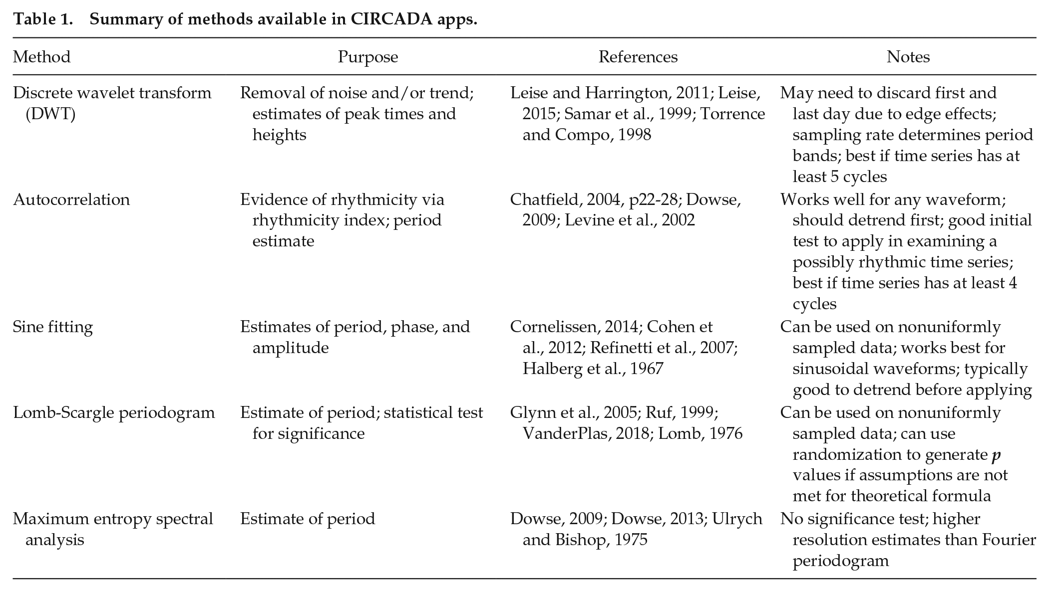
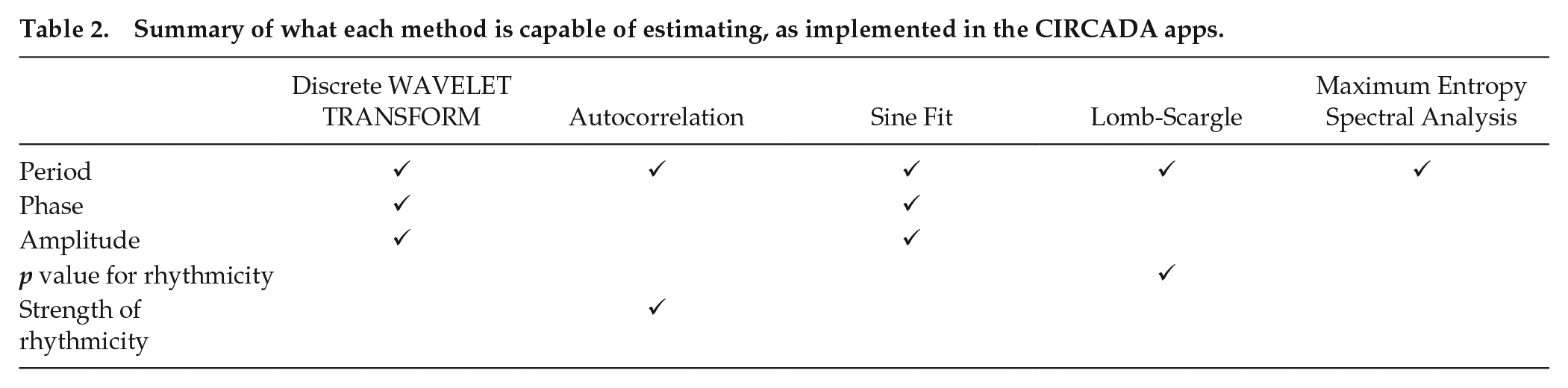
The 5 methods use quite different approaches to estimating rhythmic characteristics of time series and produce different subsets of the desired information about the time series, as shown in Table 2. All 5 methods generate estimates of the period (cycle length), but not all estimate the phase (reported as the peak time) and the amplitude (defined as half the peak-to-trough distance). The Lomb-Scargle method provides a p value for the significance of the dominant periodicity, and autocorrelation provides a measure of the strength of rhythmicity (rhythmicity index). Some methods may have biases, depending on the waveform, trend, and type of noise, and the methods exhibit differences in accuracy of the estimates that depend on these time series characteristics. For example, sine fitting assumes a symmetric waveform and so may produce a peak time estimate that is too late for a waveform that rises sharply then gradually decreases. These differences can sometimes be hard to predict, as the underlying theory generally assumes no trend and simple Gaussian noise. By providing results and visualizations of the application of these 5 methods to a variety of data types, the CIRCADA apps allow their effectiveness to be assessed for each case.

Table 2.

Summary of what each method is capable of estimating, as implemented in the CIRCADA apps.

	Discrete WAVELET TRANSFORM	Autocorrelation	Sine Fit	Lomb-Scargle	Maximum Entropy Spectral Analysis
Period	✓	✓	✓	✓	✓
Phase	✓		✓
Amplitude	✓		✓
p value for rhythmicity				✓
Strength of rhythmicity		✓

The first app, CIRCADA-E (Circadian App for Data Analysis–Experimental Time Series; see Supplemental Fig. 1), allows users to explore a large set of data from Leise et al. (2018) with mouse body temperature, locomotor activity, and PER2::LUC recordings from multiple tissues (publicly accessible at https://osf.io/seyhp/). Samples from old and young mice under 24-h and 20-h T-cycles on normal and high-fat diets are available in these data. In our experience, finding large, interesting, public data sets in a usable form for undergraduate courses can be challenging. By directly interfacing a rich data set with multiple methods of analysis and visualization in a user-friendly app, CIRCADA-E supports a variety of training and educational activities. For instance, students learning to work in a circadian lab can practice generating and testing hypotheses about circadian rhythm measures using this curated set of data with built-in analysis. Possible student projects include comparing distributions of body temperature periods for animals under the 24-h versus 20-h T-cycles, comparing period and peak time estimates for body temperature versus locomotor activity rhythms, or practicing analysis of results from 2 × 2 or 2 × 2 × 2 factorial design experiments by testing for differences in the rhythmicity index of the SCN in vitro rhythms or in the amplitude of the body temperature rhythms. The app also facilitates direct comparison of the results of different methods to assess which might work best for a particular type of data and how accurate and reliable those results may be. Visualization is a major feature of the apps, with graphs of raw data, processed data, and outputs of each method, encouraging regular visual checking of whether results appear consistent with the data.

The second app, CIRCADA-S (Circadian App for Data Analysis–Synthetic Time Series; see Supplemental Fig. 2), generates and analyzes time series with user-specified parameters, listed in Table 3. CIRCADA-S can be used to explore how accuracy of period and phase estimation depends on sampling rate, length of recording, type and level of noise, and method used. This app also offers educational overviews and guidance for each method to provide further training support. As an example, Supplemental Figure 2 displays the CIRCADA-S Lomb-Scargle tab, which demonstrates how increasing the oversampling factor increases resolution of the period estimate and provides a link to a popup window with explanatory details about the method. Results from the 5 methods for a set of generated time series samples are summarized in the CIRCADA-S Summary tab, shown in Figure 1, including histograms of the period errors to facilitate comparison. For example, the DWT, autocorrelation, and Lomb-Scargle methods produce highly discretized period estimates, with the discrete values depending on the sampling interval length for DWT and autocorrelation and more heavily on the number of cycles for the Lomb-Scargle. In contrast, sine fitting and maximum entropy spectral analysis (MESA) generate more fine-grained estimates with resolution independent of sampling interval and number of cycles, with sine-fitting estimates more tightly clustered compared with MESA. Note that higher resolution does not necessarily correlate with higher accuracy of period estimation. As another example, Supplemental Figure 3 shows part of the CIRCADA-S DWT tab with an interactive demonstration of the DWT time series decomposition (which is also available in CIRCADA-E). There is also an Advice tab with suggested guidelines for using each method and brief glossary of the user-set parameter options.

Table 3.

User choices for generating synthetic data in CIRCADA-S.

Parameter	Range of Values
Sampling interval	0.125, 0.25, 0.5, 1, or 2 h
Mean period	20-28 h
Standard deviation (SD) of periods	0-2 h
Peak location	0-1 (any proportion of a cycle)
Amplitude	0-3 (arbitrary units)
Waveform	Sinusoid, square wave, or asymmetric triangular wave
Noise standard deviation	0-3 (arbitrary units)
Noise type	Gaussian, pink, brown, or scaled by the signal
Trend	None, linear, or quadratic
No. of samples	1-1000

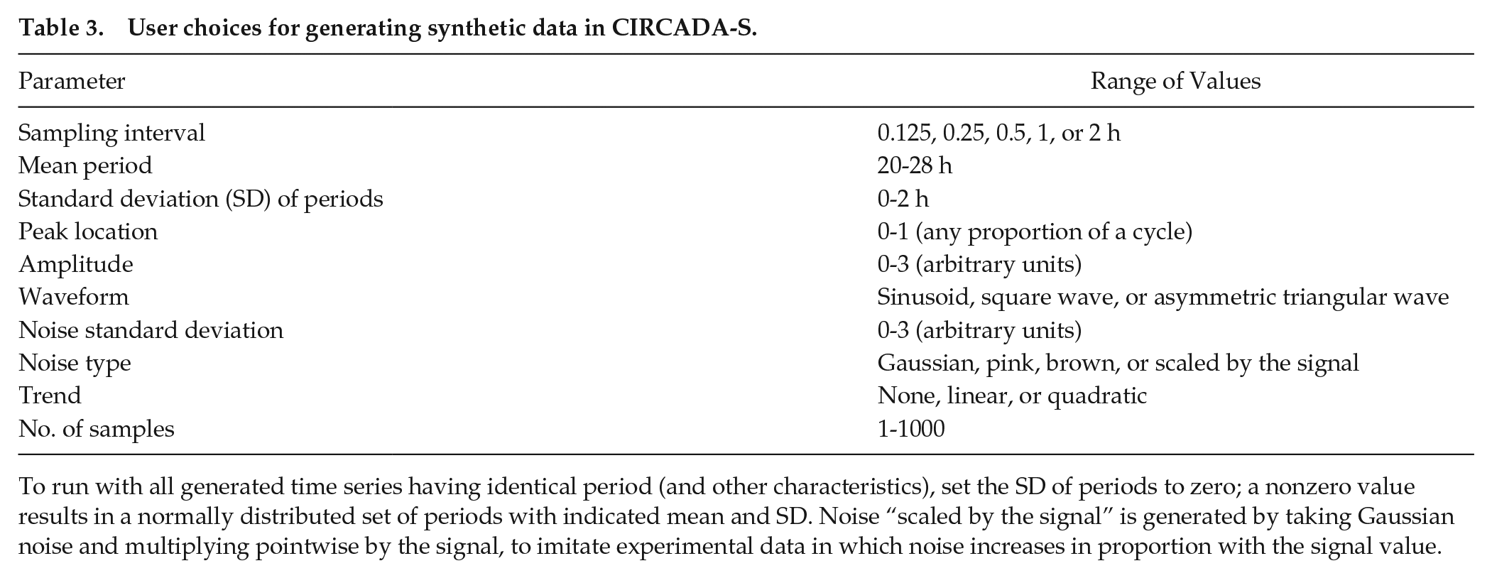
To run with all generated time series having identical period (and other characteristics), set the SD of periods to zero; a nonzero value results in a normally distributed set of periods with indicated mean and SD. Noise “scaled by the signal” is generated by taking Gaussian noise and multiplying pointwise by the signal, to imitate experimental data in which noise increases in proportion with the signal value.

Figure 1.

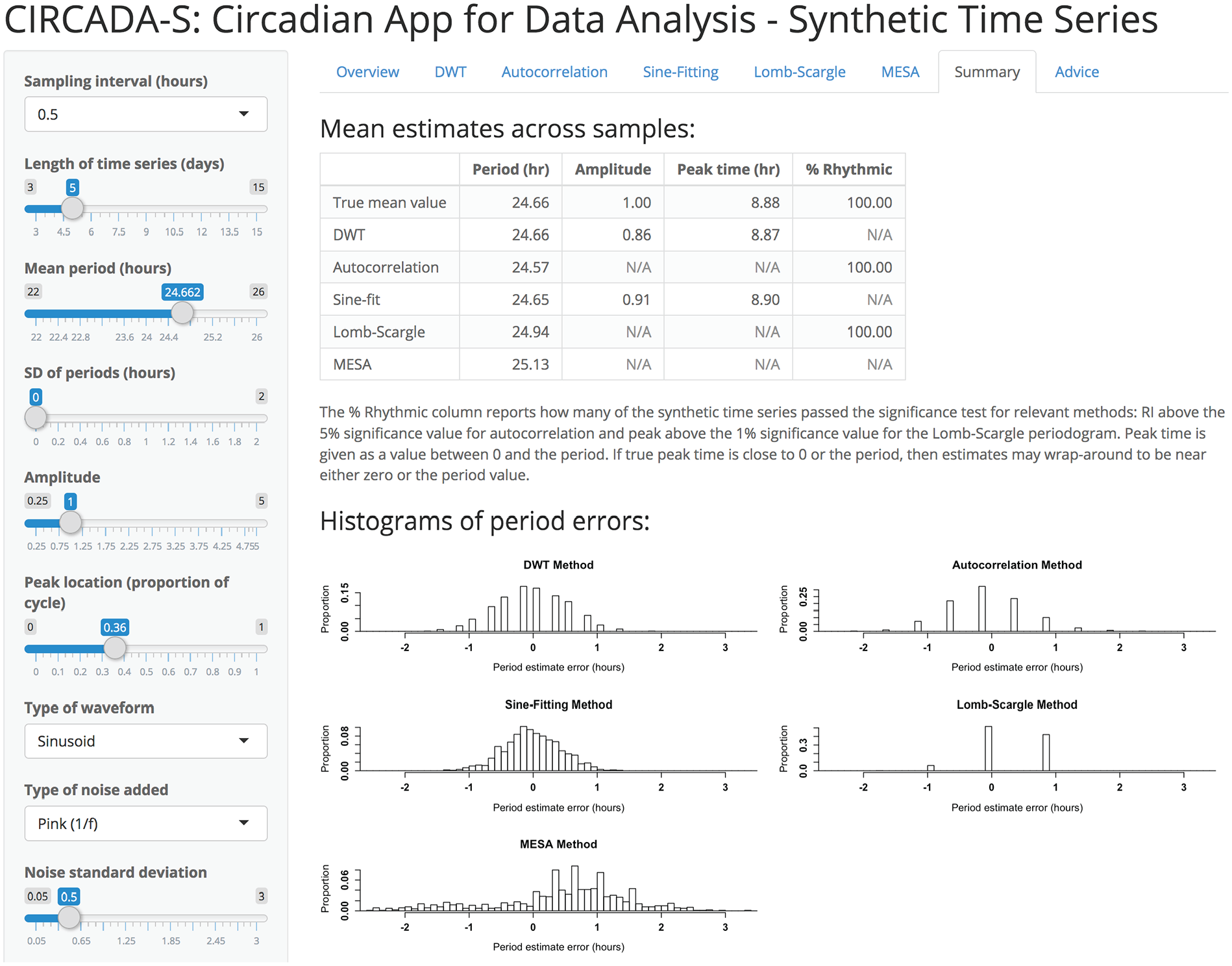
Partial screenshot of CIRCADA-S Summary tab, comparing results from the five methods for a set of 1,000 generated time series with the user-selected characteristics. The histograms of period errors demonstrate the differences between the methods. The DWT, autocorrelation, and Lomb-Scargle produce discrete estimates with possible values determined by the sampling interval and number of cycles, while sine-fitting and MESA produce finer-grained estimates.

Use in Varied Educational Settings

To better understand how these apps might be used, we applied them in a variety of educational settings. In a very introductory class, CIRCADA-S was used within a classroom demonstration to help students understand the Lomb-Scargle periodogram. In a more advanced course, CIRCADA-E was used by a student to address a research question about the interaction of light cycles on body temperature cycles. Within an undergraduate chronobiology research lab, all students completed an online exercise with brief quizzes to guide their exploration of CIRCADA-E. In a week-long chronobiology course for graduate students, CIRCADA-E was used to help students create simulated data with characteristics of their own data set, and results from the simulations were discussed in terms of how to select optimal data analysis tools. Students in all settings reported that this was a helpful tool and increased their understanding of methods to analyze rhythmic data. A sample online lesson, “Learning about the Analysis of Rhythmic Data,” which guides new users through the apps and methods, is posted on the Open Science Framework (OSF) site (https://osf.io/er6wj/), with checkpoint questions at regular intervals to support self-testing for comprehension.

In Silico Case Study: Sampling Rate Versus Duration

To demonstrate the effect of sampling rate versus duration of the time series on period estimate accuracy, we generated 1000 noisy sinusoids with a sampling interval of 0.125 h for 16 days. The time series were subsampled to generate larger sampling intervals, and days were dropped from the end to generate shorter durations. Results for the sine-fitting and Lomb-Scargle methods are shown in Figure 2 as examples. Each additional day in the time series tends to have a greater effect in increasing accuracy than does shortening the time step. For example, the period error in the sine-fit estimates is reduced by nearly 50% by going from 3 days to 5 days (requiring 36 versus 60 time points for 2-h sampling), while increasing the sampling from once every 2 h to 8 times an hour for 3 days (36 versus 576 time points) reduces the error by only about 16%.

Figure 2.

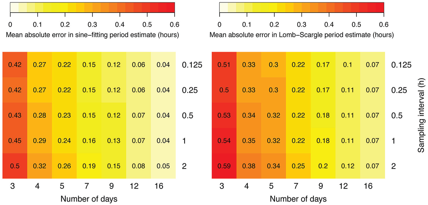
Errors in estimating period using sine-fitting (left) and Lomb-Scargle (right) methods for 1000 noisy sinusoids with normally distributed periods (mean 24 h, SD 0.5 h), amplitude 1, noise standard deviation 0.5 with pink noise, and quadratic trend, for indicated number of days and sampling interval.

In Silico Case Study: Statistical Power

CIRCADA-S can also be used to study how many samples might be necessary to achieve sufficient statistical power in an experiment, given a fixed duration and sampling interval. Sets of synthetic time series with characteristics selected to be similar to those of the experimental data can be generated to estimate the likely statistical power for different numbers of samples, for example, to detect a difference in period between 2 groups. See Figure 3 for an example showing that the addition of a cycle to the data can greatly strengthen the power and reduce the number of samples needed. Results of the app’s analysis are automatically downloaded to a file named CIRCADA-S-output.csv to facilitate this type of further exploration.

Figure 3.

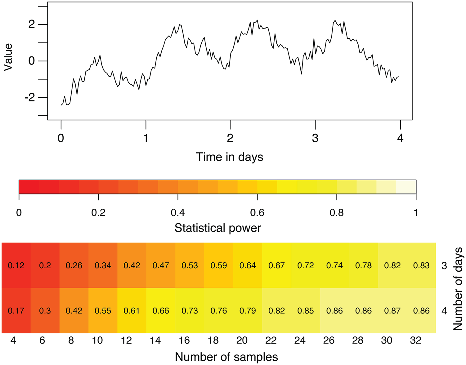
Power study using generated time series. Top: example of a 4-day noisy sinusoid. Bottom: Probability of detecting a significant different in sine-fit period between 2 groups for the indicated number of samples and length of time series (using t.test in R), where the true means are 23.35 and 23.85 h. Periods within each group are normally distributed, with a standard deviation of 0.25 h, amplitude of 1, noise is pink, with standard deviation is 0.5, trend is quadratic, and a sampling interval is 0.5 h. About 30 samples would be needed to obtain a statistical power of 0.80 using a 3-day duration, while increasing the duration to 4 days substantially decreases the required sample size to just greater than 20.

Running CIRCADA

To run the apps, download and save the compressed CIRCADA folder from https://osf.io/er6wj/ to your computer, then open CIRCADA-E.R or CIRCADA-S.R in RStudio and click “Run app.” All required packages will be installed as needed by running the app. A tutorial (GettingStarted.pdf) is available at https://osf.io/er6wj/ for learning the features of the apps and includes suggestions for training activities and projects. An online lesson is also provided on the OSF site.

Methods

The Shiny code for both apps is freely available at https://osf.io/er6wj/, with easily adaptable R code provided for each of the methods. Figures were generated using R 3.5.3 (https://www.r-project.org/) in RStudio 1.2.1335 (https://www.rstudio.com/). Experimental data used in CIRCADA-E are from Leise et al. (2018), using methods as described in that article where they overlap with those used in the app. The data are accessed from the OSF site https://osf.io/seyhp/ using the osfr R package (https://github.com/CenterForOpenScience/osfr). The R code used to analyze that data in batch form is also available in Rmarkdown format at https://osf.io/seyhp/.

Discrete Wavelet Transform

Time series are detrended using the DWT before applying other methods (with the exception that linear detrending is used if the time series covers 4 days or less). The apps use the function wavMRDSum from the wmtsa R package (https://cran.r-project.org/web/packages/wmtsa/) to calculate details, smooths, and their sums. The s12 filter is used for the DWT, with the exception that s8 is used if fewer than 120 time points are present. To avoid edge effects, portions are removed from each end after detrending, depending on the total length of the time series (8 h if only 3 days; 12 h if 4 days; 18 h if 5-6 days; 36 h if 7 or more days). Because some edge-effected intervals may still be present in the shorter time series, the DWT is more appropriate for time series with at least 5 cycles, preferably at least 7, so that edge effects can be fully removed while leaving multiple cycles for analysis. The DWT period estimate is the mean peak-to-peak time, and the peak time estimate is the circular mean of the peak times, converted to radians using the estimated period using the CircStats R package (https://cran.r-project.org/web/packages/CircStats/). The DWT amplitude estimate is the mean peak height.

Autocorrelation

The R command acf from the stats R package (https://stat.ethz.ch/R-manual/R-devel/library/stats/html/00Index.html) is used to calculate the autocorrelation of detrended time series. The maximum peak in the autocorrelation corresponding to a lag between 12 h and 40 h is used to estimate the period and rhythmicity index, after first convolving with (1/8, 1/4, 1/4, 1/4, 1/8) to smooth the correlogram.

Sine Fitting

The R command nls (nonlinear least squares) from the stats R package is used to fit the 3 parameters of the sinusoidal curve to each time series. These parameters are then converted to amplitude, period, and phase angle for use in reporting estimates. Each fit is run 8 times for different initial parameter values, and the best fit (smallest root mean square error) is chosen.

Lomb-Scargle Periodogram

The R command lsp is used to calculate the Lomb-Scargle periodogram, from the lomb R package (https://cran.r-project.org/web/packages/lomb). The highest peak corresponding in the period range of 16 to 34 h is chosen as the period estimate. Higher period resolution may be obtained by increasing the oversampling factor, as shown in the periodogram in Supplemental Figure 2; oversampling factor 8 is used for the period estimate. In the CIRCADA-E app, the significance of peaks is assessed using a randomization procedure via randlsp, which produces a more valid result when the theoretical assumptions may not hold, such as normally distributed uncorrelated noise. However, the randomization procedure is computationally intensive, so the CIRCADA-S app runs it for only a representative time series and uses the theoretical p value for the full set of samples (which is a quick calculation). The time series is shuffled into a random order, for which a Lomb-Scargle estimate is generated. This process is repeated many times to generate a peak power distribution for shuffled time series (as shown in the histogram at the bottom of Supplemental Fig. 2), which can be used to estimate a p value: the probability that the Lomb-Scargle estimate for the original time series occurred by chance. Using randomization to calculate the p value is computationally intensive because it requires many repetitions to generate a sufficient distribution; 1000 are used in the apps, the minimal number for reasonable estimates, which in practice tend to be similar to the theoretical values. For example, for the representative synthetic time series in Supplemental Figure 2, the theoretical threshold value of 6.31 for a significance level = 0.01 (reported in the app tables and shown as a horizontal orange line in the periodogram) is near the value generated by the randomization method, indicated by the vertical orange line in the lower histogram.

MESA

The R command spec.ar from the stats R package is used to compute the MESA periodogram, using the Yule-Walker method with order 48/TimeStep. The number of frequencies checked is 2^(5+ceiling(log2(N))), where N is the number of time points. The highest peak corresponding to the period between 16 h and 34 h is chosen as the period estimate.

Generation of Random Time Series

Each sample time series in CIRCADA-S is the sum of a periodic function plus random noise plus trend. The periodic function has period $τ$ equal to a normally distributed random number with the selected mean and standard deviation (all samples will have the same period if the standard deviation is set to zero), user-selected amplitude A, and 1 of 3 waveforms, where $t_{p e a k}$ is the time of the first peak. The sinusoidal waveform is defined as $A \cos (2 π (t - t_{p e a k}) / τ)$ ; the square waveform is defined to be the step function that equals $2 A$ when time $t$ is within $τ / 4$ of a multiple of $τ$ , and zero otherwise; and the asymmetric triangular wave is a piecewise linear function with peak value $2 A$ at time $t_{p e a k}$ , decreases linearly down to equal zero at time $t_{p e a k}$ + $τ / 2,$ remains at zero until time $t_{p e a k} + 5 τ / 6,$ at which point it increases linearly to equal $2 A$ at time $t_{p e a k} + τ$ , then repeats periodically every $τ$ hours. For Gaussian noise, a vector of normally distributed random numbers has a mean 0 and standard deviation as selected by the user; if noise scaled by the signal is selected, each value in this vector is multiplied by the corresponding value of the time series minus the overall minimum value, divided by the mean difference from the minimum to normalize. For pink and brown noise, the R command noise is used from the package tuner, setting kind = “pink” and kind = “power” with alpha = 2, respectively. A linear trend is defined as $m t$ with slope $m$ randomly chosen between ½ and 2 divided by the total number of hours in the time series, equally likely to be positive or negative. A quadratic trend is defined as $a {(t - t_{0})}^{2}$ with coefficient $a$ randomly chosen between ½ and 2 divided by the square of half the total number of hours in the time series, equally likely to be positive or negative, and with vertex at $t_{0}$ randomly chosen near the center of the time series (between 10 and 14 times the number of days, where 12 times the number of days gives the center of the time series).

Packages Used by the CIRCADA Apps

Packages used include pracma (https://cran.r-project.org/web/packages/pracma/), tidyr (https://cran.r-project.org/web/packages/tidyr/), dplyr (https://cran.r-project.org/web/packages/dplyr/), data.tree (https://cran.r-project.org/web/packages/data.tree/), DiagrammeR (https://rich-iannone.github.io/DiagrammeR/), shinyjs (https://deanattali.com/shinyjs/), shinythemes (https://cran.r-project.org/web/packages/shinythemes/), DT (https://rstudio.github.io/DT/), remotes (https://cran.r-project.org/web/packages/remotes/), tuneR (https://cran.r-project.org/web/packages/tuneR/), and shinysky (https://github.com/AnalytixWare/ShinySky/wiki).

Supplemental Material

SupplementalMaterial-JBR-19-0114.R1 – Supplemental material for CIRCADA: Shiny Apps for Exploration of Experimental and Synthetic Circadian Time Series with an Educational Emphasis

Supplemental material, SupplementalMaterial-JBR-19-0114.R1 for CIRCADA: Shiny Apps for Exploration of Experimental and Synthetic Circadian Time Series with an Educational Emphasis by Lisa Cenek, Liubou Klindziuk, Cindy Lopez, Eleanor McCartney, Blanca Martin Burgos, Selma Tir, Mary E. Harrington and Tanya L. Leise in Journal of Biological Rhythms

Footnotes

Acknowledgements

We thank Dominica Cao, Yilin Cui, Hanxiao Lu, and Hannah Wang, for feedback and beta testing of the apps. The undergraduate research of L.C., L.K., and C.L. was supported by the Clare Boothe Luce Foundation and the Amherst College Gregory S. Call Undergraduate Research Fund. This work was supported by National Institutes of Health grants GM126545 and P01AG009975.

Conflict of Interest Statement

The authors have no potential conflicts of interest with respect to the research, authorship, and/or publication of this article.

ORCID iD

Tanya L. Leise

Notes

References

Abhilash

Sheeba

(2019) RhythmicAlly: Your R and Shiny-based open-source ally for the analysis of biological rhythms. J Biol Rhythms 34(5):551-561.

Chatfield

(2004) The analysis of time series. 6th ed. Boca Raton (FL): CRC Press.

Cohen

Leise

Welsh

(2012) Bayesian statistical analysis of circadian oscillations in fibroblasts. J Theor Biol 314:182-191.

Cornelissen

(2014) Cosinor-based rhythmometry. Theor Biol Med Model 11:16.

Dowse

(2009) Analyses for physiological and behavioral rhythmicity. Methods Enzymol 454:141-174.

Dowse

(2013) Maximum entropy spectral analysis for circadian rhythms: theory, history and practice. J Circad Rhythms 11:6.

Gierke

Cornelissen

(2016) Chronomics analysis toolkit (CATkit). Biol Rhythm Res 47:163-181.

Geissmann

Garcia Rodriguez

Beckwith

Gilestro

(2019) Rethomics: an R framework to analyse high-throughput behavioural data. PLoS One 14(1):e0209331. https://doi.org/10.1371/journal.pone.0209331

Glynn

Chen

Mushegian

(2005) Detecting periodic patterns in unevenly spaced gene expression time series using Lomb–Scargle periodograms. Bioinformatics 22:310-316.

10.

Halberg

Tong

Johnson

(1967) Circadian system phase, an aspect of temporal morphology: procedures and illustrative examples. In: von Mayersbach

, editor. The cellular aspects of biorhythms. Berlin: Springer. p. 20-48.

11.

Hughes

Hogenesch

Kornacker

(2010) JTK_CYCLE: an efficient nonparametric algorithm for detecting rhythmic components in genome-scale data sets. J Biol Rhythms 25(5):372-380.

12.

Hurley

Loros

Dunlap

(2016) Circadian oscillators: around the transcription–translation feedback loop and on to output. Trends Biochem Sci 41(10):834-846.

13.

Leise

(2015) Wavelet-based analysis of circadian behavioral rhythms. In: Sehgal

, editor. Methods in enzymology. San Diego (CA): Academic Press. p. 95-119.

14.

Leise

Goldberg

Michael

Montoya

Solow

Molyneux

Vetrivelan

Harrington

(2018) Recurring circadian disruption alters circadian clock sensitivity to resetting. Eur J Neurosci. In press.

15.

Leise

Harrington

(2011) Wavelet-based time series analysis of circadian rhythms. J Biol Rhythms 26:454-463.

16.

Levine

Funes

Dowse

Hall

(2002) Signal analysis of behavioral and molecular cycles. BMC Neurosci 3:1.

17.

Lomb

(1976) Least-squares frequency analysis of unequally spaced data. Astrophys Space Sci 39:447-462.

18.

Refinetti

Cornelissen

Halberg

(2007) Procedures for numerical analysis of circadian rhythms. Biol Rhythm Res 38:275-325.

19.

Ruf

(1999) The Lomb-Scargle periodogram in biological rhythm research: analysis of incomplete and unequally spaced time-series. Biol Rhythm Res 30(2):178-201.

20.

Samar

Bopardikar

Rao

Swartz

(1999) Wavelet analysis of neuroelectric waveforms: a conceptual tutorial. Brain Lang 66:7-60.

21.

Singer

Hughey

(2019) LimoRhyde: a flexible approach for differential analysis of rhythmic transcriptome data. J Biol Rhythms 34:5-18.

22.

Thaben

Westermark

(2014) Detecting rhythms in time series with RAIN. J Biol Rhythms 29:391-400.

23.

Torrence

Compo

(1998) A practical guide to wavelet analysis. Bull Am Meteorol Soc 79(1):61-78.

24.

Ulrych

Bishop

(1975) Maximum entropy spectral analysis and autoregressive decomposition. Rev Geophys Space Phys 13:183-300.

25.

VanderPlas

(2018) Understanding the Lomb–Scargle periodogram. The Astrophysical Journal Supplement Series 236:16.

26.

Anafi

Hughes

Kornacker

Hogenesch

(2016) MetaCycle: an integrated R package to evaluate periodicity in large scale data. Bioinformatics 32(21):3351-3353.

27.

Zielinski

Moore

Troup

Halliday

Millar

(2014) Strengths and limitations of period estimation methods for circadian data. PloS One 9(5):e96462.

Supplementary Material

Please find the following supplemental material available below.

For Open Access articles published under a Creative Commons License, all supplemental material carries the same license as the article it is associated with.

For non-Open Access articles published, all supplemental material carries a non-exclusive license, and permission requests for re-use of supplemental material or any part of supplemental material shall be sent directly to the copyright owner as specified in the copyright notice associated with the article.

0.00 MB

1.54 MB