Sage Journals: Discover world-class research

Abstract

The human circadian pacemaker entrains to the 24-h day, but interindividual differences in properties of the pacemaker, such as intrinsic period, affect chronotype and mediate responses to challenges to the circadian system, such as shift work and jet lag, and the efficacy of therapeutic interventions such as light therapy. Robust characterization of circadian properties requires desynchronization of the circadian system from the rest-activity cycle, and these forced desynchrony protocols are very time and resource intensive. However, circadian protocols designed to derive the relationship between light intensity and phase shift, which is inherently affected by intrinsic period, may be applied more broadly. To exploit this relationship, we applied a mathematical model of the human circadian pacemaker with a Markov-Chain Monte Carlo parameter estimation algorithm to estimate the representative group intrinsic period for a group of participants using their collective illuminance-response curve data. We first validated this methodology using simulated illuminance-response curve data in which the intrinsic period was known. Over a physiological range of intrinsic periods, this method accurately estimated the representative intrinsic period of the group. We also applied the method to previously published experimental data describing the illuminance-response curve for a group of healthy adult participants. We estimated the study participants’ representative group intrinsic period to be 24.26 and 24.27 h using uniform and normal priors, respectively, consistent with estimates of the average intrinsic period of healthy adults determined using forced desynchrony protocols. Our results establish an approach to estimate a population’s representative intrinsic period from illuminance-response curve data, thereby facilitating the characterization of intrinsic period across a broader range of participant populations than could be studied using forced desynchrony protocols. Future applications of this approach may improve the understanding of demographic differences in the intrinsic circadian period.

Keywords

mathematical model circadian intrinsic period human oscillator MCMC parameter estimation

Molecular clocks maintain an ~24-h rhythm in the firing rate of neurons in the suprachiasmatic nucleus (Belle et al., 2009; Welsh et al., 2010). The collective activity of these neurons gives rise to a circadian rhythm that acts as a pacemaker to coordinate biological rhythms throughout the body (Saper et al., 2005). The properties of this pacemaker, including its intrinsic period and amplitude, affect an individual’s phase of entrainment (Aschoff and Pohl, 1978; Wright et al., 2005; Granada et al., 2013; Bordyugov et al., 2015) and are thought to determine chronotype, a measure of an individual’s morningness/eveningness (Roenneberg et al., 2003). In addition, these properties affect an individual’s susceptibility to jet lag (Eastman et al., 2016), ability to tolerate shift work (Eastman et al., 2016), and response to circadian-based therapeutic interventions such as light therapy (Gooley, 2008). Furthermore, circadian properties may have implications for societal constructs such as appropriate work hours (Landrigan et al., 2007) and school start times (Carskadon et al., 2004; Danner and Phillips, 2008; Dunster et al., 2018).

Forced desynchrony (FD) protocols represent the gold standard methodology for assessing an individual’s intrinsic circadian period. In these protocols, circadian rhythmicity is desynchronized from sleep/wake behavior by imposing a regular light:dark (LD) cycle that is outside the range of entrainment of the circadian pacemaker. A marker of free-running circadian period, usually salivary or plasma melatonin or core body temperature, is used to estimate the pacemaker’s intrinsic period, τ (Carskadon et al., 1999; Czeisler et al., 1999). Using FD protocols, τ has been estimated to be 24.18 ± 0.04 h (mean ± SEM) in healthy young men (Czeisler et al., 1999), but the intrinsic period can vary based on many different factors including age, sex, and race/ethnicity (Carskadon et al., 1999; Smith et al., 2009; Duffy et al., 2011; Eastman et al., 2012; Eastman et al., 2015). In healthy adults, the intrinsic circadian period has been estimated to range from 23.5 h to 24.9 h (Smith et al., 2009; Duffy et al., 2011).

FD protocols are highly time and resource intensive with accurate assessments requiring an extended-day FD protocol of at least 20 days (Klerman et al., 1996) or an ultradian FD protocol of at least 10 days (Stack et al., 2017). These constraints limit the applicability of FD protocols and may prevent experimental assessment of τ in demographic populations such as young children or individuals diagnosed with conditions that could be exacerbated by induced desynchrony of sleep and circadian rhythms. Indeed, assessment of τ is rarely performed when it is not a primary outcome of an experiment. However, τ likely affects other measures of the circadian system such as phase-response curves (PRCs) to light (Minors et al., 1991; Khalsa et al., 2003; Revell et al., 2012), PRCs to other behavioral (Buxton et al., 1997), or pharmacological factors (Lewy et al., 1998; Burgess et al., 2010), phase of entrainment (Aschoff and Pohl, 1978; Wright et al., 2005; Granada et al., 2013; Bordyugov et al., 2015), and illuminance dose-response curves (Zeitzer et al., 2000; Duffy et al., 2007). PRCs and illuminance-response curves are typically constructed using group data in which each point corresponds to a different participant. Therefore, the data collectively reflect the intrinsic periods of all of the participants in the group. In this study, we sought to exploit this τ dependence to develop methodology to mine circadian measures that depend on τ for novel information about a representative intrinsic circadian period that best represents the circadian profile of the group.

To relate experimental data to properties of the human circadian pacemaker, we used a mathematical model developed by Forger and colleagues (Forger et al., 1999). This human circadian pacemaker model, based on a modified van der Pol oscillator, incorporates many key features of circadian pacemaker dynamics, including phase and amplitude responses to light and Aschoff’s rule, the observation that higher light intensities produce shorter circadian periods in diurnal species (Aschoff, 1960; Forger et al., 1999). Furthermore, the intrinsic period, τ, is an explicit parameter of this circadian pacemaker model and represents the period of the pacemaker observed in total darkness. Under typical 24-h LD cycles, the oscillator is entrained to the LD cycle and produces an exactly 24-h period. The carefully calibrated light responses of this model have contributed to its widespread use to investigate and simulate many different circadian characteristics (Phillips et al., 2010; Fleshner et al., 2011; Stack et al., 2017; Diekman and Bose, 2018).

Using this model in conjunction with Markov-Chain Monte Carlo (MCMC) parameter estimation methods, we aimed to develop a methodology to estimate a representative group τ from illuminance-response curve data. We chose to focus on MCMC-based parameter estimation because it offers greater flexibility for extensions of this approach involving estimation of multiple parameters or different types of circadian data. Furthermore, the MCMC approach allows for error in the data, and the posterior distributions of the estimated parameters generated by MCMC provide a natural interpretation of the precision of these parameters. To validate the MCMC approach, results were first obtained for synthetic data for which τ values were known. We simulated phase shift data by implementing a published illuminance-response curve protocol (Zeitzer et al., 2000) using a human circadian pacemaker model (Forger et al., 1999) with known τ values. By applying MCMC parameter estimation to the simulated data, we calculated a posterior distribution of representative intrinsic periods to compare with the known τ values used to generate the synthetic data. We also applied this method to previously published experimental data (Zeitzer et al., 2000) to determine the representative period of the participants in an experimental illuminance-response curve study involving healthy adults.

Methods

Human Circadian Pacemaker Model

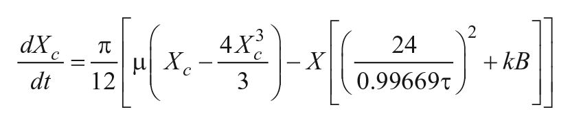
A mathematical model of the human circadian pacemaker developed by Forger and colleagues (1999) was used to perform all simulations. The model is a modified van der Pol oscillator that consists of Process P and Process L (Forger et al., 1999). Process P describes the oscillator representing the circadian pacemaker, and Process L represents the processing of external light and includes a phase-dependent sensitivity modulation. The equations associated with the 2 components of the model are as follows:

Process P

\frac{d X}{d t} = \frac{π}{12} (X_{c} + B)

\frac{d X_{c}}{d t} = \frac{π}{12} [μ (X_{c} - \frac{4 X_{c}^{3}}{3}) - X [{(\frac{24}{0.99669 τ})}^{2} + k B]]

Process L

α (I) = α_{0} (\frac{I^{p}}{I_{0}^{p}})

\frac{d n}{d t} = 60 [α (I) (1 - n) - β n]

\hat{B} = G (1 - n) α (I)

Sensitivity Modulation

B = \hat{B} (1 - s_{1} X) (1 - s_{2} X_{c}) .

External light, I(t), enters the system through equation $α (I)$ , which represents the drive rate. The variable $n$ models phototransduction, and both $n$ and $α (I)$ contribute to the output drive $\hat{B,}$ which then feeds into the sensitivity modulation $B$ . The sensitivity modulation dictates how light from Process L interacts with Process P, thereby introducing phase dependence into the light effect. In Process P, $X$ represents endogenous circadian body temperature and $X_{c}$ is a complementary variable. Therefore, minimums of $X$ correspond to minimum core body temperature ( $C B T_{m i n})$ , an experimental marker of circadian phase.

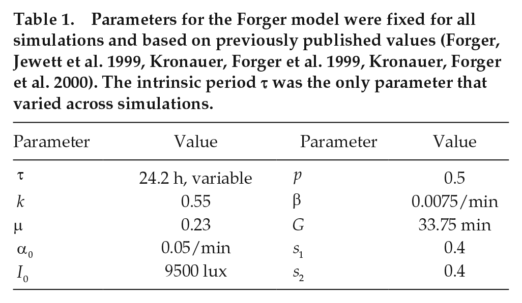
Kronauer and colleagues established baseline parameters of this circadian pacemaker model, including τ, $α_{0},$ and $β,$ by fitting the model to experimental data collected from healthy adults (Forger et al., 1999; Kronauer et al., 1999). The intrinsic circadian period, τ, represents the intrinsic period of the circadian oscillator in constant darkness. The model incorporates the effects of Aschoff’s rule on the circadian system such that the period of the oscillation decreases with increasing light exposure. Standard published parameter values (Forger et al., 1999; Kronauer et al., 1999; Kronauer et al., 2000), summarized in Table 1, were used for all simulations with the exception of the intrinsic period, τ, which was allowed to vary.

Table 1.

Parameters for the Forger model were fixed for all simulations and based on previously published values (Forger, Jewett et al. 1999, Kronauer, Forger et al. 1999, Kronauer, Forger et al. 2000). The intrinsic period τ was the only parameter that varied across simulations.

Parameter	Value	Parameter	Value
τ	24.2 h, variable	$p$	0.5
$k$	0.55	$β$	0.0075/min
$μ$ µ	0.23	$G$	33.75 min
$α_{0}$	0.05/min	$s_{1}$	0.4
$I_{0}$	9500 lux	$s_{2}$	0.4

Experimental Illuminance-Response Curve Protocol

The illuminance-response curve protocol design and the experimental data used as a test case for the method were previously published in a study by Zeitzer and colleagues (2000) designed to quantify the sensitivity of the human circadian pacemaker to nocturnal light. In this study, 23 healthy adults ages 18 to 44 years participated in the 9-day in-lab protocol. During the nocturnal light exposure, each participant was exposed to a different light intensity. Phase delay and percentage melatonin suppression were measured to construct illuminance-response curves of these measures.

The study protocol was as follows: for 2 weeks prior to the 9-day illuminance-response curve, protocol participants maintained a consistent 16:8 LD schedule (Fig. 1). Following 3 baseline days in the lab, they underwent an ~50-h constant routine at 15 lux in which the initial phase of the circadian system was assessed in the lab using minimum core body temperature ( $C B T_{m i n}$ ). Blood samples were taken every 30 min for plasma melatonin assay throughout the constant routine protocol. Study participants then experienced 8 h of darkness followed by 16 h of light centered about a 6.5-h light pulse. Each participant experienced a different light intensity ranging from 2.56 lux to 9106 lux. Individualized exact constant routine duration was chosen so that the light pulse began 6.75 h before predicted $C B T_{m i n}$ and ended 0.25 h before $C B T_{m i n}$ . The timing of light exposure was anchored to $C B T_{m i n}$ to control for the circadian phase of light exposure. During the remainder of the 16 h, the participants experienced dim light (<15 lux). Following another 8 h of darkness, they underwent a second ~30-h constant routine with blood sampling every 30 minutes for plasma melatonin assay to allow calculation of the phase shift in melatonin rhythm induced by the light exposure. Participants then slept for 8 h and were discharged upon waking on day 9.

Figure 1.

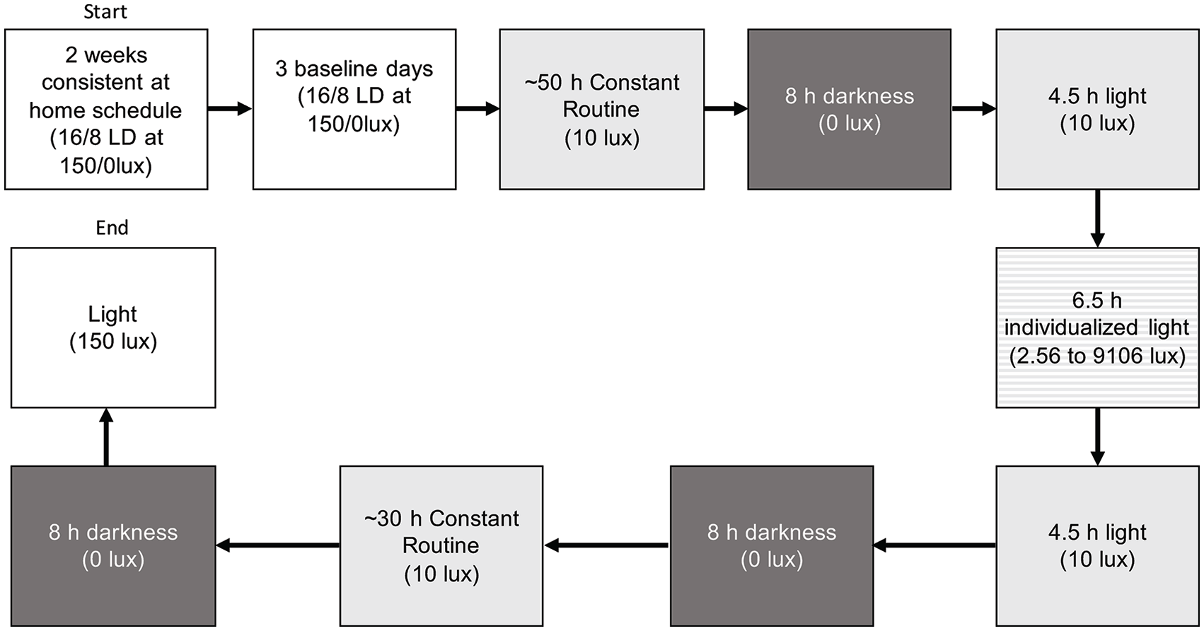
Schematic of the illuminance-response curve protocol with light intensities. Two weeks of a consistent schedule at home were followed by 3 baseline days in the lab. Then, participants underwent an ~50-h constant routine, an 8-h period of darkness, and a 16-h period of light. During the light period, the participants were exposed to a specific light intensity for 6.5 h (varied per person from 2.56 to 9106 lux). This exposure was timed to begin 6.75 h before CBT_min and to end 0.25 h before CBT_min to control for circadian phase. The remainder of the 16-h light period was spent in dim light. The light period was followed by 8 h of darkness, an ~30-h constant routine, and another 8 h of darkness to end the protocol.

Simulating the Experimental Illuminance-Response Curve Protocol

The simulated protocol was designed to mimic the experimental protocol described in the previous subsection. Before beginning the simulated illuminance-response curve protocol, the model simulated the circadian phase for 2 weeks on a consistent 16:8 h LD schedule with a light level of 150 lux from 0800 to 0000 h and a light level of 0 lux from 0000 to 0800 h. During the simulated in-lab portion of the protocol, light during the light period of the baseline days was set to 150 lux, dim light was set to 10 lux for the synthetic data and set to each participant’s measured light intensity (<15 lux) for experimental data, experimental light exposure was individualized and set to a light intensity ranging from 2.56 lux to 9106 lux, and dark periods were set to 0 lux (Fig. 1). To determine the appropriate duration of the constant routine in the simulated protocol, we first ran a preliminary simulation of the 2-week consistent schedule and a 56-h constant routine. Using these results, we determined $C B T_{m i n}$ and calculated the constant routine duration necessary to time the light pulse to begin 6.75 h before $C B T_{m i n}$ and end 0.25 h before $C B T_{m i n}$ . Using this newly calculated constant routine duration to ensure accurate timing of light exposure, we simulated the full protocol with appropriate nocturnal light exposure and computed light-induced phase shifts as the difference between $C B T_{m i n}$ during the first constant routine and $C B T_{m i n}$ during the second constant routine.

Model equations were implemented in MATLAB (Mathworks, Natick, MA) and solved numerically using the built-in MATLAB solver ode45 with a relative error tolerance of 1e-9 and an absolute error tolerance of 1e-10. The built-in MATLAB Signal Processing Toolbox function findpeaks was used to detect minima of $X$ to compute phase shifts.

MCMC Algorithm and Simulations

We implemented an MCMC method to estimate the representative intrinsic period, τ, for a given illuminance-response curve using the Metropolis algorithm. The goal of MCMC is to determine the posterior distribution, the probability of the parameter(s) given data $P (μ | D)$ , using Bayes’s theorem, which relates $P (μ | D)$ to the probability of the data given the parameters $P (D | μ)$ and the probability of the parameters $P (μ)$ :

P (μ | D) \propto P (D | μ) * P (μ)

The prior distribution, $P (μ),$ may include assumptions about what the distribution of the parameter(s) is likely to be. For the application of MCMC to illuminance-response data to determine representative intrinsic period τ, Bayes’s theorem relates intrinsic period to phase shifts as follows:

P (τ | P S) \propto P (τ | P S) * P (τ)

where $P S$ is a vector of phase shifts. Phase shift data ( $P S$ ) were simulated using the same light intensities as the experimental data. Each data point was assumed to be normally distributed with a mean of the measured phase shift and a 0.5-h standard deviation. This standard deviation was chosen to balance the percentage of accepted samples with the accuracy of the estimated representative intrinsic periods. The Metropolis algorithm was implemented in MATLAB and completed 10,000 iterations per MCMC run. The MCMC runs were started from different initial chain values (23.8, 24.1, and 24.7 h) to verify that the starting point of the chain did not affect the estimated distributions. All densities are presented with a 5% burn-in; that is, the first 500 iterations are not included in the analyses and metrics.

MCMC and Illuminance-Response Curve Test Cases

To validate the MCMC approach, we produced synthetic phase shift data sets using model simulations in which the generative single τ or multiple τ’s were known. Two different cases of synthetic data were considered. The first test case was the single τ illuminance-response curve, for which all data points on the illuminance-response curve were generated using one τ value. We simulated single τ illuminance-response curves for τ= 23.7, 24.2, 24.6, and 24.9 h. We also considered multi-τ illuminance-response curves where synthetic data were generated using a collection of 23 τ’s drawn from normal distributions with means of 23.7, 24.2, and 24.6 h and various standard deviations. The single τ illuminance-response curves represent an idealized case in which all phase shifts reflect the same τ. By contrast, the multi-τ illuminance-response curves are consistent with experimentally generated illuminance-response curves in which each point represents the phase shift of a different individual.

To generate synthetic data using known τ’s, the circadian pacemaker model simulated the experimental illuminance-response curve protocol across the range of light intensities. Phase shifts were calculated for each illuminance level and then used to specify the phase shift data for the Metropolis algorithm. The algorithm requires specifying a standard deviation for the data to account for potential error in the data from factors such as errors in melatonin assay, alignment of phase angle, and light intensity delivered. After experimenting with different standard deviations in the synthetic data, we determined that a standard deviation of 0.5 h balanced the percentage of accepted samples with good agreement between data and representative period. Therefore, a standard deviation of 0.5 h was used for all simulated phase shift data. For all runs with simulated illuminance-response curve data, the prior was selected to be $U (23.5, 25)$ to reflect the range of τ’s found for healthy adults (Smith et al., 2009; Duffy et al., 2011). After the algorithm completed 10,000 iterations, the known τ value or distribution was compared with the results from the algorithm with a 5% burn-in.

Using previously published light intensities and phase shifts (Zeitzer et al., 2000), we used this MCMC method to estimate the distribution of the representative intrinsic period of the group of 23 healthy adults who participated in the protocol. Each data point was assumed to be normally distributed with a mean set to the participant’s measured phase shift and a standard deviation of 0.5 h. This standard deviation was implemented based on results using the synthetic data as described above. We estimated the representative intrinsic period for this collection of experimental data using 2 different priors. We considered both a uniform prior ( $U (23.5, 25)$ ) that imposes minimal assumptions on the parameter τ, and, conversely, we considered a normal prior ( $N (24.2, {0.2}^{2})$ ) that assumes that the population τ is drawn from the established distribution of healthy adult intrinsic periods.

For all test cases, we completed 12 simulations consisting of 4 runs from each of the 3 initial chain values (23.8, 24.1, and 24.7 h). We averaged the estimated intrinsic period over all 12 simulations to obtain the representative τ value for the data set. In addition, we computed the standard deviation, the credible interval, and the percentage of accepted samples for each of the 12 MCMC runs.

The MCMC approach provides a flexible method for estimating representative intrinsic period; however, given the structure of the illuminance-response curve data, simpler regression approaches may also be used. To compare MCMC estimates to estimates obtained using other parameter estimation approaches, we implemented a standard minimization and regression method using 3 different cost functions. Additional details regarding this approach are available in the online supplementary material.

Results

Structure of Illuminance-Response Curve and τ’s

The structure of the simulated illuminance-response curve depends on τ. When the illuminance-response curves were simulated with different τ values, a stacked structure of curves was generated in which increasing τ values produced larger phase delays (negative phase shifts) compared with curves generated with smaller τ values (Fig. 2). In addition, these simulations illustrated the range of phase shift values that are produced by this model over the given range of τ values and light intensities. Although phase shifts are not unique functions of τ values and light intensities because of compensations between variables, the structure of the oscillator constrains the interactions between these parameters (Fig. 2B).

Figure 2.

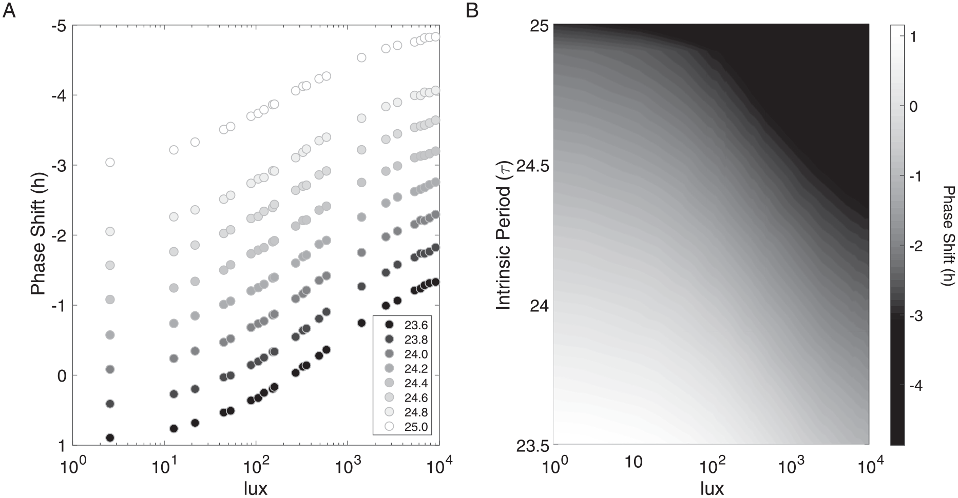
Illuminance-response curves depend on intrinsic period and light intensity. (A) Simulated illuminance-response curves show a stacked structure as intrinsic period τ is varied between 23.6 and 25.0 h. As τ increases over a physiological range, the shape of the illuminance-response curves is maintained, and the phase shift (h) values become more negative across light intensities. (B) Heat map of simulated phase shifts for light intensities and intrinsic periods (τ from 23.5 to 25.0 h) shows compensations between these variables. Light intensities were chosen to range from 1 to 10,000 lux, and interpolation was implemented to smooth the heat map.

Single τ Illuminance-Response Curves

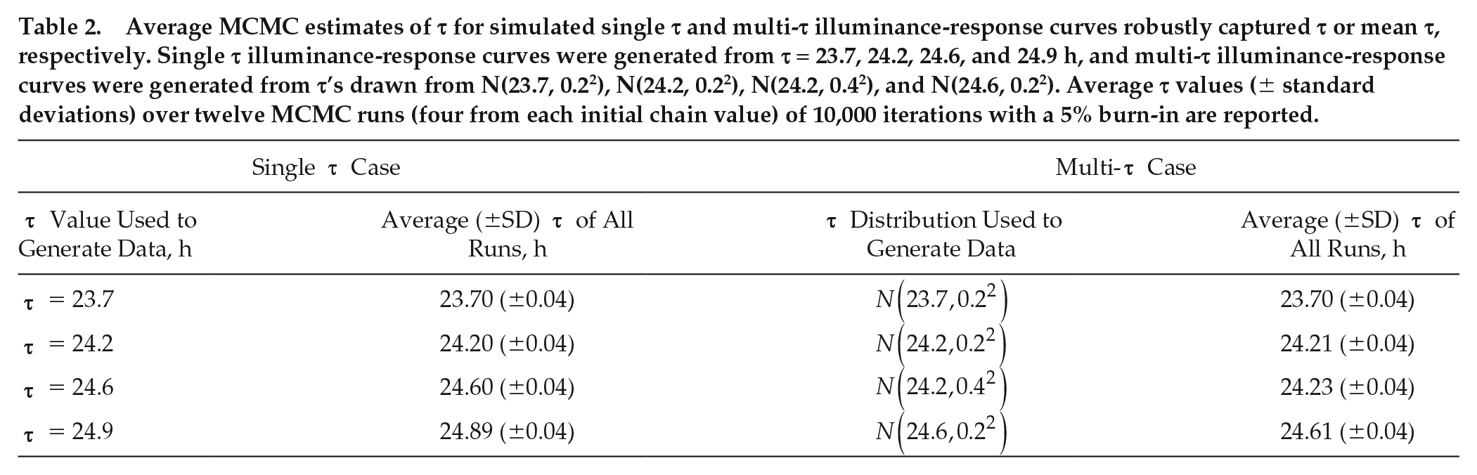
The application of the Metropolis algorithm to the simulated single τ illuminance-response curves produced representative τ values almost exactly equal to the τ value used to generate the single τ illuminance-response curve data. These curves were simulated with synthetic τ’s equal to 23.7, 24.2, 24.6, and 24.9 h, respectively. The posteriors were very similar to the sample means with agreement up to 2 significant figures for each estimated τ and standard deviations less than 0.05 h for all MCMC runs independent of initial chain value (Table 2; Suppl. Table S2). This agreement was also evident in the kernel densities, which generally overlapped for all 12 runs (Fig. 3). In addition, the means from individual runs and the means obtained by averaging over all 12 runs were within 0.01 of the τ value that was used to generate each phase shift data set, the credible intervals were less than 0.2 h, and the credible intervals contained the generative τ values (Suppl. Tables S2 and S3). The average percentage of accepted samples ranged from 41% to just more than 45% for all initial chain values and all data sets. Similar estimated intrinsic periods were obtained using standard optimization approaches (Suppl. Table S1).

Table 2.

Average MCMC estimates of τ for simulated single τ and multi-τ illuminance-response curves robustly captured τ or mean τ, respectively. Single τ illuminance-response curves were generated from τ = 23.7, 24.2, 24.6, and 24.9 h, and multi-τ illuminance-response curves were generated from τ’s drawn from N(23.7, 0.2²), N(24.2, 0.2²), N(24.2, 0.4²), and N(24.6, 0.2²). Average τ values (± standard deviations) over twelve MCMC runs (four from each initial chain value) of 10,000 iterations with a 5% burn-in are reported.

Single τ Case		Multi-τ Case
τ Value Used to Generate Data, h	Average (±SD) τ of All Runs, h	τ Distribution Used to Generate Data	Average (±SD) τ of All Runs, h
τ = 23.7	23.70 (±0.04)	$N (23.7, {0.2}^{2})$	23.70 (±0.04)
τ = 24.2	24.20 (±0.04)	$N (24.2, {0.2}^{2})$	24.21 (±0.04)
τ = 24.6	24.60 (±0.04)	$N (24.2, {0.4}^{2})$	24.23 (±0.04)
τ = 24.9	24.89 (±0.04)	$N (24.6, {0.2}^{2})$	24.61 (±0.04)

Figure 3.

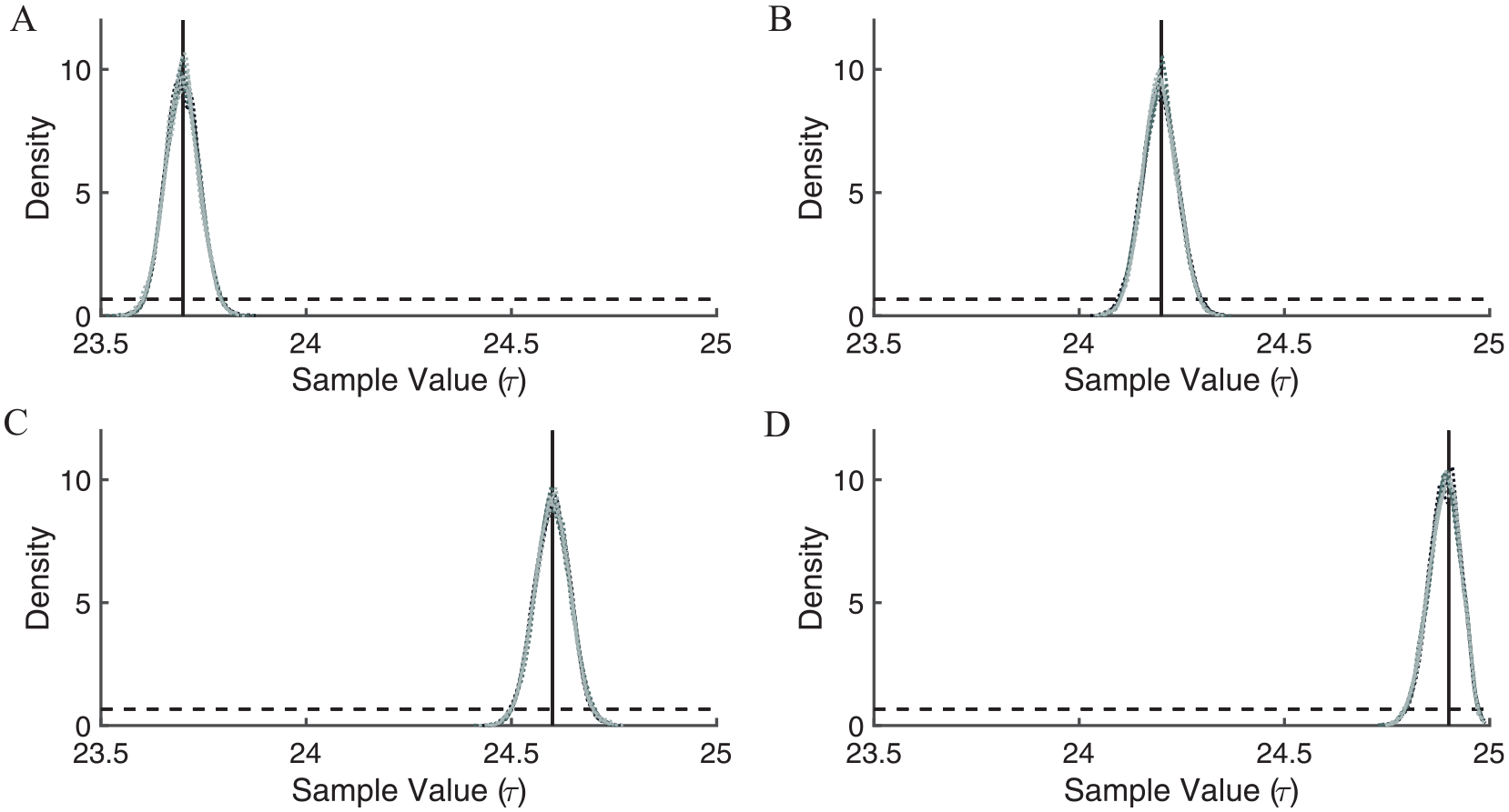
Kernel densities of 12 Markov-Chain Monte Carlo runs (4 from each initial chain value) reflect estimates of τ using synthetic single τ illuminance-response curve data, where τ = 23.7 (A), 24.2 (B), 24.6 (C), and 24.9 h (D). The 4 light-gray (initial chain value 23.8 h), 4 dark-gray (initial chain value 24.1 h), and 4 black (initial chain value 24.7 h) dotted lines indicate kernel densities. For each of the single τ illuminance-response curve data sets, the 12 kernel densities generally overlap because of the similarities among the posteriors across initial chain values. The black solid line indicates the known τ value with which the data were simulated. The black dashed line indicates the uniform prior.

Multi-τ Illuminance-Response Curves

Multi-τ illuminance-response curves were simulated with τ’s drawn from $N (23.7, {0.2}^{2})$ , $N (24.2, {0.2}^{2}),$ $N (24.2, {0.4}^{2})$ , and $N (24.6, {0.2}^{2})$ distributions. As with the single τ case, the estimated representative τ value obtained from the posterior distribution was almost exactly equal to the mean of the distribution from which the τ’s were drawn, even when the standard deviation in the data was increased. Over 12 runs with 3 initial chain values (4 runs per initial chain value), the posterior distributions were very similar to the sample means, agreeing up to 2 significant figures for each simulated data set with standard deviations less than 0.05 h (Suppl. Table S4). Similarly, we observed overlapping density plots of the kernel distributions of the runs, indicating close agreement of these distributions and minimal dependence on initial chain values (Fig. 4). Furthermore, the overall average means of all runs were within 0.02 h of the mean of the distribution of the τ’s for each data set and had small standard deviations (Table 2). The credible intervals generated from the runs were narrow and captured the means of the distributions used to generate the synthetic data (Suppl. Table S5). The average percentage of accepted samples ranged from 42% to 46% for all initial chain values and data sets. For the multi-τ illuminance-response curves, similar estimated intrinsic periods were obtained using regression approaches (Suppl. Table S1).

Figure 4.

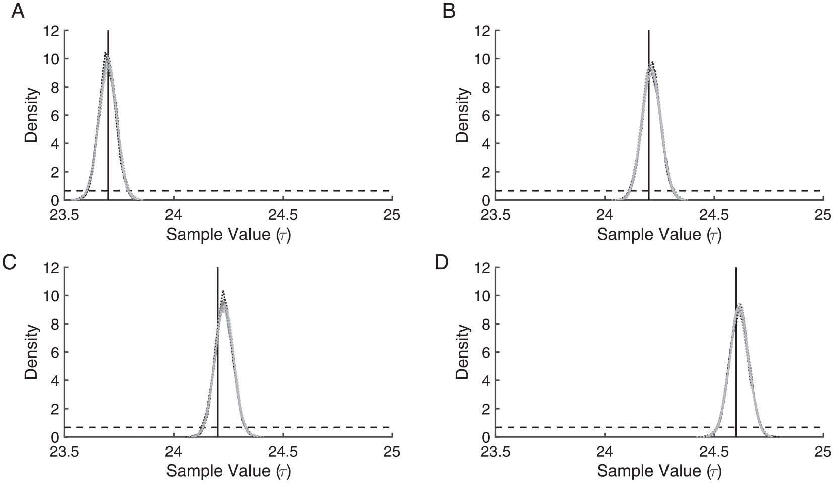
Kernel densities of 12 Markov-Chain Monte Carlo runs (4 from each initial chain value) reflect estimates of τ using synthetic multi-τ illuminance-response curve data, where τ’s were drawn from N(23.7, 0.2²) (A), N(24.2, 0.2²) (B), N(24.2, 0.4²) (C), and N(24.6, 0.2²) (D) distributions. The 4 light-gray (initial chain value 23.8 h), 4 dark-gray (initial chain value 24.1 h), and 4 black (initial chain value 24.7 h) dotted lines indicate kernel densities. For each of the multi-τ illuminance-response curve data sets, the 12 kernel densities generally overlap because of the similarities among the posteriors across initial chain values. The black solid line indicates the known mean τ value for the distribution from which the data were simulated. The black dashed line indicates the uniform prior.

Although this approach robustly identified the means of the distributions from which the τ’s were drawn to simulate the data, the standard deviations of the posterior distributions did not correspond to the standard deviations of these distributions. For example, when τ values were drawn from $N (24.2, {0.2}^{2})$ and $N (24.2, {0.4}^{2})$ distributions, respectively, the average standard deviations of the posteriors were nearly identical (Table 2; Suppl. S4), and the density plots were very similar (Fig. 4B, C). Therefore, although the mean of the posterior distribution provides a representative intrinsic period for the group of participants, the posterior distribution may not capture all of the variability present in the data.

Experimental Illuminance-Response Curve Data

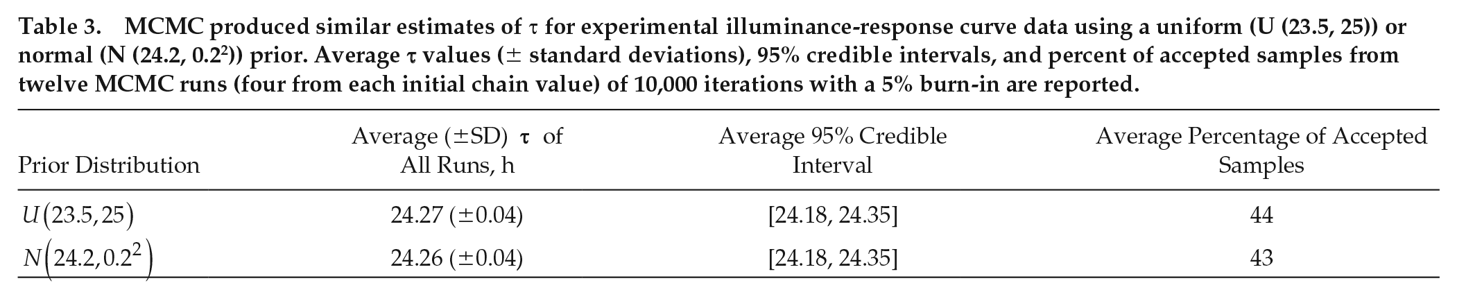
Applying MCMC to the experimental illuminance-response curve data resulted in estimates of representative intrinsic period that were close to the experimentally determined average healthy adult intrinsic period of 24.2 h independent of prior. With uniform priors, estimated mean τ values were 24.27 h for all runs and initial chain values (Table 3; Suppl. Table S6; Fig. 5). With normal priors, the estimated mean τ values were 24.26 h for all runs and initial chain values (Table 3; Suppl. Table S6; Fig. 5). All of the computed average 95% credible intervals contained 24.2 h (Table 3; Suppl. Table S7). The percentage of accepted samples was between 42.5% and 44.5% with the uniform prior and between 42% and 44% with the normal prior for all runs (Table 3). The density plots for the posterior distributions were very similar and did not depend on the choice of uniform or normal prior (Fig. 5). The illuminance-response curves generated with the representative intrinsic periods drawn from the posteriors determined using MCMC with either a uniform (Fig. 5B) or normal (Fig. 5D) prior provided good agreement with the experimentally determined illuminance-response curve although there was less variability in the simulated illuminance-response curves compared with the experimentally determined illuminance-response curve. Estimated intrinsic periods obtained using standard optimization approaches varied from the MCMC estimates based on the cost function used, but all estimates were within ±0.1 h of the estimates obtained using MCMC (Suppl. Table S1).

Table 3.

MCMC produced similar estimates of τ for experimental illuminance-response curve data using a uniform (U (23.5, 25)) or normal (N (24.2, 0.2²)) prior. Average τ values (± standard deviations), 95% credible intervals, and percent of accepted samples from twelve MCMC runs (four from each initial chain value) of 10,000 iterations with a 5% burn-in are reported.

Prior Distribution	Average (±SD) τ of All Runs, h	Average 95% Credible Interval	Average Percentage of Accepted Samples
$U (23.5, 25)$	24.27 (±0.04)	[24.18, 24.35]	44
$N (24.2, {0.2}^{2})$	24.26 (±0.04)	[24.18, 24.35]	43

Figure 5.

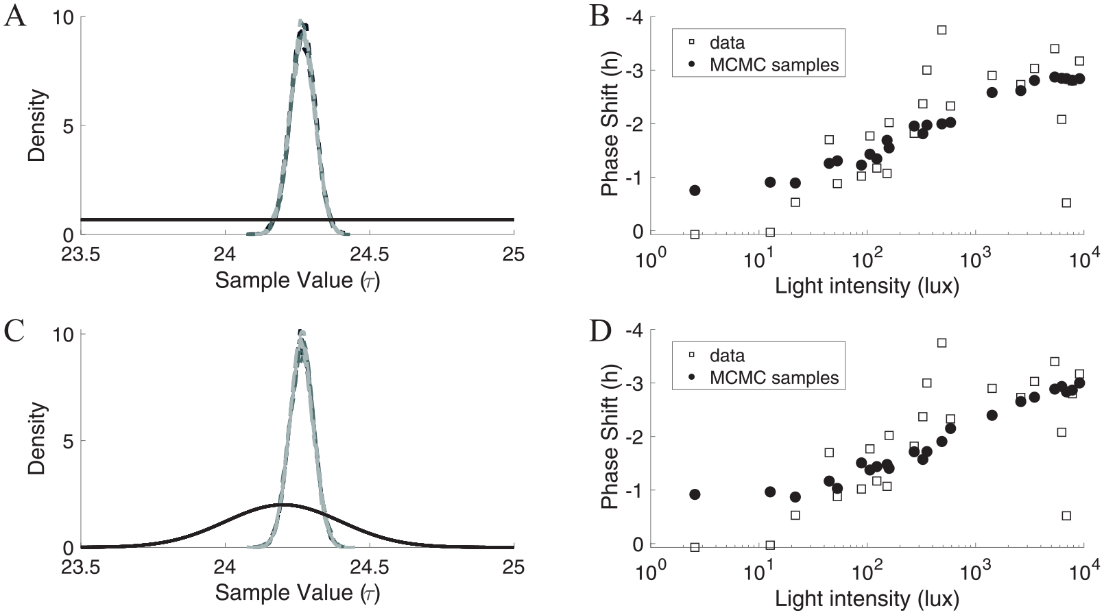
Estimating τ from human illuminance-response curve data using a uniform (U(23.5,25)) prior (A, B) or a normal (N(24.2, 0.2²)) prior (C, D) yielded similar results. (A) Kernel densities of 12 Markov-Chain Monte Carlo (MCMC) runs (4 from each initial chain value) to estimate τ using experimental illuminance-response curve data with a uniform prior indicated by the solid black line. The 4 light-gray (initial chain value 23.8 h), 4 dark-gray (initial chain value 24.1 h), and 4 black (initial chain value 24.7 h) dashed lines show the kernel densities. The curves generally overlap because of the similarities among the posteriors across initial chain values. (B) The experimental illuminance-response curve data (white squares) were well-approximated by the simulated illuminance-response curve data (black circles), although less variability was present in the simulated data. The simulated illuminance-response curve data were generated using τ values randomly sampled from the 12 posterior distributions generated using a uniform prior. (C) Kernel densities of 12 MCMC runs (4 from each initial chain value) to estimate τ using experimental illuminance-response curve data with a normal prior indicated by the solid black line. The 4 light-gray (initial chain value 23.8 h), 4 dark-gray (initial chain value 24.1 h), and 4 black (initial chain value 24.7 h) dashed lines show the kernel densities. The curves generally overlap because of the similarities among the posteriors across initial chain values. (D) The experimental illuminance-response curve data (white squares) were well-approximated by the simulated illuminance-response curve data (black circles), although less variability was present in the simulated data. The simulated illuminance-response curve data were generated using τ values randomly sampled from the 12 posterior distributions generated using a normal prior.

Discussion

Intrinsic Period Affects Simulated Illuminance-Response Curves

The intrinsic period of the circadian pacemaker, τ, affects the shape of illuminance-response curves simulated using distinct τ values, and this structure may be exploited to estimate a representative τ from illuminance-response curve data. As intrinsic period increases, the phase shifts become more negative across light intensities while maintaining a similar curve shape. Thus, there are distinct illuminance-response curves for each τ value with no intersections between curves. These features of illuminance-response curves associated with varying τ values demonstrate that this type of data is a good candidate for identifying τ using parameter estimation techniques. In practice, illuminance-response curves are generated using data from multiple participants and reflect each individual’s circadian features. It is important to interpret the estimated representative group intrinsic period in this context and to recognize that this approach does not provide information about an individual’s intrinsic period but instead identifies a representative intrinsic period for a group of study participants.

Illuminance-Response Curve Test Cases

We validated this methodology by applying the Metropolis algorithm to both single τ and multi-τ illuminance-response curve synthetic data sets. Simulated phase shift data were generated using a single τ value or collection of τ values drawn from a normal distribution. For both test cases, our method produced estimates of representative intrinsic period that were very close to the specified τ value or mean τ value, respectively. To facilitate comparisons between runs, we estimated τ with 6 significant figures. However, this is likely beyond the level of precision of τ estimates obtained experimentally using FD protocols (Czeisler et al., 1999). Notably, our estimates of representative group intrinsic period were obtained using an uninformative prior. Although a more informative prior may be preferable when a priori information about the parameters is available, our results suggest that it is not necessary to impose assumptions on the prior to obtain accurate estimates for this problem.

The MCMC implementation was robust with respect to a range of implementation metrics. Over multiple trials, estimates of representative intrinsic periods have average standard deviations of less than 0.05 h, narrow 95% credible intervals, and similar kernel density plots. There was no evidence in any of the metrics that the mean estimates of τ, were influenced by the initial chain value or assumptions on the prior. The average percentage of accepted samples was between 41% and 46%, an acceptable range for MCMC methods (Banerjee et al., 2003). Overall, these results support the applicability of MCMC methods to accurately estimate the representative intrinsic period of a group of study participants, given appropriate illuminance-response curve data.

Application to Experimental Data

When applied to the illuminance-response curve data from 23 healthy adult participants, this method predicted a representative intrinsic period consistent with the mean τ reported for this population (Czeisler et al., 1999). Specifically, the mean τ of 24.18 ± 0.04 h estimated in a healthy young adult population (Czeisler et al., 1999) is very close to the group τ of the illuminance-response curve study participants, which was estimated to be 24.27 or 24.26 h using uniform or normal priors, respectively. The similarity of these estimates of representative group τ suggests that, for these data, a relatively uninformative prior (like $U (23.5, 25)$ ) produces similar results compared with a more informative prior (like $N (24.2, {0.2}^{2})$ ). Therefore, as discussed in the context of the synthetic data, although a more informative prior may be preferable when a priori information about the parameters is available, our results suggest that an uninformative prior may be sufficient. This flexibility is an important feature for broader application of the method to illuminance-response data from study populations where there are no previous estimates of intrinsic circadian period.

As with the synthetic data, all metrics indicated that the MCMC implementation was robust. The mean estimates of representative τ percentage of accepted samples, and credible intervals were reasonable, were similar across runs, and were not affected by initial chain values. However, the estimates obtained with the MCMC approach were consistent with results obtained using standard parameter optimization methods. Overall, these results suggest that this method applied to illuminance-response curve data can be used to determine a reasonable estimate of the representative intrinsic period for a group of study participants.

Limitations

Mathematical models are powerful tools for interpreting data, making predictions, and informing experimental protocol design. However, models have underlying assumptions that may introduce model dependence in simulation results. The Forger circadian pacemaker model was selected for this study because it includes light processing, it has been fitted to healthy adult data, it has been widely used for many applications, and it includes τ as an explicit parameter. Furthermore, the model was calibrated using data from populations generally consistent with our study population. However, applications of this model to describe light sensitivity or other circadian features in demographic populations in which there is evidence for potential variation in multiple parameters may require multiple parameter estimates. For example, differences in light sensitivity may occur in early childhood (Higuchi et al., 2014), adolescence (Crowley et al., 2015), or with age (Duffy et al., 2007) and may alter Process L, thereby affecting the relationship between illuminance-response curve data and intrinsic circadian period. The flexibility to estimate multiple parameters given various circadian data types represents an advantage of the MCMC approach. In future work, a multiparameter MCMC approach could be used to investigate the relationship of multiple parameters (e.g., parameters affecting light sensitivity and intrinsic period) to illuminance-response curve data.

Although this method reliably detected the mean τ used to generate the multi-τ simulated illuminance-response curves, the standard deviations of the posterior distributions of τ did not reflect the standard deviations of the τ values used to generate the synthetic data. This result suggests that group τ estimates will be robust to individual outliers; however, it also indicates that the posterior distribution does not describe the variability of the intrinsic periods present within the participant group contributing to the illuminance-response curve data. Similarly, the illuminance-response curves simulated from posterior distributions derived from experimental data showed less variability compared with the experimentally determined illuminance-response curves. This aspect of the MCMC approach limits the interpretation of the representative τ for potentially heterogeneous populations. Recent work has highlighted interindividual differences in the sensitivity of the human circadian clock to evening light as measured by dose-response curves in melatonin suppression (Phillips et al., 2019), but less is known about interindividual differences in phase-shifting responses. Future work is needed to determine the interindividual variability present in phase shifts of the circadian clock in response to light exposure and the implications of this variability for illuminance-response curves constructed from ensemble data.

Conclusions and Implications

We have developed a method to estimate the representative intrinsic period, τ of a group of study participants using a mathematical model of the human circadian pacemaker, the Metropolis algorithm, and illuminance-response curve data. We have validated this method using synthetic data and implemented it to estimate representative intrinsic period from experimental data collected from healthy adults. Applying this approach to illuminance-response curve data from other populations, such as children or adults with circadian disorders, who are not good candidates for FD protocols, could contribute to understanding circadian properties in these populations. Furthermore, because illuminance-response curves collectively represent phase shifts from a group of individuals, this analysis yields novel insights about the representative intrinsic circadian period of a population using existing data that reflect other circadian features of the individuals. Future work could extend this approach to other types of circadian data including PRCs or phase of entrainment. Improved understanding of circadian properties of a population may facilitate interpretation of existing data and inform circadian-based interventions ranging from light therapy to school start times.

Supplemental Material

supplemental_material_rev_final – Supplemental material for Estimating Representative Group Intrinsic Circadian Period from Illuminance-Response Curve Data

Supplemental material, supplemental_material_rev_final for Estimating Representative Group Intrinsic Circadian Period from Illuminance-Response Curve Data by Nora Stack, Jamie M. Zeitzer, Charles Czeisler and Cecilia Diniz Behn in Journal of Biological Rhythms

Footnotes

Acknowledgements

The authors would like to thank Monique LeBourgeois for helpful discussions related to this research. This study was supported by the National Science Foundation grants DMS 1412571 and DMS 1853511 and the National Institutes of Health grant R01HD087707.

Authors’ Note

This work was performed at the Colorado School of Mines.

Conflict of Interest Statement

The authors have no potential conflicts of interest with respect to the research, authorship, and/or publication of this article.

ORCID iD

Cecilia Diniz Behn

Notes

References

Aschoff

(1960) Exogenous and endogenous components in circadian rhythms. Cold Spring Harb Symp Quant Biol 25:11-28.

Aschoff

Pohl

(1978) Phase relations between a circadian rhythm and its zeitgeber within the range of entrainment. Naturwissenschaften 65(2):80-84.

Banerjee

Carlin

Gelfand

(2003) Hierarchical modeling and analysis for spatial data. London: Chapman and Hall.

Belle

Diekman

Forger

Piggins

(2009) Daily electrical silencing in the mammalian circadian clock. Science 326(5950):281-284.

Bordyugov

Abraham

Granada

Rose

Imkeller

Kramer

Herzel

(2015) Tuning the phase of circadian entrainment. J R Soc Interface 12(108):20150282.

Burgess

Revell

Molina

Eastman

(2010) Human phase response curves to three days of daily melatonin: 0.5 mg versus 3.0 mg. J Clin Endocrinol Metab 95(7):3325-3331.

Buxton

Frank

L’Hermite-Baleriaux

Leproult

Turek

Van Cauter

(1997) Roles of intensity and duration of nocturnal exercise in causing phase delays of human circadian rhythms. Am J Physiol 273(3 Pt 1):E536-E542.

Carskadon

Acebo

Jenni

(2004) Regulation of adolescent sleep: implications for behavior. Ann N Y Acad Sci 1021:276-291.

Carskadon

Labyak

Acebo

Seifer

(1999) Intrinsic circadian period of adolescent humans measured in conditions of forced desynchrony. Neurosci Lett 260(2):129-132.

10.

Crowley

Cain

Burns

Acebo

Carskadon

(2015) Increased sensitivity of the circadian system to light in early/mid-puberty. J Clin Endocrinol Metab 100(11):4067-4073.

11.

Czeisler

Duffy

Shanahan

Brown

Mitchell

Rimmer

Ronda

Silva

Allan

Emens

, et al. (1999) Stability, precision, and near-24-hour period of the human circadian pacemaker. Science 284:2177-2181.

12.

Danner

Phillips

(2008) Adolescent sleep, school start times, and teen motor vehicle crashes. J Clin Sleep Med 4(6):533-535.

13.

Diekman

Bose

(2018) Reentrainment of the circadian pacemaker during jet lag: east-west asymmetry and the effects of north-south travel. J Theor Biol 437:261-285.

14.

Duffy

Cain

Chang

Phillips

Munch

Gronfier

Wyatt

Dijk

Wright

Jr. Czeisler

(2011) Sex difference in the near-24-hour intrinsic period of the human circadian timing system. Proc Natl Acad Sci U S A 108(Suppl 3):15602-15608.

15.

Duffy

Zeitzer

Czeisler

(2007) Decreased sensitivity to phase-delaying effects of moderate intensity light in older subjects. Neurobiol Aging 28(5):799-807.

16.

Dunster

de la Iglesia

Ben-Hamo

Nave

Fleischer

Panda

de la Iglesia

(2018) Sleepmore in Seattle: later school start times are associated with more sleep and better performance in high school students. Sci Adv 4(12):eaau6200.

17.

Eastman

Molina

Dziepak

Smith

(2012) Blacks (African Americans) have shorter free-running circadian periods than whites (Caucasian Americans). Chronobiol Int 29(8):1072-1077.

18.

Eastman

Suh

Tomaka

Crowley

(2015) Circadian rhythm phase shifts and endogenous free-running circadian period differ between African-Americans and European-Americans. Sci Rep 5:8381.

19.

Eastman

Tomaka

Crowley

(2016) Circadian rhythms of European and African-Americans after a large delay of sleep as in jet lag and night work. Sci Rep 6:36716.

20.

Fleshner

Booth

Forger

Diniz Behn

(2011) Circadian regulation of sleep-wake behaviour in nocturnal rats requires multiple signals from suprachiasmatic nucleus. Philos Trans A Math Phys Eng Sci 369(1952):3855-3883.

21.

Forger

Jewett

Kronauer

(1999) A simpler model of the human circadian pacemaker. J Biol Rhythms 14(6):532-537.

22.

Gooley

(2008) Treatment of circadian rhythm sleep disorders with light. Ann Acad Med Singapore 37(8):669-676.

23.

Granada

Bordyugov

Kramer

Herzel

(2013) Human chronotypes from a theoretical perspective. PLoS One 8(3):e59464.

24.

Higuchi

Nagafuchi

Lee

Harada

(2014) Influence of light at night on melatonin suppression in children. J Clin Endocrinol Metab 99(9):3298-3303.

25.

Khalsa

Jewett

Cajochen

Czeisler

(2003) A phase response curve to single bright light pulses in human subjects. J Physiol 549(Pt 3):945-952.

26.

Klerman

Dijk

Kronauer

Czeisler

(1996) Simulations of light effects on the human circadian pacemaker: implications for assessment of intrinsic period. Am J Physiol 270(1 Pt 2):R271-R282.

27.

Kronauer

Forger

Jewett

(2000) Errata: quantifying human circadian pacemaker response to brief, extended, and repeated light stimuli over the photopic ranges. J Biol Rhythms 15(2):184-186.

28.

Kronauer

Forger

Jewett

(1999) Quantifying human circadian pacemaker response to brief, extended, and repeated light stimuli over the phototopic range. J Biol Rhythms 14(6):500-515.

29.

Landrigan

Czeisler

Barger

Ayas

Rothschild

Lockley

, Harvard Work Hours, Health and Safety Group (2007) Effective implementation of work-hour limits and systemic improvements. Jt Comm J Qual Patient Saf 33(11 suppl):19-29.

30.

Lewy

Bauer

Ahmed

Thomas

Cutler

Singer

Moffit

Sack

(1998) The human phase response curve (PRC) to melatonin is about 12 hours out of phase with the PRC to light. Chronobiol Int 15(1):71-83.

31.

Minors

Waterhouse

Wirz-Justice

(1991) A human phase-response curve to light. Neurosci Lett 133(1):36-40.

32.

Phillips

Chen

Robinson

(2010) Probing the mechanisms of chronotype using quantitative modeling. J Biol Rhythms 25(3):217-227.

33.

Phillips

AJK

Vidafar

Burns

McGlashan

Anderson

Rajaratnam

SMW

Lockley

Cain

(2019) High sensitivity and interindividual variability in the response of the human circadian system to evening light. Proc Natl Acad Sci U S A 116(24):12019-12024.

34.

Revell

Molina

Eastman

(2012) Human phase response curve to intermittent blue light using a commercially available device. J Physiol 590(19):4859-4868.

35.

Roenneberg

Wirz-Justice

Merrow

(2003) Life between clocks: daily temporal patterns of human chronotypes. J Biol Rhythms 18(1):80-90.

36.

Saper

Scammell

(2005) Hypothalamic regulation of sleep and circadian rhythms. Nature 437(7063):1257-1263.

37.

Smith

Burgess

Fogg

Eastman

(2009) Racial differences in the human endogenous circadian period. PLoS One 4(6):e6014.

38.

Stack

Barker

Carskadon

Diniz Behn

(2017) A model-based approach to optimizing ultradian forced desynchrony protocols for human circadian research. J Biol Rhythms 32(5):485-498.

39.

Welsh

Takahashi

Kay

(2010) Suprachiasmatic nucleus: cell autonomy and network properties. Annu Rev Physiol 72:551-577.

40.

Wright

Jr. Gronfier

Duffy

Czeisler

(2005) Intrinsic period and light intensity determine the phase relationship between melatonin and sleep in humans. J Biol Rhythms 20(2):168-177.

41.

Zeitzer

Dijk

Kronauer

Brown

Czeisler

(2000) Sensitivity of the human circadian pacemaker to nocturnal light: melatonin phase resetting and suppression. J Physiol 26(Pt 3):695-702.

Supplementary Material

Please find the following supplemental material available below.

For Open Access articles published under a Creative Commons License, all supplemental material carries the same license as the article it is associated with.

For non-Open Access articles published, all supplemental material carries a non-exclusive license, and permission requests for re-use of supplemental material or any part of supplemental material shall be sent directly to the copyright owner as specified in the copyright notice associated with the article.

0.00 MB

0.21 MB