Sage Journals: Discover world-class research

Abstract

While circadian rhythms in physiology and behavior demonstrate remarkable day-to-day precision, they are also able to exhibit plasticity in a variety of parameters and under a variety of conditions. After-effects are one type of plasticity in which exposure to non–24-h light-dark cycles (T-cycles) will alter the animal’s free-running rhythm in subsequent constant conditions. We use a mathematical model to explore whether the concept of synaptic plasticity can explain the observation of after-effects. In this model, the SCN is composed of a set of individual oscillators randomly selected from a normally distributed population. Each cell receives input from a defined set of oscillators, and the overall period of a cell is a weighted average of its own period and that of its inputs. The influence that an input has on its target’s period is determined by the proximity of the input cell’s period to the imposed T-cycle period, such that cells with periods near T will have greater influence. Such an arrangement is able to duplicate the phenomenon of after-effects, with relatively few inputs per cell (~4-5) being required. When the variability of periods between oscillators is low, the system is quite robust and results in minimal after-effects, while systems with greater between-cell variability exhibit greater magnitude after-effects. T-cycles that produce maximal after-effects have periods within ~2.5 to 3 h of the population period. Overall, this model demonstrates that synaptic plasticity in the SCN network could contribute to plasticity of the circadian period.

Keywords

plasticity period computational model after-effects mammal

Circadian rhythms in physiology and behavior demonstrate remarkable precision, with the standard error of the circadian period often less than 2 min per day (Pittendrigh, 1960; Pittendrigh and Daan, 1976). Yet the circadian system also exhibits the capacity for plasticity in a variety of parameters and under a variety of conditions. For instance, the duration of the active and rest phases (α and ρ, respectively) becomes shorter or longer with changing photoperiods. The circadian period (τ) is also highly plastic. Pittendrigh (1960) identified 3 situations leading to after-effects on τ. The first situation occurs when animals are housed under non–24-h cycles before being placed into constant darkness. Animals subjected to cycles with periods less than 24 h will exhibit shorter τs, while those exposed to cycles with periods greater than 24 h will exhibit longer τs (e.g., Aton et al., 2004; Azzi et al., 2014; Azzi et al., 2017; Boulos et al., 2002; Pittendrigh, 1960; Pittendrigh and Daan, 1976). The second situation identified by Pittendrigh (1960) is exposure to constant light. In nocturnal animals, constant light lengthens τ. Pittendrigh (1960) pointed out that this long τ persists when the organism is then placed into constant darkness. The third case of after-effects that Pittendrigh highlighted was that a single application of a zeitgeber in constant conditions could alter τ (Pittendrigh, 1960). This is true of both photic (Pittendrigh and Daan, 1976) and nonphotic (Weisgerber et al., 1997) zeitgebers. Pittendrigh later added a fourth type of after-effect, whereby photoperiod not only alters α and ρ, but also subsequent τ in constant conditions (Pittendrigh, 1964). In some cases, exposure to long days and short nights led to a shorter τ in subsequent constant darkness than was observed following short days and long nights (Pittendrigh, 1964), while in other cases, the opposite was observed (Pittendrigh and Daan, 1976).

The circadian clock is composed of thousands of cell-autonomous oscillators (Antle and Silver, 2005). These individual oscillators exhibit a range of periods (Herzog et al., 1998; Liu et al., 1997; Welsh et al., 1995) but must be coordinated to yield a dominant tissue-level period (Antle et al., 2003; Antle et al., 2007; Liu et al., 1997). Plasticity in α, ρ, and circadian amplitude under different photoperiods is due to the phase dispersion of individual oscillators (Meijer et al., 2010; Rohling et al., 2006; Schaap et al., 2003; VanderLeest et al., 2007). The mechanism by which after-effects on τ are mediated is less clear. Some have modeled after-effects on τ through examining phase (Beersma et al., 2017; Bordyugov and Herzel, 2014), while others have explored epigenetic contributions (Azzi et al., 2014; Azzi et al., 2017). Given the heterogeneity of periods of individual cells, and the necessity that these periods must be altered to yield a dominant tissue-level period, we wanted to explore how a network that exhibited synaptic plasticity might contribute to the after-effects observed after exposure to non–24-h T-cycles.

The concept of synaptic plasticity was initially proposed by Hebb (1949). Cells that play a role in consistently activating their targets undergo plasticity to strengthen their connection to their targets, while those whose activity rarely participates in activating the target are weakened. More enduring long-term changes are likely mediated by synaptic and dendritic rearrangement that strengthens (or weakens) the contribution of an afferent cell onto its targets (Agnihotri et al., 1998; Bailey et al., 2000; Bernardinelli et al., 2014; Forrest et al., 2018). Given the distribution of intrinsic periods in individual SCN cells, we theorize that cells with periods similar to that of an imposed T-cycle will experience synaptic potentiation such that they gain influence in the circadian network, while those with periods quite different from the imposed T-cycle will undergo synaptic depression, diminishing their contribution to the circadian network.

In this model, we conceive of the SCN as a population of individual oscillators with normally distributed periods. The period of each individual oscillator is a function of its own intrinsic period and a weighted average of the periods of its afferent cells, and the period of the whole system is simply the mean period from all of the oscillators in the ensemble. When exposed to a T-cycle, cells with intrinsic periods close to the imposed T-cycle become more dominant in the network, thereby having a greater influence over their efferent cells than oscillators with periods farther from the imposed T-cycle.

Materials And Methods

Model

Simulations were programmed using Python (3.7.0, Python.org). The software to run these simulations is available at https://dataverse.scholarsportal.info/dataset.xhtml?persistentId=doi:10.5683/SP2/ZX0KGH. Data were exported to Microsoft Excel for analysis and graphing. The SCN was conceived of as a population of oscillators with normally distributed free-running periods defined by a population mean (τ_pop) and standard deviation (σ_pop). While these variables can be manipulated, in most simulations, σ_pop was 1.2 h, based on the standard deviation of individual SCN cells in dispersed culture (Herzog et al., 1998; Liu et al., 1997; Welsh et al., 1995), and τ_pop was 24 h. From this population, a number of oscillators (N_osc) were randomly selected. N_osc was set to 100 unless otherwise specified. These individual oscillators were conceived of as an interconnected network, wherein each oscillator received a specified number of inputs (N_in), as depicted in Figure 1. N_in was set to 5 unless otherwise specified. These N_in connections were randomly assigned for each oscillator and were selected from the N_osc. No constraints were placed on this random assignment, so occasionally an oscillator would self-innervate or could receive multiple inputs from a particular oscillator. The oscillators that provided input to each oscillator were fixed throughout the simulation. The overall period of the system τ_sys was simply calculated as the mean of the periods of the individual oscillators τ_i that made up the system. This approach is similar to that suggested by Liu and colleagues (1997), as they observed that the free-running periods of behavioral rhythms were approximately equal to the mean of the periods of dispersed cells in culture.

Figure 1.

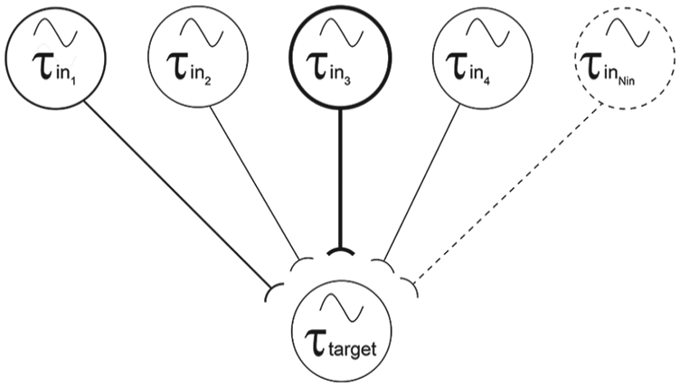
Every oscillator receives inputs from N_in other oscillators. The period of the target oscillator (τ_target) is modified by its inputs, such that its new period is a function of its original period and the influence-weighted periods of its inputs. Afferent cells with periods close to the imposed T-cycle (i.e., τ_in3 in this figure) will have greater influence on the target cell’s new period than cells with periods quite different from that of the imposed T-cycle (i.e., τ_inNin in this figure).

To model the influence of a T-cycle (T) on the period of the system, we conceived that the period of each oscillator could be modified by its inputs. The influence (Inf) that each input would have was proportional to how close its τ was to T according to equation 1 and Figure 2.

I n f = A \cdot e^{- \frac{{(τ_{i} - T)}^{2}}{2 {σ_{i n f}}^{2}}}

(1)

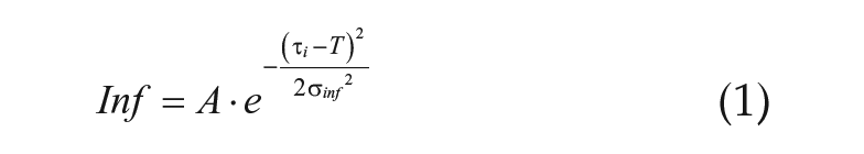
This equation creates a bell curve around T, such that oscillators with periods close to the imposed T-cycle would have the greatest influence, while those with periods quite different from T would have little influence. The width of the bell curve is defined by σ_inf and was set to 1 unless otherwise specified. The bell curve also had a scaling factor (A) that determined its height. A was set to 0.1 in all simulations unless otherwise specified. To determine the effect that an oscillator would have on its targets (τ_target), a period modifier was calculated according to equation 2.

M o d_{i n} = (I n f_{i n} \cdot t_{i n}) + t_{t a r g e t}

(2)

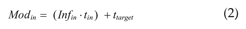
This modifier pulls τ_target toward its own period. To do this, the Inf_in variable was assigned a negative value if τ_in < τ_target and a positive value if τ_in > τ_target.

Figure 2.

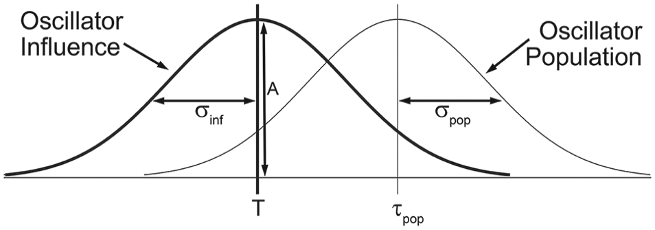
Oscillators in our model are randomly selected from a normally distributed population with a mean period of τ_pop and a standard deviation of σ_pop. The overall influence of each oscillator was calculated based on a normal distribution curve centered around the period of the imposed T-cycle (T). This curve had a specified width (σ_inf) and height (A). Each oscillator’s influence was dynamic and was recalculated with each iteration of the model as each oscillator’s period changed from cycle to cycle.

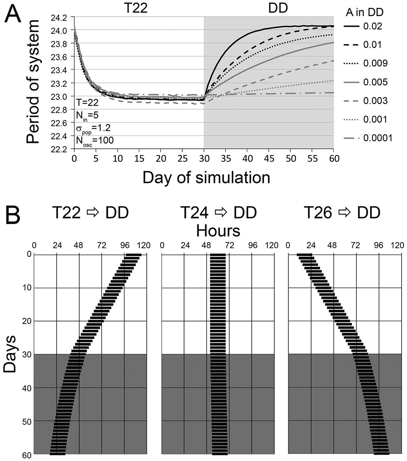
The period of each oscillator was recalculated each “day” based on its own period (τ_target) and the modifiers (Mod_in) from its N_in inputs, according to equation 3.

τ_{t a r g e t'} = \frac{τ_{t a r g e t} + \sum_{i = 1}^{N_{i n}} M o d_{i n_{i}}}{N_{i n} + 1}

(3)

This τ_target′ became the new τ_target for the subsequent “day.” This process was repeated in an iterative fashion, with each iteration representing another day under the imposed T-cycle. The overall period of the system τ_sys was calculated after each iteration.

Standard Simulations

The influence of a number of variables was explored. Each simulation was run 10 times, and the average response was recorded. Variables explored included the period of the T-cycle (T), the number of oscillators in the system (N_osc), the number of connections each oscillator received (N_in), the standard deviation of the population from which the oscillators were selected (σ_pop), and the height and width of the influence function (A and σ_inf).

T-cycle to DD Simulations

To simulate moving an animal into DD following T-cycle exposure, after 30 days, equation 1 was changed to Inf = A, where A was a value between 0.02 and 0.0001. This generated a flat influence function wherein no cell was more influential than another. The simulations were allowed to run for 30 more days in this state.

In Vivo to In Vitro Simulations

Three studies explored the after-effects of mice exposed to a T-cycle in vivo and then subsequently measured the period of their circadian systems in vitro using a transgenic luciferase reporter (Aton et al., 2004; Azzi et al., 2017; Molyneux et al., 2008). In each case, the period in vitro was negatively correlated with the period observed in vivo. Specifically, short T-cycles shortened the free-running periods in DD in vivo but led to longer free-running periods of luciferase rhythms in vitro. Conversely, long T-cycles lengthened the free-running periods in DD in vivo but led to shorter free-running periods of luciferase rhythms in vitro. To explore what would be needed to replicate these observations with our model, we made 2 hypotheses: (1) when SCN cultures are prepared, not all SCN neurons survive, and (2) the cells that are most sensitive to death are the ones that play the most prominent role in the network. This last assumption is analogous to what happens with cortical cells during an ischemic event. Strong cells in a network receive and produce many connections. During ischemic events, when one of these cells dies, it releases massive quantities of neurotransmitters, leading to excessive depolarization of its targets, thus causing an excitotoxic cascade that leads to secondary cell death in its postsynaptic targets (Szydlowska and Tymianski, 2010). Weaker cells in the network receive and produce relatively fewer connections. This would somewhat protect them from secondary cell death, since they receive fewer inputs and thus experience less depolarization. To model this, we set a threshold for Inf, such that oscillators with an influence above a critical value would be eliminated, while those with an influence below this threshold would survive. As parameters in our typical simulations lead to systems with little variability, weaker parameters (A = 0.05, σ_inf = 0.6, N_in = 4) and less iteration (10 days) were employed. The threshold for Inf = 0.015, so any oscillator with an Inf greater than this was eliminated from the system after the last iteration.

Results

Initial Simulations

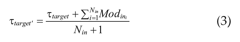
We initially explored how our system would respond to a range of T-cycles between 18 and 30 h (Fig. 3). For these initial simulations, we used a population of 100 oscillators randomly selected from a normally distributed population with a mean period of 24 ± 1.2 h. Each oscillator received inputs from 5 randomly selected oscillators from the initial 100. Each input oscillator was given an influence weight based the proximity of its period to the imposed T-cycle as specified in equation 1, with A = 0.1 and σ_inf = 1. The period of the target oscillator was modified according to equations 2 and 3. This new period for each oscillator was then used for the subsequent iteration of the simulation. The 5 specific oscillators that provided input to each target oscillator were kept stable throughout. The period of the system was calculated by averaging the periods of all 100 oscillators after each iteration of the simulation, and the simulation was run for 30 iterations. The simulation was run a total of 10 times, and the overall output was averaged. The largest responses were observed with T-cycles of 21.5 h on the low end and 26.5 h on the high end (Fig. 3B). T-cycles of 21 h and 27 h eventually yielded a system with similar periods to those with 21.5 h and 26.5 h T-cycles, but T21 and T27 influenced the system much more slowly, reaching this peak response after about 25 iterations, whereas the T21.5 and T26.5 neared their asymptote in only 10 to 15 iterations (Fig. 3A). T-cycles of 19 to 20 h and 28 to 29 h had diminished effects, and T-cycles of 18 h and 30 h left the system essentially unchanged from baseline.

Figure 3.

After-effects were produced over a wide range of T-cycles. (A) The average period of the system was calculated after each iteration of the model. Each trace represents the mean period from 10 separate simulations. Each simulation was based on 100 oscillators randomly selected from a normally distributed population with a mean period of 24 h and a standard deviation (σ_pop) of 1.2 h. T-cycle periods were tested between 18 and 30 h. (B) Periods (±standard deviations) after the final cycle plotted versus the period of the imposed T-cycle. Maximal after-effects were elicited with T-cycle periods of 21 to 21.5 h and 26.5 to 27 h.

Exploring Variability

To explore how our model influenced the variability of the populations, we focused on T-cycles of 22 h and 26 h. Variability between simulations was quite small (Fig. 4A), with standard deviations of <0.19 h. Variability was larger for T-cycles that pushed the limits of the system (e.g., T27 and T28, where the standard deviations were 0.28 h and 0.26 h, respectively; Fig. 3B).

Figure 4.

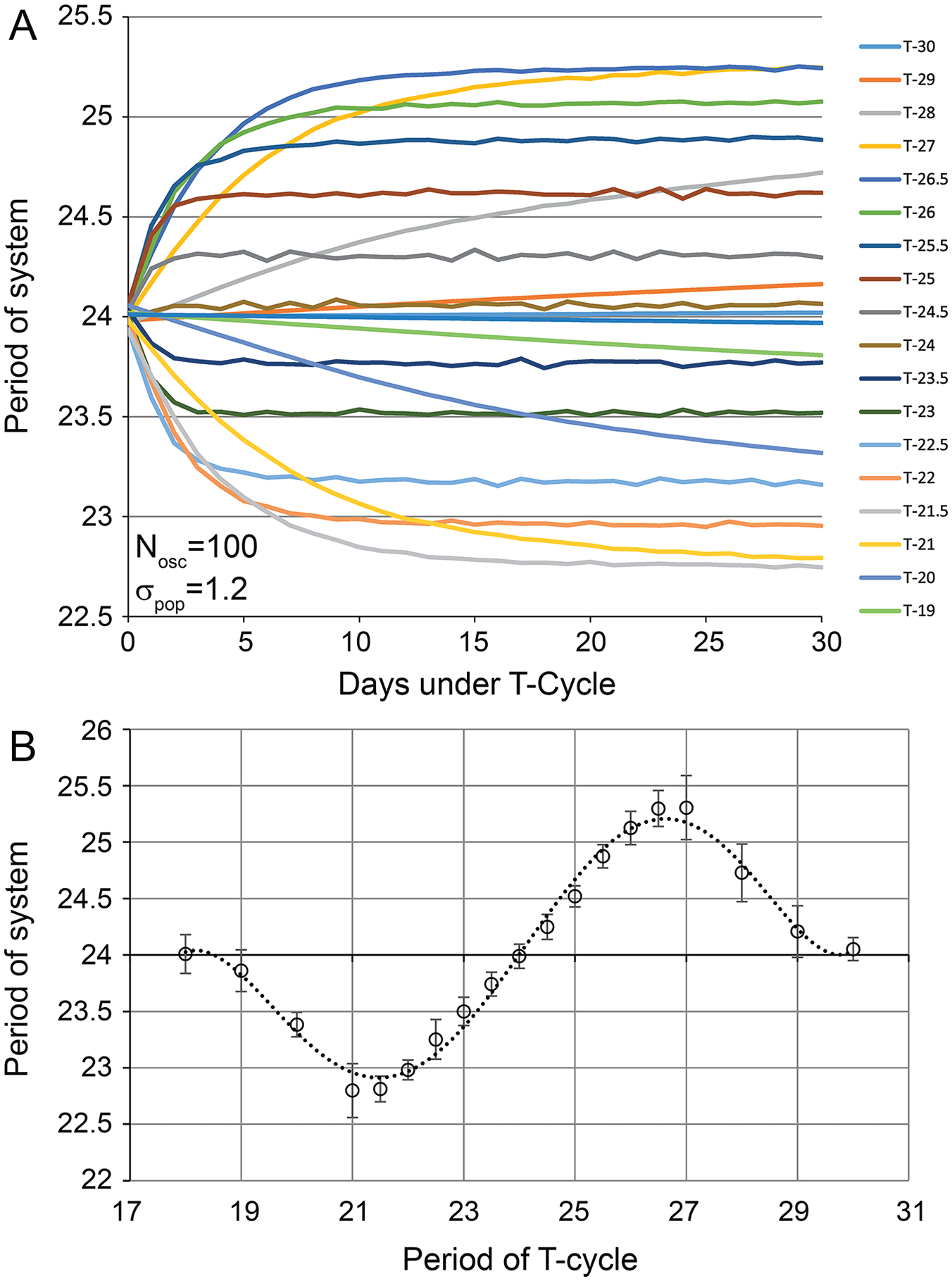
Exploring variance in the model. (A) Simulations were quite similar between replicates, yielding low variance. The average periods (±standard deviation) of each cycle from 10 simulations are presented for T22 (black circles) and T26 (gray circles). (B) Variance within simulations was also explored. Representative outputs from a single simulation for both T22 (black circles) and T26 (gray circles) were explored. Variance within the population quickly decreased from about the defined level of 1.2 h prior to the first iteration of the model to about 0.7 h around day 5. (C-G) Histograms of the periods of the oscillators in the representative simulations presented in B (T22 in black and T26 in gray) from days 0, 2, 5, 15, and 30. (C) On day 0 prior to application of the model, the populations of oscillators were very similar. (D) Within 2 days of application of the model, the populations started to diverge toward the period of their imposed T-cycles. (E) By day 5, the populations largely resembled their final distributions observed by day 15 (F) and 30 (G).

Within a simulation, the model quickly decreased the variability of the population of oscillators from its initial defined value near 1.2 h to near 0.64 h by about the 10th cycle (Fig. 4B). Starting from similar initial populations (Fig. 4C), T22 and T26 start to organize distinct clusters of oscillators that have lower variability even by day 2 (Fig. 4D). By day 5 (Fig. 4E), the population of oscillators largely resembles that observed at the midpoint (Fig. 4F) and final stages of the simulations (Fig. 4G).

T-cycle to DD Simulations

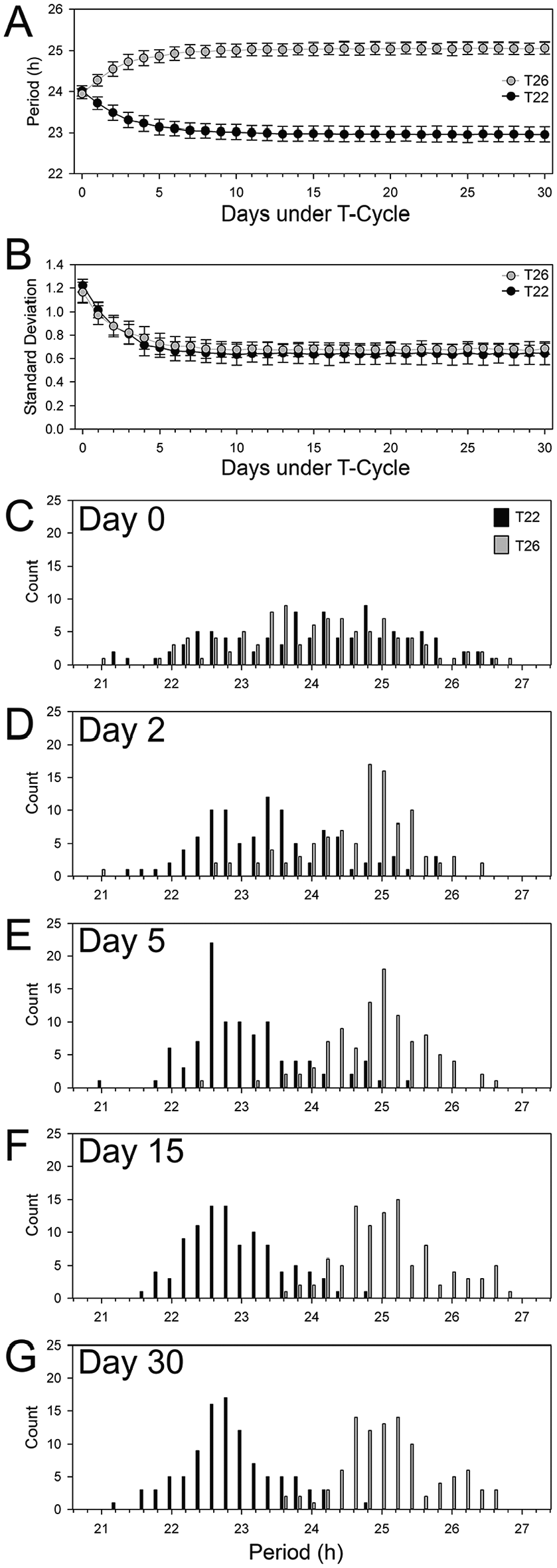
To explore how the system would evolve in DD after exposure to a T-cycle, we ran simulations for T22 and T26 as described above for 30 cycles. After these first 30 days, the influence function (equation 1) was changed to Inf = A with A set to a value between 0.02 and 0.0001, thus generating a horizontal line. In this manner, no oscillator was any more influential than any other. The simulation then continued for another 30 cycles. As A became larger, the system regressed to 24 h more quickly (Fig. 5A). Using the values from A = 0.001, we created actograms (Fig. 5B) for T22, T24, and T26, with the initial period set at that for the T-cycle and the subsequent output evolving in DD. For T22, the period on day 1 of DD was 22.88 h and increased to a period of 23.53 h by day 30 in DD. For T26, the period on day 1 of DD was 25.11 h and decreased to a period of 24.52 h by day 30 in DD.

Figure 5.

(A) Simulations exploring the effects of DD after T-cycle application. On day 30, the influence curve depicted in Figure 2 is changed to a flat horizontal line with a height of A. Values of A between 0.02 and 0.0001 were explored. The larger A, the more quickly the system relaxed back to near the original period of 24 h. For small values of A, the system’s period remained close to its final period on the last day of the T-cycle. (B) Actogram depictions of after-effects from our model. For the first 30 days, activity bouts (depicted by black rectangles) were plotted with the period of the imposed T-cycle (i.e., 22 h on the left, 24 h in the middle, and 26 h on the right). After 30 iterations of the model, the simulations were altered to use the influence function used in the above panel for A = 0.001 to determine the period on each of the following 30 days to plot the new free-running period of the ensemble in constant darkness (DD). After-effects that are intermediate to the original τ_pop (24 h in these cases) and the imposed T-cycles are apparent.

Oscillator Population Parameters

The initial parameters were selected arbitrarily for population size and number of inputs, and the standard deviation of the population was based on that observed for dispersed cells in vitro (Welsh et al., 1995). We next explored how systems would respond if we modified these variables individually while keeping the T-cycle consistent at 22 h. Population size (Fig. 6A) had no noticeable effect on the output of the simulation at all, with similar results being observed with populations as small as 50 oscillators and as large as 1000 oscillators. The only qualitative difference was that larger populations yielded smoother curves.

Figure 6.

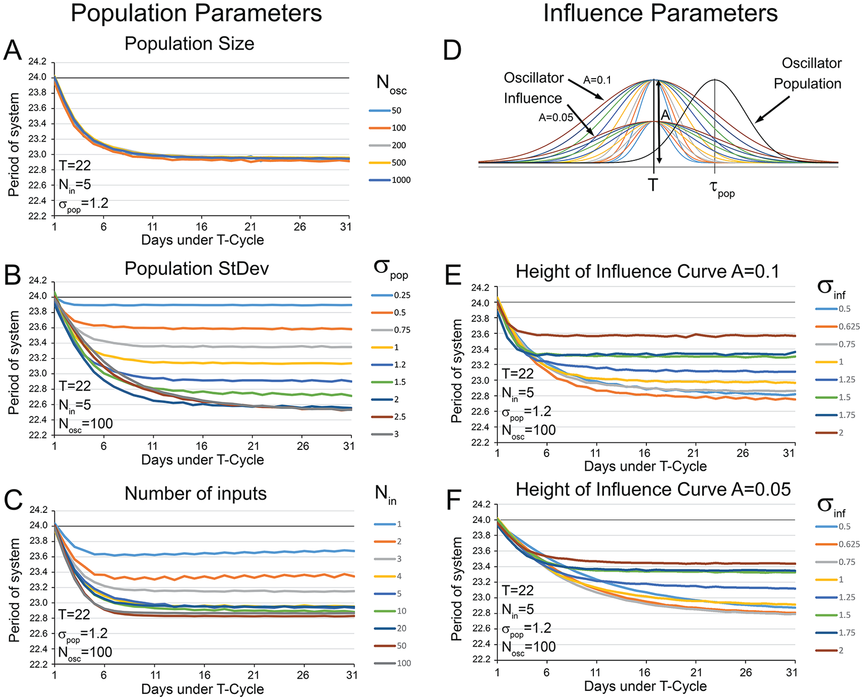
Simulations exploring population (A-C) parameters revealed that the number of oscillators used in each simulation (A) had very little influence on the after-effects observed. (B) Population standard deviation (σ_pop) had a strong influence on the magnitude of the after-effects observed. A small σ_pop (e.g., 0.25 h) produced a system that was quite resistant to T-cycle–induced after-effects. The largest and most rapidly induced after-effects were elicited with a σ_pop of 2 h. Simulations with larger σ_pop (e.g., 2.5-3 h) were able to reach the same final period but took longer to reach this asymptote. (C) The number of inputs (N_in) that each oscillator received had a minimal effect on the final after-effect period once a sufficient number of inputs was used (~4 inputs). Minor increases in the magnitude of the after-effects and the rate to achieve asymptote were observed with large N_in (e.g., 50-100) but represented at best minimal gains over much smaller numbers of inputs (e.g., 5). Simulations exploring parameters of the influence function (D-F) revealed that the magnitude of after-effects was affected by the width of this curve (σ_inf). Small width factors (σ_inf = 0.625 or 0.75) yielded the greatest magnitude after-effects. Smaller (σ_inf = 0.5) or larger (σ_inf ≥ 1.0) widths produced smaller magnitude after-effects. The height of the influence curve did not seem to influence the final magnitude of the after-effects. Taller influence curves (E, A = 0.1) reached their maximal magnitude after fewer iterations than did shorter influence curves (F, A = 0.05).

The variability of the populations from which these oscillators were drawn had an influence on how the system responded to T-cycles. Populations with lower variability were more resistant to the effects of the T-cycle and exhibited minimal after-effects (e.g., a period of about 23.9 h when σ_pop = 0.25). The overall influence of the T-cycle increased with variability. The most robust effect for T22 was observed with σ_pop = 2.0. Larger σ_pop values produced the same magnitude of effect as σ_pop = 2.0, but they required more iterations to reach the asymptote (Fig. 6B).

The number of inputs received by each oscillator had minimal influence once N_in > 4 (Fig. 6C). A single input produced weak after-effects. The amplitude of this effect increased further with 2, 3, or 4 connections. More inputs than this had minimal effect on the final period of the system, although the system reached its final period more quickly once each cell received 50 to 100 inputs.

Influence Parameters

Initially, the height of the influence curve was set to A = 0.1, with its width being specified by σ_inf = 1.0. Reducing the amplitude of the influence curve weakened the effect of the T-cycle on the system in that it required more iterations to reach asymptote. Given sufficient iterations of the simulation, final period of the system with A=0.05 was approximately the same as the final period when A=0.1. The width of the influence curve did have a prominent effect. The strongest effect of the 22-h T-cycle on the final period of the system was observed with σ_inf = 0.625 (Fig. 6D-F). As values of σ_inf increased or decreased from 0.625, the overall effect on the final period decreased.

Modeling In Vitro After-effects

Three studies have investigated after-effects in vitro following T-cycle exposure in vivo (Aton et al., 2004; Azzi et al., 2017; Molyneux et al., 2008), with the finding that short T-cycles produced long periods in vitro and vice versa. To explore what would be needed to replicate these observations with our model, we hypothesized that cells with greater influence would be more sensitive to cell death during the tissue slice preparation procedure, while those with lower influence would be more resistant because of their marginal role and connectivity in the system after prolonged T-cycle exposure. Initial simulations revealed that after prolonged T-cycle exposure, the overall variability of the periods of the oscillators in the system was quite low. As such, these simulations were run with a weaker system (A = 0.05, σ_inf = 0.6, N_in = 4). A threshold influence of 0.001 (output of equation 1) was selected (the maximal influence for any oscillator is 0.5 if its period matches T). Any cell with an influence greater than this value was eliminated, while any cell with an influence less than this value was retained (Fig. 7A). This threshold retained about 20% of the oscillators (18.7% of the oscillators for T22 and 19.4% of the oscillators for T26, based on 10 separate simulations each). The period of the system was determined before applying the threshold, to simulate the period of the system with all oscillators (the “before culture preparation” condition). The period was determined again after the threshold was applied, to simulate the period after selective loss of the influential cells (the “after culture preparation” condition). For T22, the periods of the system before application of the threshold ranged from 22.63 h to 23.37 h, while the periods ranged from 24.3 h to 24.89 h after the threshold was applied (Fig. 7B). For T26, the periods of the system before application of the threshold ranged from 24.79 h to 25.23 h, while the periods ranged from 22.86 h to 23.79 h after the threshold was applied (Fig. 7C). Of the original 100 oscillators in each simulation, between 11 and 32 oscillators survived in the T22 simulations, whereas between 12 and 27 survived in the T26 simulations.

Figure 7.

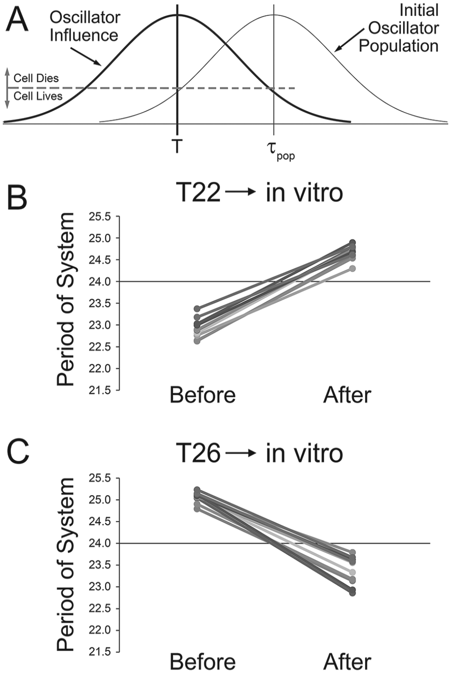
Simulations exploring whether selective cell death could explain the difference in after-effects observed between in vivo and in vitro observations. Animals exposed to short T-cycles will exhibit short periods in vivo but long periods in vitro. The opposite is observed for long T-cycles. A critical influence threshold was selected, and cells with an influence above this threshold were deemed to be strong participants in the neural network and, as such, were more sensitive to excitotoxic cell death. Cells with influences below this threshold were deemed to be too weak to be well integrated into the neural network and, as such, were relatively immune to excitotoxic cell death because of loss of inputs and outputs. The period of the ensemble was calculated with the strong cells included (before) and then excluded (after) to simulate their death during the slice-culture preparation procedure. Each simulation was run 10 times for both short (B) and long (C) T-cycles. The same pattern of periods was observed with these simulations, with short T-cycles leading to short periods in vivo but long periods in vitro and vice versa.

Discussion

The present model, in which cells that have a similar period to the imposed T-cycle have greater influence over the period of their targets and thus the overall circadian network, is able to reproduce the behavioral phenomenon of circadian after-effects following exposure to non–24-h T-cycles. Much as is observed with behavior, the period of the system following the end of the T-cycle is intermediate between the endogenous τ and the imposed T-cycle. A likely explanation for this observation can be extracted from Figure 2. Cells with periods similar to the T-cycle have the greatest individual influence, although they are not that numerous. The most numerous cells are those with periods close to the population mean, although they are not individually influential. Cells with periods intermediate to the population mean τ and the imposed T-cycle are both fairly numerous and fairly influential; thus, as a cluster, these cells will have the greatest aggregate influence on the system. Figure 2 also explains the limits observed in the range of T-cycles that yield prominent after-effects. T-cycles that differed from the population average τ by more than 3 h had diminishing effects, likely because of the scarcity of oscillators with periods this far from the population mean. The few oscillators with periods that would give them a strong influence in cases of these extreme T-cycles would have little effect on the system because of their overall low numbers.

The model makes interesting predictions about population parameters. While the SCN is composed of about 20,000 cells, many of which are cell-autonomous oscillators (Antle and Silver, 2005), our model performed identically with populations as small as 50 cells and as great as 1000 cells (Fig. 5A), suggesting that the number of cells has little influence on the phenomenon once the system is populated with a sufficient number of cells. In contrast, the variability of oscillator periods in the population had a prominent influence on the magnitude of after-effects. Populations with small standard deviations in period (e.g., 0.25 h; Fig. 6B) were quite robust and exhibited minimal after-effects, while those with large standard deviations (e.g., 2 h) had a maximal response. Interestingly, increasing the standard deviation further (e.g., 2.5-3 h) produced a system that could reach the same final τ but that required longer to reach this same steady state. The variability in periods for individual SCN neurons from wild-type animals has been reported to be as small as 0.8 h (mice; Herzog et al., 1998) and as large as 1.34 h (hamsters; Liu et al., 1997). Our simulation used an intermediate standard deviation, 1.2 h, based on the findings from rats (Welsh et al., 1995). Overall, as the standard deviation of the population periods increased, the magnitude of after-effects also increased. This would suggest that mutants that exhibited greater variability in periods between their individual SCN cells would exhibit greater magnitude after-effects. Mice that are heterozygous for the clock^Δ19 mutation and hamsters that carry either 1 or 2 copies of the tau mutation have greater variability in the distribution of their single-cell periods than is observed with wild-types (Herzog et al., 1998; Liu et al., 1997). Thus, the model would predict larger after-effects in these mutant animals than in their wild-type counterparts.

The final population parameter to consider is the number of synaptic connections. After-effects were still observed, with each cell receiving even just a single input (Fig. 6C). Four or 5 inputs per cell were sufficient to exhibit the full-magnitude response. This small number of connections is sufficient regardless of population size (Fig. 6A). When larger numbers of inputs were used (i.e., 50-100 inputs per cell), the system reached steady state a little more quickly and had only a modestly larger magnitude. Overall, 4 to 20 inputs per cell were sufficient to yield a realistic response. This small number of inputs falls within the range of axosomatic inputs received by individual SCN neurons, as estimated by ultrastructural analysis (i.e., 18-22 synapses; Güldner, 1984), only some of which would be intrinsic SCN-derived inputs, as many of these same cells also receive extra SCN inputs. In our simulations, when few connections are used, it is possible that through random connections, distinct noninteracting clusters are formed. This was not tracked, but given that such clusters would be randomly determined and assembled, and that the period of the system is derived independent of such clustering, these clusters, if and when they occur, would not influence the output of the model. Also, the spatial arrangements of the SCN are not considered here, but it is likely that the connections in the SCN are not random. It is likely that cells are connected to nearby cells that share similar rhythmic characteristics forming distinct functional clusters (Foley et al., 2011). It will be important to consider how the spatiotemporal organization of the SCN could influence plasticity, and these ideas are beginning to be explored (Azzi et al., 2017).

When animals are subjected to T-cycles, and their SCN subsequently examined in vitro using a luciferase reporter, the period of the SCN exhibits the opposite after-effect from what would be predicted based on behavior. Specifically, those exposed to short T-cycles in vivo have periods in vitro longer than 24 h and periods in vitro shorter than 24 h when exposed to long T-cycles (Aton et al., 2004; Molyneux et al., 2008). This was an unexpected finding, and various explanations have been forwarded, including a role for extra SCN oscillators (Aton et al., 2004; Molyneux et al., 2008) or methylation of genes in SCN cells in a region-specific manner (Azzi et al., 2017). To explore what would be needed to replicate these observations with our model, we tested the hypothesis that the inevitable cell death experienced during the slice preparation procedure may not be random but rather might select for the strongest cells in the network. This is analogous to what happens following a stroke, in which the ischemia leads to initial cell death. When glutamatergic cells die, they release large quantities of their neurotransmitters, resulting in secondary cell death in their targets (Szydlowska and Tymianski, 2010). Recent evidence suggests that this same excitotoxicity can occur in a glutamate-independent manner as well (Tehse and Taghibiglou, 2019), either through mechanical activation of NMDA receptors or other sources of enhanced calcium influx. As glutamate is the primary neurotransmitter of the retinohypothalamic tract (RHT), it is possible that retinorecipient SCN cells may also be highly sensitive to excitotoxicity during the SCN slice preparation. Plasticity events surrounding exposure to a T-cycle could change the strength and number of connections in the circadian network. Cells that are well integrated in the network would be more at risk since they receive and produce many strong connections. Cells with periods vastly different from the T-cycle may be protected due to plasticity events that lead to pruning of afferents and efferents for these outlier cells. Using this approach, we were able to replicate the observation that long T-cycles yield short periods when the strongest cells are removed from the network, thus mimicking selective cell death. Estimates of cell death following slice preparation, and determination of individual cell periods in a low-density culture following in vivo T-cycle exposure, could test the plausibility of such selective cell death contributing to the observation of in vivo/in vitro period difference mismatch. Nonetheless, these results do not exclude the possibility that the mismatch in period in vivo and in vitro may be due in part to loss of extra-SCN input, as has been suggested previously (Aton et al., 2004; Molyneux et al., 2008). Recently, extra-SCN oscillators have been shown to influence SCN period (Myung et al., 2018). In addition, nonphotic inputs related to activity can also influence circadian period (Edgar et al., 1991; Mrosovsky, 1999; Webb et al., 2014; Yamada et al., 1988), and loss of these inputs could also play a role in the change in period between the in vivo and in vitro situations.

Much of what is known about synaptic plasticity in the mammalian brain is based on experiments from long-term potentiation (LTP) in the hippocampus, where glutamate and the NMDA receptor play key roles. Glutamate is the primary neurotransmitter communicating light information from the RHT to SCN cells, and this pathway exhibits LTP following high-frequency stimulation of the optic nerve in an NMDA receptor–dependent manner (Fukunaga et al., 2002; Nishikawa et al., 1995; Nisikawa et al., 1998, 2002). While there is some evidence for glutamatergic transmission between SCN neurons (Michel et al., 2013), most (~70%) neurons in the SCN are GABAergic (Moore et al., 2002). Mechanisms of GABAergic plasticity are being elucidated and, like glutamate, are activity dependent (Flores and Mendez, 2014). Similar to plasticity at glutamatergic synapses, activity-dependent plasticity can be mediated by short-term biochemical changes (e.g., phosphorylation of receptors), modification of the ultrastructural character of the synapse (e.g., changes of the postsynaptic density and/or changes in the active zone of the axon terminal), or creation of new synapses (Flores and Mendez, 2014). There is evidence for remodeling of synapses (Gorostiza et al., 2014), dendrites, and axons (Frenkel and Ceriani, 2011) in the circadian system of flies. Furthermore, there is evidence that GABA, through the GABA_B receptor, mediates synaptic plasticity of retinal inputs to the SCN (Moldavan and Allen, 2013). Brain-derived neurotrophic factor, a major contributor to synaptogenesis (Cunha et al., 2010), is found in the SCN and contributes to circadian responses to light (Allen and Earnest, 2005; Allen et al., 2005; Liang et al., 2000; Liang et al., 1998). LHX1, a gene that plays a role in the circadian system in axon terminal differentiation and SCN development (VanDunk et al., 2011), also participates in plasticity of the SCN in adulthood, particularly with respect to phase coupling and synchrony between oscillators (Bedont et al., 2014; Hatori et al., 2014). These mechanisms could underlie synaptic plasticity in the circadian network. Such plasticity is supported by recent observations in the reorganization of the SCN network following exposure to T-cycles. Specifically, exposure to T-cycles reorganizes the phase relationship between different SCN regions, with short T-cycles leading to a phase-delayed dorsal SCN and long T-cycles leading to a phase-delayed ventral SCN (Azzi et al., 2017). These changes are dependent on synaptic communication, as blocking action potentials reversed these period changes, demonstrating their activity dependence (Azzi et al., 2017).

Plasticity can also be mediated through epigenetic mechanisms. After-effects due to T-cycle exposure lead to altered methylation of a wide variety of genes (Azzi et al., 2014). When changes to DNA methylation are blocked with zebularine, a DNA methyltransferase inhibitor, the magnitude of after-effects is significantly diminished (Azzi et al., 2014). These methylation changes appear to be region specific (Azzi et al., 2017). Such epigenetic changes are consistent with our current model. While the present model highlights a role for activity-dependent synaptic plasticity, our model does require changes in the period of individual clock cells. While our model suggests that the new period of a cell is a function of its own period and the influence-weighted periods of its afferent cells, the mechanism by which such a period change is mediated within this target cell is unspecified in our model but could be dependent on epigenetic changes. The genes that experience such epigenetic changes still need to be determined. It is likely that many of the core clock genes are not individually necessary for after-effects, as after-effects are still observed in animals lacking one of Per1, Per2, Per3, and Clock (Beaule and Cheng, 2011; Pendergast et al., 2010). This is consistent with the methylation screen following T-cycle–induced after-effects, in which genes for neurotransmitter receptors and ion channels represented the genes with the greatest changes in methylation (Azzi et al., 2017).

A number of other mathematical models have been suggested to explain after-effects. Two of these explore the role of the phase of the individual oscillators within the population (Beersma et al., 2017; Bordyugov and Herzel, 2014). Beersma and colleagues (2017) explored the role of phase dispersion on the period of the overall output of the circadian oscillator. They demonstrated that the period of the ensemble lengthens as phase coherence increases and that as synchrony is reduced, the period of the ensemble shortens. They suggest that plastic changes in the period of the ensemble could be mediated by alterations in phase dispersion of units in the network. Bordyugov and Herzel (2014) explored the role that phase coherence could have on coupling strength between SCN oscillator cells. When cells had similar phases, their coupling strength was high, resulting in LTP of their coupling. When cells had opposite phases, their coupling strength was negative, resulting in long-term depression of their coupling. This led to coupling between oscillators with periods close to the population mean, and this subsequent phase coherence led to their dominance over the whole network. When a T-cycle is applied, greater phase coherence is achieved for oscillators with periods closer to the applied T-cycle, thereby driving the ensemble period toward that of the applied T-cycle. A third model to explore plasticity of the SCN period also used a phase approach, treating the SCN as being composed of 2 oscillators, representing the dorsal and ventral parts of the SCN (Azzi et al., 2017). Phase relationships between these regions can explain after-effects, particularly those observed in vitro following in vivo T-cycle exposure. The present model explores only the period of the oscillators and does not consider how phase could strengthen interactions between oscillators. The SCN exhibits regional clustering of oscillator cells in terms of phase and period (Foley et al., 2011). While connections between oscillators in our model are random with respect to period, it is likely that cells would be more closely connected to their neighbors, which would share similar phases and periods. Such an arrangement should strengthen the changes observed within our model. Thus, while these other models differ in their approach to exploring SCN plasticity, their approaches are compatible with those that we explore here, and each of these different approaches should only reinforce each other if they are combined.

Our model explored only the period of each cell, independent of other parameters such as phase, amplitude, and location. In reality, the SCN is composed of a variety of oscillators with specific spatiotemporal organization (Evans et al., 2011; Hamada et al., 2004), some of which are more robust than others (Webb et al., 2009). Many of these features are also likely to influence how clock cells interact and influence each other’s periods.

The present model is able to replicate the phenomenon of T-cycle–induced after-effects by modifying synaptic strength as a function of how similar a cell’s period is to the imposed T-cycle. The altered synaptic strength then influences the degree to which this cell can influence the periods of its target cells. The mechanism by which this plasticity is mediated at the synaptic level is unspecified here but most closely matches more subtle plastic changes in which the strength of the connection is altered without altering the number of connections. Future iterations of this model could explore the contribution of additional physical changes, such as adding de novo synaptic connections for strong cells with periods close to that of the imposed T-cycle and pruning inputs and outputs from weaker cells with periods different from the imposed T-cycle. Overall, this model highlights a role for synaptic plasticity in the circadian network.

Footnotes

Conflict Of Interest Statement

The authors have no potential conflicts of interest with respect to the research, authorship, and/or publication of this article.

ORCID iD

Michael C. Antle

References

Agnihotri

Lopez-Garcia

Hawkins

Arancio

(1998) Morphological changes associated with long-term potentiation. Histol Histopathol 13:1155-1162.

Allen

Earnest

(2005) Overlap in the distribution of TrkB immunoreactivity and retinohypothalamic tract innervation of the rat suprachiasmatic nucleus. Neurosci Lett 376:200-204.

Allen

Earnest

(2005) TrkB-deficient mice show diminished phase shifts of the circadian activity rhythm in response to light. Neurosci Lett 378:150-155.

Antle

Foley

Silver

(2003) Gates and oscillators: a network model of the brain clock. J Biol Rhythms 18:339-350.

Antle

Foley

Silver

(2007) Gates and oscillators II: zeitgebers and the network model of the brain clock. J Biol Rhythms 22:14-25.

Antle

Silver

(2005) Orchestrating time: arrangements of the brain circadian clock. Trends Neurosci 28:145-151.

Aton

Block

Tei

Yamazaki

Herzog

(2004) Plasticity of circadian behavior and the suprachiasmatic nucleus following exposure to non-24-hour light cycles. J Biol Rhythms 19:198-207.

Azzi

Dallmann

Casserly

Rehrauer

Patrignani

Maier

Kramer

Brown

(2014) Circadian behavior is light-reprogrammed by plastic DNA methylation. Nat Neurosci 17:377-382.

Azzi

Evans

Leise

Myung

Takumi

Davidson

Brown

(2017) Network dynamics mediate circadian clock plasticity. Neuron 93:441-450.

10.

Bailey

Giustetto

Huang

Hawkins

Kandel

(2000) Is heterosynaptic modulation essential for stabilizing Hebbian plasticity and memory? Nat Rev Neurosci 1:11-20.

11.

Beaule

Cheng

(2011) The acetyltransferase Clock is dispensable for circadian aftereffects in mice. J Biol Rhythms 26:561-564.

12.

Bedont

LeGates

Slat

Byerly

Wang

Rupp

Qian

Wong

Herzog

et al. (2014) Lhx1 controls terminal differentiation and circadian function of the suprachiasmatic nucleus. Cell Rep 7:609-622.

13.

Beersma

DGM

Gargar

Daan

(2017) Plasticity in the period of the circadian pacemaker induced by phase dispersion of its constituent cellular clocks. J Biol Rhythms 32:237-245.

14.

Bernardinelli

Nikonenko

Muller

(2014) Structural plasticity: mechanisms and contribution to developmental psychiatric disorders. Front Neuroanat 8:123.

15.

Bordyugov

Herzel

(2014) The suprachiasmatic nucleus as a network of coupled oscillators: adaptation by learning. In: Honma

, editor. Dynamics of circadian oscillation in the SCN. Hokkaido (Japan): Hokkaido University Press. p. 173-184.

16.

Boulos

Macchi

Terman

(2002) Twilights widen the range of photic entrainment in hamsters. J Biol Rhythms 17:353-363.

17.

Cunha

Brambilla

Thomas

(2010) A simple role for BDNF in learning and memory? Front Mol Neurosci 3:1.

18.

Edgar

Martin

Dement

(1991) Activity feedback to the mammalian circadian pacemaker: influence on observed measures of rhythm period length. J Biol Rhythms 6:185-199.

19.

Evans

Leise

Castanon-Cervantes

Davidson

(2011) Intrinsic regulation of spatiotemporal organization within the suprachiasmatic nucleus. PLoS One 6:e15869.

20.

Flores

Mendez

(2014) Shaping inhibition: activity dependent structural plasticity of GABAergic synapses. Front Cell Neurosci 8:327.

21.

Foley

Tong

Foley

Lesauter

Welsh

Silver

(2011) Characterization of orderly spatiotemporal patterns of clock gene activation in mammalian suprachiasmatic nucleus. Eur J Neurosci 33:1851-1865.

22.

Forrest

Parnell

Penzes

(2018) Dendritic structural plasticity and neuropsychiatric disease. Nat Rev Neurosci 19:215-234.

23.

Frenkel

Ceriani

(2011) Circadian plasticity: from structure to behavior. Int Rev Neurobiol 99:107-138.

24.

Fukunaga

Horikawa

Shibata

Takeuchi

Miyamoto

(2002) Ca2+/calmodulin-dependent protein kinase II-dependent long-term potentiation in the rat suprachiasmatic nucleus and its inhibition by melatonin. J Neurosci Res 70:799-807.

25.

Gorostiza

Depetris-Chauvin

Frenkel

Pirez

Ceriani

(2014) Circadian pacemaker neurons change synaptic contacts across the day. Curr Biol 24:2161-2167.

26.

Güldner

(1984) Suprachiasmatic nucleus: numbers of synaptic appositions and various types of synapses: a morphometric study on male and female rats. Cell Tissue Res 235:449-452.

27.

Hamada

Antle

Silver

(2004) Temporal and spatial expression patterns of canonical clock genes and clock-controlled genes in the suprachiasmatic nucleus. Eur J Neurosci 19:1741-1748.

28.

Hatori

Gill

Mure

Goulding

O’Leary

Panda

(2014) Lhx1 maintains synchrony among circadian oscillator neurons of the SCN. Elife 3:e03357.

29.

Hebb

(1949) Organization of behavior. New York: John Wiley & Sons.

30.

Herzog

Takahashi

Block

(1998) Clock controls circadian period in isolated suprachiasmatic nucleus neurons. Nat Neurosci 1:708-713.

31.

Liang

Allen

Earnest

(2000) Role of brain-derived neurotrophic factor in the circadian regulation of the suprachiasmatic pacemaker by light. J Neurosci 20:2978-2987.

32.

Liang

Sohrabji

Miranda

Earnest

(1998) Expression of brain-derived neurotrophic factor and its cognate receptor, TrkB, in the rat suprachiasmatic nucleus. Exp Neurol 151:184-193.

33.

Liu

Weaver

Strogatz

Reppert

(1997) Cellular construction of a circadian clock: period determination in the suprachiasmatic nuclei. Cell 91:855-860.

34.

Meijer

Michel

Vanderleest

Rohling

(2010) Daily and seasonal adaptation of the circadian clock requires plasticity of the SCN neuronal network. Eur J Neurosci 32:2143-2151.

35.

Michel

Marek

Vanderleest

Vansteensel

Schwartz

Colwell

Meijer

(2013) Mechanism of bilateral communication in the suprachiasmatic nucleus. Eur J Neurosci 37:964-971.

36.

Moldavan

Allen

(2013) GABAB receptor-mediated frequency-dependent and circadian changes in synaptic plasticity modulate retinal input to the suprachiasmatic nucleus. J Physiol 591:2475-2490.

37.

Molyneux

Dahlgren

Harrington

(2008) Circadian entrainment aftereffects in suprachiasmatic nuclei and peripheral tissues in vitro. Brain Res 1228:127-134.

38.

Moore

Speh

Leak

(2002) Suprachiasmatic nucleus organization. Cell Tissue Res 309:89-98.

39.

Mrosovsky

(1999) Further experiments on the relationship between the period of circadian rhythms and locomotor activity levels in hamsters. Physiol Behav 66:797-801.

40.

Myung

Schmal

Hong

Tsukizawa

Rose

Zhang

Holtzman

De Schutter

Herzel

Bordyugov

et al. (2018) The choroid plexus is an important circadian clock component. Nat Commun 9:1062.

41.

Nishikawa

Shibata

Watanabe

(1995) Circadian changes in long-term potentiation of rat suprachiasmatic field potentials elicited by optic nerve stimulation in vitro. Brain Res 695:158-162.

42.

Nisikawa

Shimazoe

Shibata

Watanabe

(1998) N-methyl-D-aspartate receptors are indispensable for the formation of long-term potentiation in the rat suprachiasmatic nucleus in vitro. Brain Res 782:303-305.

43.

Nisikawa

Shimazoe

Shibata

Watanabe

(2002) Time-dependent effect of glutamate on long-term potentiation in the suprachiasmatic nucleus of rats. Jpn J Pharmacol 90:201-204.

44.

Pendergast

Friday

Yamazaki

(2010) Photic entrainment of period mutant mice is predicted from their phase response curves. J Neurosci 30:12179-12184.

45.

Pittendrigh

(1960) Circadian rhythms and the circadian organization of living systems. Cold Spring Harbor Symp Quant Biol 25:159-184.

46.

Pittendrigh

(1964) The entrainment of circadian oscillations by light and their role as photoperiodic clocks. Am Nat 98:261-294.

47.

Pittendrigh

Daan

(1976) A functional analysis of circadian pacemakers in nocturnal rodents. I. The stability and lability of spontaneous frequency. J Comp Physiol 106:223-252.

48.

Rohling

Meijer

VanderLeest

Admiraal

(2006) Phase differences between SCN neurons and their role in photoperiodic encoding; a simulation of ensemble patterns using recorded single unit electrical activity patterns. J Physiol Paris 100:261-270.

49.

Schaap

Albus

VanderLeest

Eilers

Detari

Meijer

(2003) Heterogeneity of rhythmic suprachiasmatic nucleus neurons: Implications for circadian waveform and photoperiodic encoding. Proc Natl Acad Sci U S A 100:15994-15999.

50.

Szydlowska

Tymianski

(2010) Calcium, ischemia and excitotoxicity. Cell Calcium 47:122-129.

51.

Tehse

Taghibiglou

(2019) The overlooked aspect of excitotoxicity: glutamate-independent excitotoxicity in traumatic brain injuries. Eur J Neurosci 49:1157-1170.

52.

VanderLeest

Houben

Michel

Deboer

Albus

Vansteensel

Block

Meijer

(2007) Seasonal encoding by the circadian pacemaker of the SCN. Curr Biol 17:468-473.

53.

VanDunk

Hunter

Gray

(2011) Development, maturation, and necessity of transcription factors in the mouse suprachiasmatic nucleus. J Neurosci 31:6457-6467.

54.

Webb

Angelo

Huettner

Herzog

(2009) Intrinsic, nondeterministic circadian rhythm generation in identified mammalian neurons. Proc Natl Acad Sci U S A 106:16493-16498.

55.

Webb

Antle

Mistlberger

(2014) Regulation of circadian rhythms in mammals by behavioral arousal. Behav Neurosci 128:304-325.

56.

Weisgerber

Redlin

Mrosovsky

(1997) Lengthening of circadian period in hamsters by novelty-induced wheel running. Physiol Behav 62:759-765.

57.

Welsh

Logothetis

Meister

Reppert

(1995) Individual neurons dissociated from rat suprachiasmatic nucleus express independently phased circadian firing rhythms. Neuron 14:697-706.

58.

Yamada

Shimoda

Ohi

Takahashi

(1988) Free-access to a running wheel shortens the period of free-running rhythm in blinded rats. Physiol Behav 42:87-91.

Modeling the Influence of Synaptic Plasticity on After-effects

Abstract

Keywords

Materials And Methods

Model

Standard Simulations

T-cycle to DD Simulations

In Vivo to In Vitro Simulations

Results

Initial Simulations

Exploring Variability

T-cycle to DD Simulations

Oscillator Population Parameters

Influence Parameters

Modeling In Vitro After-effects

Discussion

Footnotes

Conflict Of Interest Statement

ORCID iD

References