Novel Light/Dark Regimens with Minimum Light Promote Circadian Disruption: Simulations with a Model Oscillator

Abstract

Artificial lab manipulation of LD cycles has enabled simulations of the disruptive conditions found in modern human societies, such as jet-lag, night-work and light at night. New techniques using animal models have been developed, and these can greatly improve our understanding of circadian disruption. Some of these techniques, such as in vivo bioluminescence assays, require minimum external light. This requirement is challenging because the usual lighting protocols applied in circadian desynchronization experiments rely on considerable light input. Here, we present a novel LD regimen that can disrupt circadian rhythms with little light per day, based on computer simulations of a model limit-cycle oscillator. The model predicts that a single light pulse per day has the potential to disturb rhythmicity when pulse times are randomly distributed within an interval. Counterintuitively, the rhythm still preserves an underlying 24-h periodicity when this interval is as large as 14 h, indicating that day/night cues are still detectable. Only when pulses are spread throughout the whole 24-h day does the rhythm lose any day-to-day period correlation. In addition, the model also reveals that stronger pulses of brighter light should exacerbate the disrupting effects. We propose the use of this LD schedule—which would be compatible with the requirements of in vivo bioluminescence assays—to help understand circadian disruption and associated illnesses.

In mammals, circadian rhythms in physiology and behavior are driven by a pacemaker located in the SCN of the hypothalamus, which coordinates the timing of peripheral oscillators in many body tissues (Dibner et al., 2010; Welsh et al., 2010). Whereas locomotor activity rhythms provide indirect measurements of the period and phase of the SCN, several techniques have enabled more direct assessment of these pacemaker properties. Bioluminescence reporters provided the first direct measurements of period and phase of clock-gene expression from cultured SCN and peripheral tissues in vitro (Yamazaki et al., 2000). In this approach, explant tissues are monitored in constant darkness, and all oscillator properties are assessed as after-effects (Pittendrigh and Daan, 1976) of conditions experienced by the organism before tissue collection. Recent technical advances have allowed real-time monitoring of clock-gene expression over several days in immobilized intact animals (Tahara et al., 2012) and, more recently, even in freely moving laboratory rodents (Hamada et al., 2016; Ono et al., 2015; Saini et al., 2013; Yamaguchi et al., 2016). With these new approaches, clock properties can be assessed continuously in the whole organism, preserving in vivo systemic interactions within the body.

Human shift-work, night-work and jet-lag promote desynchrony of the circadian system to the day/night environment and have been associated with an increased risk of different illnesses (Golombek et al., 2013; Kalsbeek et al., 2011; Karatsoreos et al., 2011; Scheer et al., 2009). Various experimental protocols have been applied to model circadian disruption with artificial LD manipulation in laboratory rodents (Fisk et al., 2018), such as constant light (Ohta et al., 2005), simulated jet-lag (Albus et al., 2005; Davidson et al., 2009; Nagano et al., 2003; Yamaguchi et al., 2013; Yamazaki et al., 2000), chronic jet-lag (Casiraghi et al., 2012; Davidson et al., 2006), and forced desynchronization (Cambras et al., 2007; de la Iglesia et al., 2004; Schwartz et al., 2009). In vivo reporter bioluminescence assays offer a unique opportunity to study the effects of circadian disruption on oscillator properties, enabling real-time monitoring of clock gene expression in intact, freely moving animals exposed to disrupting light regimes. However, since clock information is also itself obtained through the detection of light emitted by tissues, experimental light cycles in these assays should carry as little external light as possible.

We propose a novel LD regimen with minimum light input that can potentially induce circadian disruption. This extreme LD paradigm has been inspired by previous modeling studies that sought something else, namely, the minimum light timing to achieve entrainment in subterranean rodents. Computer simulations predicted that, for entrainment, it suffices to apply one single light pulse per day occurring at a random time within a pre-defined daytime interval (Flôres et al., 2013), and this was confirmed experimentally (Flôres et al., 2016). Surprisingly, the daytime interval, that here we name “I”, could be as wide as 14 h. Of note, this entrainment protocol has less timing constraints than the classic 24-h T-cycle that consists of a single pulse applied at the same time each day. Upon increasing the “I” interval even further, with gradual scattering of daily single pulses throughout the 24 h, there was eventually a complete loss of day/night cues. Consequently, entrainment was finally lost (Flôres et al., 2013), and this was confirmed by an increase in side-band peaks in periodograms.

Here, we present further computer simulations predicting that this extreme lighting regimen, with “I” values of 24 h, can potentially disrupt the rhythmicity of circadian oscillators. We propose that this protocol fulfills the requirements for minimal light input to be used with in vivo bioluminescence assays in studies of circadian disruption.

In our simulations, we used a limit-cycle Pavlidis-Pittendrigh oscillator, as described in previous rodent models (Oda et al., 2000). Pittendrigh’s standard set of parameters was used, which had been developed for Drosophila eclosion simulations (Pittendrigh et al., 1991). By means of computer simulations in the NeuroDynamix software (Friesen and Friesen, 1994), the model oscillator was subjected to daily 1-h pulses, applied only once per day, at random times uniformly distributed within the “I” interval (Flôres et al., 2013). The size of the interval was set to either 4, 14, or 24 h (I = 4 h, 14 h or 24 h). Pulse times were obtained with the RANDBETWEEN function in Microsoft Excel (2007), which uses the Wichmann-Hill algorithm for random number generation (Wichmann and Hill, 1982). Phase-response curves to the 1-h pulse were generated by applying individual pulses every 2 circadian hours in constant conditions. Steady-state phase shifts were calculated as the difference between the peak time of the oscillator variable and the peak time of a reference (unpulsed) oscillator.

We first applied schedules with pulses of low amplitude, representing a low light intensity, here referred to as “weak pulses.” In response to weak pulses at random times, the activity rhythm of the oscillator was synchronized to a 24-h period (Fig. 1A, B) for distribution intervals of 4 h and 14 h. When the interval was further increased to I = 24 h, entrainment was lost but the integrity of the rhythm was maintained (Fig. 1C). We refer to these pulses as “weak,” because they generate a type-1 phase-resetting (Winfree, 1980), as illustrated by the phase-response curve to the stimulus (Fig. 1G).

Figure 1.

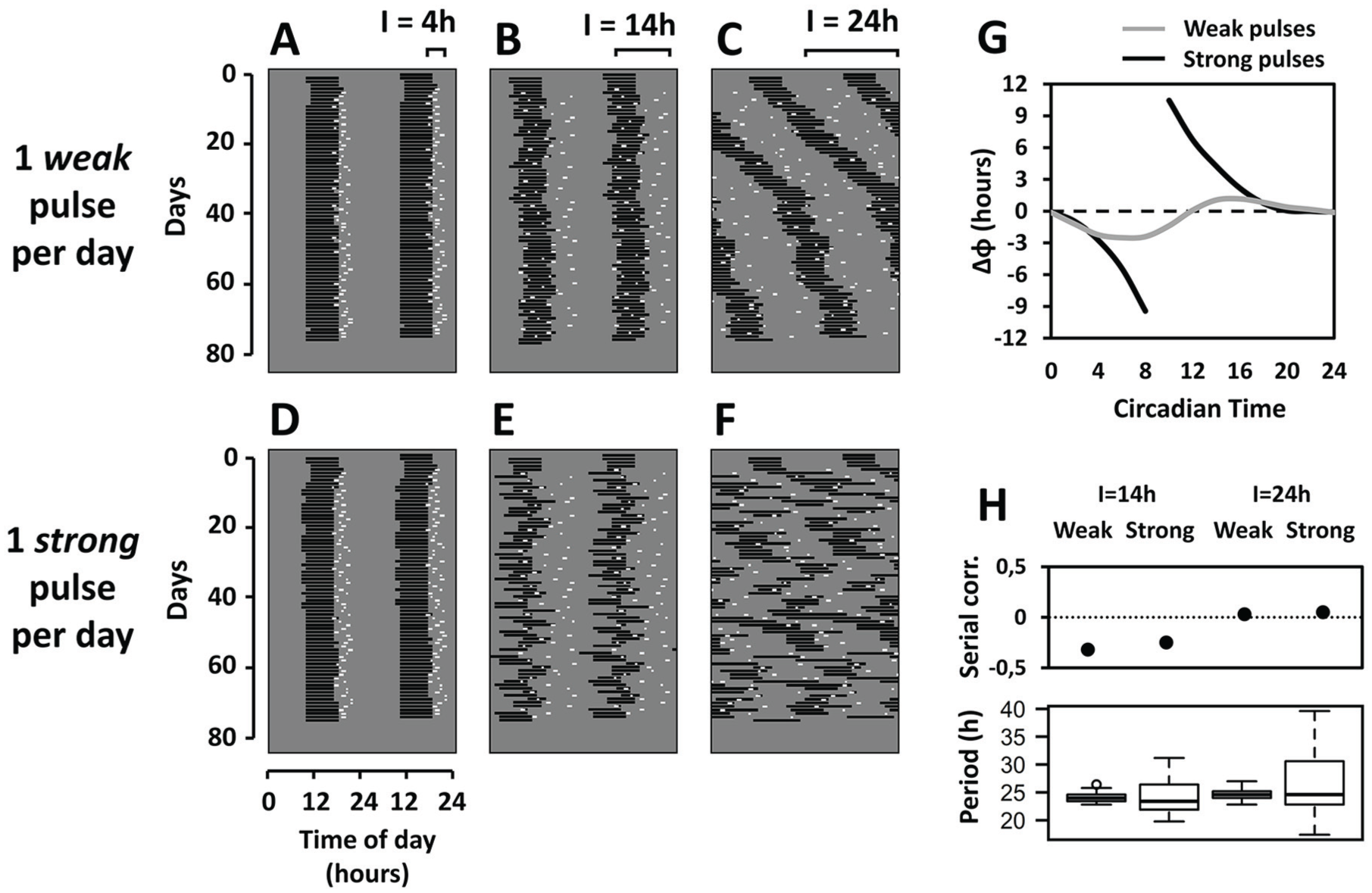
Rhythms of the model oscillator exposed to randomly timed light pulses for 70 days. Pulses starting on day 5 were applied only once per day at a random time within a daily interval “I”. (A-F) Double-plotted actograms illustrate the daily activity phase of the oscillator (horizontal black lines) and the simulated light pulses (white dots) in otherwise constant darkness (gray background). The same pulse schedules were used for weak pulses (A-C) and strong pulses (D-F). Axes are depicted in the lower-left graph. Brackets above the upper graphs indicate the “I” interval within which pulse times are uniformly distributed. I = 4 h and I = 24 h “weak pulse” simulations are modified from Flôres et al. (2013). (G) Phase-response curves to the weak and strong pulses. (H) Analysis of the day-to-day period values of the oscillator exposed to weak and strong pulses at I = 14 h and I = 24 h. Upper: serial correlation (Pearson’s r coefficient) between consecutive periods (zero dotted line means no correlation). Lower: boxplot representation of the period distributions. Oscillator parameter values: a = 0.85, b = 0.3, c = 0.8, d = 0.5. Pulse duration: 1 h. Pulse amplitude: 1.1 arbitrary units (weak pulses) or 10.0 arbitrary units (strong pulses).

With the same schedules, we next tested the effects of pulses with high amplitude, which simulate brighter light. These “strong pulses” also entrained the oscillator rhythm to 24 h when pulse times were randomly distributed within intervals of 4 h and 14 h (Fig. 1D, E). However, the phase of the oscillator was noticeably more variable throughout the days. With a wider interval of I = 24 h, the rhythm was not only desynchronized but its coherence among consecutive days was also lost, displaying complete disruption (Fig. 1F). We define these pulses as “strong” based on their type-0 phase-resetting properties (Winfree, 1980), as evidenced by the associated phase-response curve (Fig. 1G).

To quantify the disruption in rhythmic patterns, we initially measured the variability of day-to-day periods in the I = 14 h and I = 24 h schedules with both weak and strong pulses. The middle of activity on each day was chosen as a reference phase and the day-to-day period was measured as the interval between the reference phases on each day and the following day. Period values within each regimen were not normally distributed (Shapiro-Wilk normality test, P < 0.005 in the 4 regimens). Therefore, we applied a Brown-Forsythe test to verify unequal variances in the periods among pulse schedules, which confirmed statistical differences (F = 9.14, df1 = 3, df2=108.16, P < 0.00005) (Fig. 1H, lower). A post-hoc pairwise Tukey test on the residuals from period medians indicated significant differences in period variability among all pulse regimens (P < 0.005) except between the two I = 14 h regimens (P = 0.98). These results suggest that stronger pulses impose greater period variation. However, visual inspection of the actograms indicates that the I = 14 h regimen under strong pulses still preserves a 24-h component, which cannot be detected under I = 24 h regimens (Fig. 1C, F). Therefore, we next quantified the serial correlation between consecutive periods (adapted from Pittendrigh and Daan, 1976 apud Forger, 2017) as a second measurement of disruption. Both I = 14 h regimens presented negative values for the correlation coefficient (weak: r = −0.32, strong: r = −0.25), which indicates that, despite period variations, there is still an underlying periodicity (Fig. 1H, upper). In contrast, both I = 24 h schedules returned near zero values for the correlation (weak: r = 0.03, strong: r = 0.05), implying greater overall disruption (Fig. 1H, upper). Analyses were performed in R version 3.5.0.

We have explored a limited set of other pulse amplitudes and “I”-interval combinations with the same oscillator configuration and pulse duration. These simulations confirmed that pulse schedules are disruptive only for pulse amplitudes above 4 (arbitrary units), which is the lower limit for type-0 resetting. Within this amplitude range, disruption is restricted to “I” intervals of 16 h or more. Specific (amplitude × interval) thresholds for disruption should be quantitatively different depending on oscillator configuration and pulse duration. However, we predict that the qualitative pattern relative to type-1/type-0 resetting should remain regardless of parameter choice. Simulations with the model oscillator have revealed a novel LD regimen that can potentially be used to induce circadian rhythm disruption. The unique light schedule fulfills the requirements of little light per day and could thus be applied concomitantly with in vivo recordings of bioluminescence reporter-genes, to impose rhythm disruption in freely moving laboratory animals. Furthermore, since our generic oscillator model has no a priori compromise to specific biochemical mechanisms, we predict that results can be extrapolated to any organism and level of biological organization. Rhythms from whole plants, arthropods, vertebrates, or even tissue explants can be potentially disrupted with strong and randomly timed pulses.

In our simulations, we used pulses of 1-h duration. For in vivo monitoring of bioluminescent reporters, it may be advantageous to use shorter pulses. A strong pulse is defined here as one that promotes large phase-shifts associated with a type-0 phase-response curve. The response to light in the circadian system of mammals expresses a reciprocity between duration and irradiance of the light stimulus. It is the total photon count, rather than the duration or irradiance alone, that dictates responses to light. This has been confirmed at different levels of organization, such as in behavioral phase-shifts (Nelson and Takahashi, 1991, 1999) and in the expression of Fos (Dkhissi-Benyahya et al., 2000) or clock genes (Shigeyoshi et al., 1997) in the SCN. Therefore, shorter pulses with brighter light should be equally effective in inducing strong phase-resetting and, thus, in promoting the desynchronizing effects predicted in our model.

Other protocols, such as forced desynchronization, simulated jet-lag, and chronic jet-lag, have usually applied full LD cycles; however, the disrupting effects can be well reproduced using single-pulse T-cycles instead (Casiraghi et al., 2012). In this sense, non-24-h single-pulse T-cycles also fulfill the minimum light input requirement of in vivo bioluminescence assays. Interestingly, although we aimed for a protocol of minimal light, Fukuda et al. (2013) presented a complementary approach of dark pulses in a light background, disrupting rhythmicity in Arabidopsis. They used yet another protocol to induce disruption, by taking the oscillator to its singularity (Winfree, 1980, Engelmann et al., 1978, Huang et al., 2006). This could also be interesting for in vivo studies requiring only one light pulse. However, the resulting arrhythmicity is unstable and would not provide sustained disruption.

Our I = 24 h random-pulse protocol with strong light pulses breaks apart the output activity rhythm, sparing no day-to-day period correlation (Fig. 1H). This pattern results from an oscillator that is bombarded daily by strong pulses at random phases, shifting the oscillator to random directions (Fig. 1F). Interestingly, however, these same strong and randomly timed pulses do entrain the same oscillator if the “I” interval offers a reminiscent day/night cue (Fig. 1E). Individual variability is expected in the response to light pulses due to variations in light perception, oscillator period, and phase-resetting properties. This can result in each individual experiencing a disruption of different magnitude when exposed to the same pulse schedule. Higher pulse strengths should, however, guarantee a greater proportion of fully disrupted individuals. For instance, we previously applied randomly timed pulses in subterranean rodents (Flôres et al., 2016) and observed that, when pulse times were distributed in a wide interval of 20 h, a single animal already presented disruption of the activity rhythm. The light intensity in that study promoted weak (type-1) phase resetting (Flôres et al., 2013); however, it is possible that the referred individual was more sensitive to light and perceived strong pulses, which would agree with our current model.

We hope this new light schedule can be useful for future investigations on circadian disruption and that it fosters new discoveries on the importance of a coherent internal timing to human and animal health.