Entrainment Maps

Abstract

Circadian oscillators found across a variety of species are subject to periodic external light-dark forcing. Entrainment to light-dark cycles enables the circadian system to align biological functions with appropriate times of day or night. Phase response curves (PRCs) have been used for decades to gain valuable insights into entrainment; however, PRCs may not accurately describe entrainment to photoperiods with substantial amounts of both light and dark due to their reliance on a single limit cycle attractor. We have developed a new tool, called an entrainment map, that overcomes this limitation of PRCs and can assess whether, and at what phase, a circadian oscillator entrains to external forcing with any photoperiod. This is a 1-dimensional map that we construct for 3 different mathematical models of circadian clocks. Using the map, we are able to determine conditions for existence and stability of phase-locked solutions. In addition, we consider the dependence on various parameters such as the photoperiod and intensity of the external light as well as the mismatch in intrinsic oscillator frequency with the light-dark cycle. We show that the entrainment map yields more accurate predictions for phase locking than methods based on the PRC. The map is also ideally suited to calculate the amount of time required to achieve entrainment as a function of initial conditions and the bifurcations of stable and unstable periodic solutions that lead to loss of entrainment.

The ability of circadian oscillators to entrain to daily cycles of light and temperature has been called both the most important and the most misunderstood property of circadian rhythmicity (Johnson et al., 2003). Entrainment implies that an endogenous oscillator has matched its period to that of an external periodic forcing and has established a stable phase relationship with the forcing signal. The process of circadian entrainment has been studied extensively using tools from dynamical systems and oscillator theory (Ananthasubramaniam et al., 2014; Bagheri et al., 2008; Bordyugov et al., 2013a; Gu et al., 2012, 2013; Indic et al., 2006; Johnson et al., 2003; Leise and Siegelmann, 2006; Leloup and Goldbeter, 2013; Ramkisoensing et al., 2014; Rand et al., 2004; Roenneberg et al., 2003; Serkh and Forger, 2014; Woller et al., 2014). Perhaps the most commonly used method relies on phase response curves (PRCs) that measure the change in the phase of an endogenous limit cycle oscillation (typically in constant darkness or DD) induced by a perturbation (typically a light pulse) as a function of the phase at which the perturbation is applied (Johnson, 1999). Alternatively, one could perturb an oscillator in constant light (LL) with dark pulses. Such PRCs can be constructed for light or dark pulses of arbitrary strength and duration. However, for a PRC to accurately predict properties of entrainment to periodic light or dark pulses, the perturbations must be weak or brief enough that the oscillator relaxes back to the DD or LL limit cycle attractor before the next pulse arrives. Since circadian oscillators are naturally subject to forcing in which the light duration is several hours followed by several hours of darkness, the PRC may not be ideally suited to accurately determine entrainment in this context. In fact, we show that PRCs do not accurately predict the phase of entrainment in 3 different mathematical models of circadian clocks that are subjected to photoperiods with substantial amounts of both light and dark, such as 12-h:12-h light-dark (12:12 LD) cycles. For these LD cycles, the entrained solution is best thought of as a combination of 2 limit cycle attractors (i.e., the DD and LL limit cycles), rather than as a perturbation of a single limit cycle attractor (Peterson, 1980).

In this paper, we introduce a new tool, a 1-dimensional entrainment map, which is not based on perturbing the DD or LL oscillator. Instead, the map uses information on how both the 12-h light period and the 12-h dark period affect cycle duration as a function of the time elapsed since the lights last turned on. We show that the stable fixed point of the map corresponds to a stable LD-entrained solution. Properties of the entrained solution, such as the range of entrainment as a function of parameters or the speed with which entrainment occurs, are then inferred from properties of the map. We demonstrate that the map accurately predicts the phase of entrainment independent of the photoperiod across a variety of different models. Our findings are consistent with previous results in the literature (Bordyugov et al., 2015; Granada et al., 2013) and provide a new method for studying high-dimensional circadian models that are difficult to analyze mathematically.

The entrainment map is an example of an iterated map, a class of dynamical systems in which time is treated as discrete rather than continuous (Strogatz, 1994; Wu and Rul’kov, 1993). One-dimensional iterated maps have the form

$$x_{n+1}=\mathrm{\Pi }(x_n),$$

where $\mathrm{\Pi }$ is a function that maps values from an interval back into that interval. Maps can be used as models of natural phenomena where time is inherently discrete or as tools for analyzing continuous-time models consisting of ordinary differential equations (ODEs). The entrainment map we develop is an example of the latter and, in principle, can be constructed for any of the myriad ODE models of circadian clocks in the literature, from detailed models of molecular clocks in a variety of species to phenomenological models of human circadian rhythms (Bordyugov et al., 2013b; Forger et al., 2007; Gonze, 2011; Roenneberg et al., 2008). The maps live in lower dimensional spaces than the original systems, which facilitates geometric visualization and the understanding of complicated dynamics. For example, many circadian ODE models exhibit limit cycle oscillations. These periodic solutions correspond to fixed points of the maps. Determining properties of these steady-state solutions, such as stability, is much easier for fixed points than for limit cycles. Furthermore, solution trajectories of maps are found by iterating the function $\mathrm{\Pi }$ to obtain a sequence of $x$ values that dictate the behavior of solutions of the map and, as a result, the corresponding ODE (Hirsch et al., 2013).

We construct entrainment maps for circadian oscillators under forcing by a periodic light-dark cycle. For this map, the variable $x_n$ tracks the number of hours that have passed in the $n$ th light-dark cycle between the lights turning on (defined as $x=0$ ) and the oscillator reaching a certain location in phase space. Both $x$ and $\mathrm{\Pi }(x)$ take values between 0 and 24, where $x=0$ and $x=24$ are equivalent. Thus, $\mathrm{\Pi }$ maps a circle onto itself and is referred to as a circle map. The theory of circle maps is well-developed and has been applied extensively to study cardiac rhythms and other types of biological oscillators (Glass, 1991; Keener and Glass, 1984; Winfree, 2001). More generally, the search for an entrained solution is an example of a classic problem in which an oscillator is forced by an external periodic input. Much prior theoretical work has been done in the context of circadian oscillators (Bordyugov et al., 2015; Roenneberg et al., 2003, 2010a). What is common to all of these studies, as well as ours, is that there exists a range of parameters over which the period of the oscillator becomes equal to that of the forcing, and stable one-to-one entrainment occurs.

In this paper, we focus on 3 distinct circadian oscillator models of different complexity. The first is the Novak-Tyson (NT) model of the Drosophila molecular clock (Tyson et al., 1999). This is a 2-dimensional model for which we provide a detailed derivation of the entrainment map. The other two models we consider are the 3-dimensional Gonze model (Gonze et al., 2005) and the 180-dimensional Kim-Forger model (Kim and Forger, 2012) of the mammalian molecular clock. For all of these models, we demonstrate that the map accurately predicts the stable entrained phase relative to the underlying light-dark forcing. Additionally, we show that the map enables us to characterize, across different models, how properties such as the range of entrainment depend on parameters associated with the intrinsic oscillator and the external forcing. In this sense, the map reveals certain universal properties about how different circadian models respond to changes in parameters that are common to all models, such as the speed of the intrinsic oscillator, light intensity, and photoperiod. In turn, this provides insights and the ability to make predictions about higher dimensional models that are not so easily gained through direct simulations.

Model and Methods

In this section we introduce the circadian clock models that we shall use in our study and the 1-dimensional map that we have developed to analyze entrainment properties of such models.

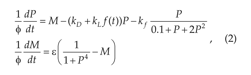
The Novak-Tyson Model

The NT model (Novak and Tyson, 2008; Tyson et al., 1999) for the molecular circadian clock in the fruit fly Drosophila contains 2 state variables representing mRNA concentration ( $M$ ) and protein ( $P$ ) concentration:

$$\begin{array}{l}\frac{1}{\mathrm{\varphi }}\frac{dP}{dt}=M-(k_D+k_{L}f(t))P-k_f\frac{P}{0.1+P+2P^2}\\ \frac{1}{\mathrm{\varphi }}\frac{dM}{dt}=\epsilon \left(\frac{1}{1+P^4}-M\right),\end{array}$$

where all parameters are positive. The $\mathcal{P}$ variable represents 2 proteins (PER and TIM) that form a heterodimer and create a negative feedback loop by inhibiting transcription of their own genes. The parameter $\epsilon$ is taken to be small, which creates a separation of time scales between the $P$ and $M$ variables. The parameter $\mathrm{\varphi }$ governs the rate of flow of trajectories in the phase plane and will directly affect the period of any solutions we find. The parameter $k_D$ is the baseline protein degradation rate during darkness. In Drosophila, light is known to increase degradation of TIM; $k_L$ is the added degradation rate due to light. The parameter $k_f$ captures the extent of positive feedback due to stabilization of the protein after dimerization. The function $f(t)$ describes the light stimulus. In complete darkness, $f(t)\equiv 0$ . In complete light, $f(t)\equiv 1$ . When the model is subjected to a periodic photoperiod, $f(t)$ is chosen to be a smooth cut-off version of a periodic step function that takes on the value $0$ during darkness and $1$ during light.

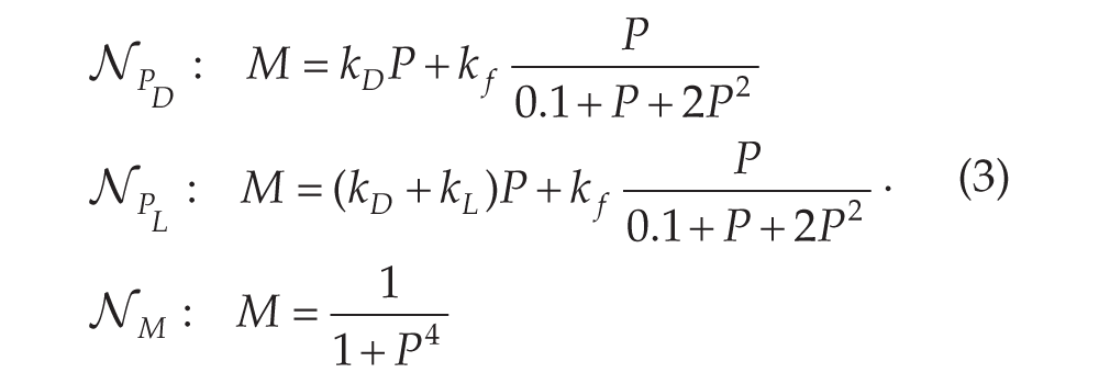
Consider first the situation of either constant darkness $f(t)\equiv 0$ , or constant light, $f(t)\equiv 1$ . In each case, the nullclines consist of the set of points where the right-hand sides of the equations in Equation (2) equal 0. In particular, we define $P$ -nullclines for each case together with a common $M$ -nullcline.

$$\begin{array}{l}{\mathcal{N}}_{P_D}:M=k_{D}P+k_f\frac{P}{0.1+P+2P^2}\\ {\mathcal{N}}_{P_L}:M=(k_D+k_L)P+k_f\frac{P}{0.1+P+2P^2}\\ {\mathcal{N}}_M:M=\frac{1}{1+P^4}.\end{array}$$

Both ${\mathcal{N}}_{P_D}$ and ${\mathcal{N}}_{P_L}$ form cubic shaped curves in the $P-M$ phase plane. We sometimes use the notation ${\mathcal{N}}_P$ to refer to the $P$ -nullcline when it does not matter whether we are referring to dark or light. The curve ${\mathcal{N}}_M$ is qualitatively sigmoidal shaped. Depending on where the $P$ and $M$ nullclines intersect, the ensuing fixed point(s) may be stable or unstable. Any intersection that occurs on the left or right branches of $P$ -nullclines are stable, while those that occur on the middle branch will be unstable provided that $\epsilon$ and $k_D$ are not too large. The standard set of parameters that we use for a single cell produces an unstable fixed point along the middle branch. In either constant darkness or constant light, it is straightforward to use dynamical systems methods to prove the existence of a stable limit cycle (periodic orbit) solution, as discussed in the Results section.

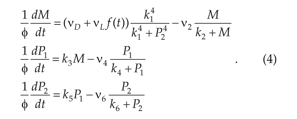
The Gonze Model and the Kim-Forger Model

We also consider 2 different models of the molecular circadian clock in mammals. The Gonze model (Gonze et al., 2005) is a modified version of the Goodwin oscillator (Goodwin, 1965) describing the core negative feedback loop of the circadian cock. There are 3 state variables that represent concentrations of mRNA ( $M$ ), protein ( $P_1$ ), and protein in its active form ( $P_2$ ) of a clock gene such as Per or Cry:

$$\begin{array}{l}\frac{1}{\mathrm{\varphi }}\frac{dM}{dt}=({\nu }_D+{\nu }_{L}f(t))\frac{k_1^4}{k_1^4+P_2^4}-{\nu }_2\frac{M}{k_2+M}\\ \frac{1}{\mathrm{\varphi }}\frac{d{P}_1}{dt}=k_{3}M-{\nu }_4\frac{P_1}{k_4+P_1}\\ \frac{1}{\mathrm{\varphi }}\frac{d{P}_2}{dt}=k_5{P}_1-{\nu }_6\frac{P_2}{k_6+P_2}.\end{array}$$

Specifically, $P_2$ is the nuclear form of PER/CRY that inhibits transcription of the clock gene. In mammals, light is known to increase the transcription rate of Per1 and Per2 (Golombek and Rosenstein, 2010); thus, we have included the LD forcing in the first term of the $dM/dt$ equation. The following parameter values were used: ${\nu }_D=0.7$ , ${\nu }_L=0.1$ , $k_1=1$ , ${\nu }_2=0.35$ , $k_2=1$ , $k_3=0.7$ , ${\nu }_4=0.35$ , $k_4=1$ , $k_5=0.7$ , ${\nu }_6=0.35$ , and $k_6=1$ .

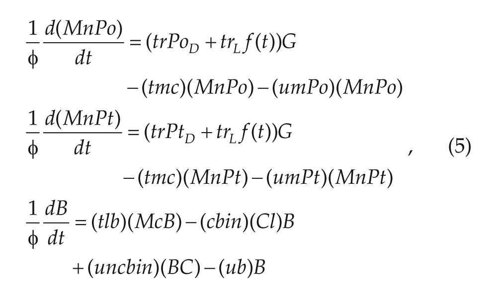
The Kim-Forger model contains the core negative feedback loop as well as additional secondary feedback loops. The model has 180 state variables representing nuclear and cytoplasmic concentrations of mRNA and protein products for several clock genes including Per1, Per2, Cry1, Cry2, Bmal, Npas2, and Rev-erb, as well as other regulatory elements. For a detailed description of the full model, see Forger and Peskin (2003) and Kim and Forger (2012). Here we only show the differential equations for the 2 state variables that receive LD forcing, which are Per1 and Per2 mRNA in the nucleus ( $MnPo$ and $MnPt$ ), and the state variable that we will use to define the entrainment map for this model, which is BMAL protein in the cytoplasm ( $B$ ):

$$\begin{array}{l}\frac{1}{\mathrm{\varphi }}\frac{d(MnPo)}{dt}=(trP{o}_D+t{r}_{L}f(t))G-(tmc)(MnPo)-(umPo)(MnPo)\\ \frac{1}{\mathrm{\varphi }}\frac{d(MnPt)}{dt}=(trP{t}_D+t{r}_{L}f(t))G-(tmc)(MnPt)-(umPt)(MnPt)\\ \frac{1}{\mathrm{\varphi }}\frac{dB}{dt}=(tlb)(McB)-(cbin)(Cl)B+(uncbin)(BC)-(ub)B\end{array},$$

where $G$ , $McB$ , $Cl$ , and $BC$ are state variables representing the probability of the E-box promoter being activated, Bmal mRNA and CLOCK/NPAS2 protein concentrations in the cytoplasm, and the concentration of unphosphorylated BMAL-CLOCK/NPAS2. The parameters $trP{o}_D$ and $trP{t}_D$ are basal transcription rate constants in darkness, $t{r}_L$ is additional transcription due to light, $umPo$ and $umPt$ are degradation rate constants, and $tmc$ is the rate constant for folding and nuclear export of mRNA. Finally, the parameters $tlb$ , $ub$ , $cbin$ , and $uncbin$ are rate constants for BMAL translation, BMAL degradation, and binding and unbinding of BMAL to CLOCK/NPAS2. We used the parameter values given in Kim and Forger (2012), with $trP{o}_D=25.9201$ , $trP{t}_D=44.854$ , and $t{r}_L=10$ .

For all 3 of these models, we will show via simulation that the 1-dimensional entrainment map yields accurate predictions for the phase of entrainment.

Effects of Sensory Input: Light and Darkness

We shall be interested in the response to 3 different scenarios: constant darkness, constant light, and periodic switching between the two with a prescribed photoperiod. We will show that over a wide range of parameters, the models produce stable periodic solutions in constant darkness, referred to as DD, or in constant light, denoted LL. We denote the “free-running” period of the DD oscillator as $\tau$ . In the case of periodic forcing, we follow a protocol that is often used in experiments. Namely, we will study the entrainment of oscillators to a periodic signal that models a photoperiod of a 24-h cycle consisting of an $N$ hour “light” interval (L) followed by a 24- $N$ hour “dark” interval (D). When an oscillator is subjected to a light-dark photoperiod (LD), depending on parameters, it may entrain to the 24-h forcing. By entrain we mean that the solution is periodic and that it has a period of 24 h. If these conditions are met, we call the ensuing periodic solution an LD-entrained solution.

To consider an oscillator subjected to periodic forcing of $N$ hours of light followed by $24-N$ hours of darkness, we allow $f(t)$ to vary periodically between 0 and 1. In our simulations, $f(t)$ is a rectangular wave with instantaneous transitions. When analyzing the periodically forced system, we consider $f(t)$ to be a smooth approximation of a rectangular wave.

The Entrainment Map $\mathrm{\Pi }(x)$

The entrainment map $\mathrm{\Pi }(x)$ is the primary tool we will use to understand the properties and consequences of phase-locking. To define $\mathrm{\Pi }(x)$ , we choose a Poincaré section $\mathcal{P}$ as an $n-1$ dimensional hyperplane that intersects a point on the LD cycle. To define a hyperplane, we only need to specify the value of 1 of the variables and the direction of the flow as it crosses the hyperplane. For example, in the 2-dimensional NT model, $\mathcal{P}$ is a 1-dimensional line segment that intersects the LD-entrained solution chosen along the left branch of ${\mathcal{N}}_P$ at $M=0.44$ where $dM/dt>0$ . This is a natural location to place $\mathcal{P}$ since the flow forces trajectories to enter a neighborhood of that branch. We note that the method still works if we choose $\mathcal{P}$ to lie along a different portion of the LD cycle, for example, away from the left branch, as discussed in the Supplementary Material, Section R2. In the Gonze and Kim-Forger models, there is no natural location to choose for the Poincaré section. We choose the section in these cases by specifying a variable that does not receive the light-dark forcing. For the 3-dimensional Gonze model, $\mathcal{P}$ is a 2-dimensional hyperplane chosen at $P_1=0.35$ where $d{P}_1/dt>0$ . For the 180-dimensional Kim-Forger model, $\mathcal{P}$ is a 179-dimensional hyperplane chosen at $B=20$ where $dB/dt>0$ . Assume that the oscillator has an initial condition lying on the Poincaré section. We define $x$ to be the amount of time that has passed since the beginning of the most recent LD cycle. When the trajectory is again on $\mathcal{P}$ , we define the map $\mathrm{\Pi }(x)$ to be the amount of time that has passed since the onset of the most recent LD cycle. The domain and range of $\mathrm{\Pi }(x)$ are the set $[0,24]$ . The domain is considered to be periodic, where $x=0$ and $x=24$ are equivalent. The Poincaré map relates the value of $x$ at one cycle to its value at the next; $x_{j+1}=\mathrm{\Pi }(x_j)$ for $j\ge 0$ . Unless otherwise noted, we limit our discussion of the properties of the map to parameter sets where both the LL and DD limit cycles exist. Details on how we conducted the numerical simulations to construct the map are provided in the Supplementary Material, Section M1.

The map $\mathrm{\Pi }(x)$ can be decomposed in the following way. Define a return map $\rho (x)$ that measures the time a trajectory starting on $\mathcal{P}$ , $x$ hours into an LD cycle, takes to return to $\mathcal{P}$ . Then $\mathrm{\Pi }(x)=\rho (x)+x\mathrm{mod}24$ . Because of the mod operation, it is not readily clear whether the trajectory returns to $\mathcal{P}$ in the same LD cycle in which it started or in a subsequent one. 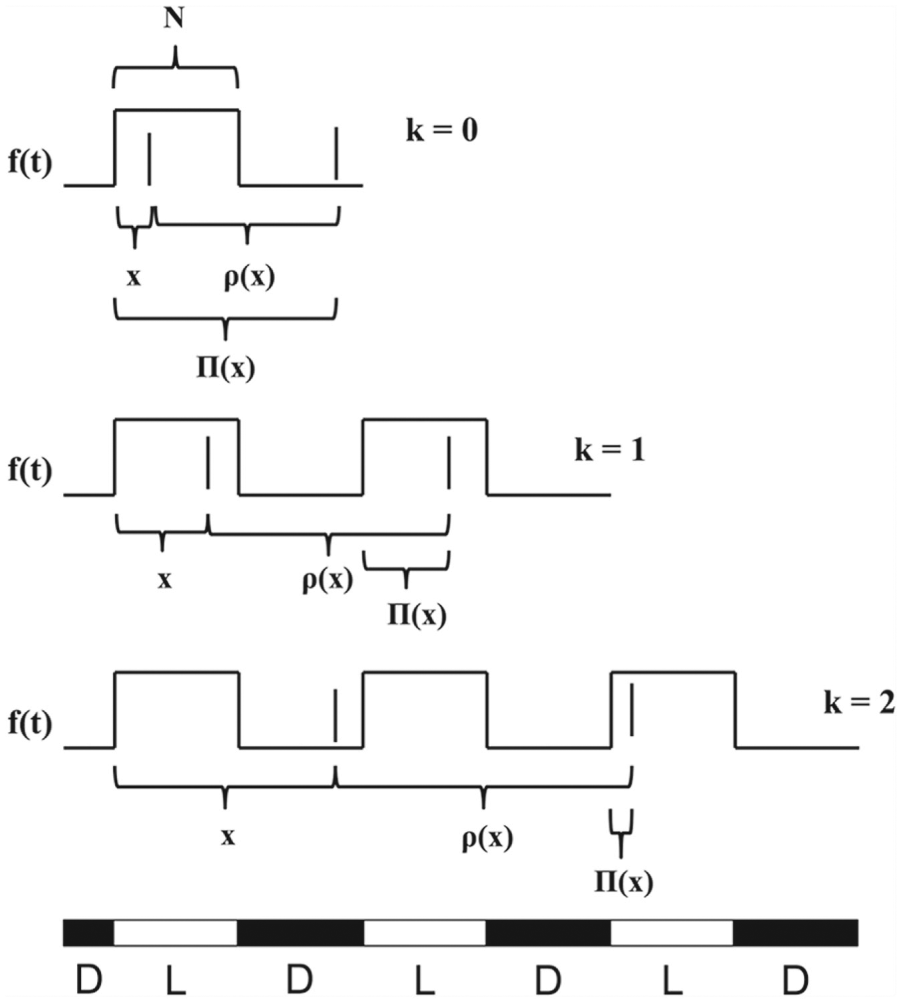To clarify this point, note that if $\rho (x)<24-x$ , the trajectory will return back to $\mathcal{P}$ within the same LD cycle in which it started. Thus, $\mathrm{\Pi }(x)=\rho (x)+x$ . If $24-x<\rho (x)<48-x$ , then the trajectory returns in the next LD cycle and $\mathrm{\Pi }(x)=\rho (x)+x-24$ . In general, we can write $24k<\rho (x)+x<24(k+1)$ , for $k=0,1,2,\dots$ and $\mathrm{\Pi }(x)=\rho (x)+x-24k$ . The case $k=0$ corresponds to the trajectory returning to $\mathcal{P}$ in the same LD cycle it started in, $k=1$ in the next cycle, $k=2$ in the subsequent cycle, and so on. See Figure 1 for an illustration.

Figure 1.

Schematic that defines $x$ , $\rho (x)$ , and $\mathrm{\Pi }(x)$ in various cases. In each panel, the solid vertical lines denote 2 consecutive moments in time when the oscillator crosses the Poincaré section $\mathcal{P}$ . The square wave denotes $f(t)$ , which varies between 0 and 1, and the LD photoperiod is shown at the bottom of the figure. The time $x$ is measured as the distance in time from the start of the first light pulse (when $f(t)$ increases to 1) to the first crossing of $\mathcal{P}$ , and $\rho (x)$ is the distance in time between crossings of $\mathcal{P}$ . The value $\mathrm{\Pi }(x)$ measures the distance in time from the start of the most recent onset of lights to the next crossing of $\mathcal{P}$ . The 3 panels shown correspond to the 3 possible scenarios that arise in defining the entrainment map.

The map $\rho (x)$ measures the time it takes a trajectory leaving $\mathcal{P}$ to return to it. It has a periodic domain $[0,24]$ , and its range lies in the set of positive numbers. It has several generic properties: $\rho (x)$ is continuous (since the forced vector field of Equation (2) is smooth), $\rho (x)$ is periodic at its endpoints $\rho {(0}^{+})=\rho {(24}^{-})$ (since the domain is periodic), and $\rho (x)$ is decreasing on a subinterval of its domain (as shown in the Results section).

A stable fixed point of the map $\mathrm{\Pi }(x)$ , denoted $x_s$ , corresponds to a one-to-one entrained solution and determines the phase of locking. A stable fixed point satisfies 2 conditions, $x_s=\mathrm{\Pi }(x_s)$ and $|{\mathrm{\Pi }}^{\prime }(x_s)|<1$ . Both conditions can be checked by plotting the map and determining whether and with what slope the graph intersects the diagonal. When a stable, phase-locked solution exists, the map $\mathrm{\Pi }(x)$ is ideally suited to calculate the time to approach the stable solution starting from any initial condition. If $x_s$ is a stable fixed point of the map and $\left\{x_j\right\}$ is a sequence of iterates of the map, we say that the solution is entrained if there exists $m$ , such that for all $j\ge m$ , $|x_s-x_j|<0.5$ . Given an initial condition $x_0$ , we use the map to determine $m$ and thereby determine the time to entrainment. We will show by comparison to direct simulations of the full system that this method is quite accurate.

There is a considerable amount of flexibility in how the Poincaré section is chosen. This is because of a basic theoretical result of smooth differential equations: namely, that solution trajectories depend continuously on initial conditions. To build the map $\mathrm{\Pi }(x)$ , for each $x$ , we start with an initial condition that lies on the intersection of $\mathcal{P}$ and the LD-entrained solution (e.g., in the Gonze model at the value $M=0.21$ , $P_1=0.35$ , and $P_2=1.73$ ). Because the value of $x$ is not necessarily the fixed point $x_s$ , the ensuing trajectory is not the entrained solution. But the theory of smooth dynamical systems guarantees that the solution trajectory will lie close to the LD-entrained solution for a finite amount of time. The terms close and finite can be made mathematically precise, but for our purposes it is enough to guarantee that the trajectory again crosses $\mathcal{P}$ in a neighborhood of the crossing point of the entrained solution. This basic theoretical fact is what allows the entrainment map to be constructed for high-dimensional models for which the LD-entrained solution has first been numerically computed. Different choices of the Poincaré section will lead to different entrainment maps. But for any choice, the ensuing LD-entrained solutions will all have the same phase of entrainment, as discussed in the Supplementary Material, Section R2.

The entrainment map is defined by setting $x=0$ as the reference phase with respect to the onset of lights in a 24-h light-dark cycle. This is in contrast to PRC-based methods, where the reference phase is typically assigned to a point along the DD oscillator. Although it may not seem that assigning the reference phase to a point on the underlying light-dark forcing instead of DD or LL makes much of a difference, we will show that doing so allows us to use information from the DD, LL, and LD-entrained solutions to construct the map. Additionally, the entrainment map allows the light pulse (or the dark pulse) to be split up so that it appropriately represents the relationship of the oscillator to the ongoing light-dark cycle and not just as a single pulse at a predetermined phase as in a PRC. As a result, we will show that for all the models we tested, the map ends up yielding a more accurate prediction about phase locking than the PRC.

Results

We begin by analyzing the NT model. Many of the details of the phase plane analysis can be found in the Supplementary Material. We then turn to the Gonze and Kim-Forger models and show that the entrainment map also works well in these higher-dimensional settings.

LD-Entrained Oscillations in the Novak-Tyson Model

When $f(t)\equiv 0$ , Equation (2) produces a limit cycle corresponding to a DD oscillator (black dashed curve in Fig. 2A). This stable limit cycle exists due a simple application of the Poincaré-Bendixson theorem. Namely, one can build a bounded, positively invariant region that surrounds the single fixed point that lies on the middle branch of ${\mathcal{N}}_M$ . Since this fixed point is unique and unstable, the Poincaré-Bendixson ensures the existence of a stable limit cycle. When $f(t)\equiv 1$ , the $P$ -nullcline shifts up in phase space, but the fixed point remains on the middle branch. Again the Poincaré-Bendixson theorem applies, proving the existence of the LL limit cycle (dashed red curve in Fig. 2A). Note that the DD limit cycle has a larger amplitude in the $\mathcal{P}$ direction. This is a consequence of the difference in the $P$ -nullcline between the DD and LL cases. Also note that the 2 limit cycles share a common fast-slow structure that allows them to largely overlap near the left branch of ${\mathcal{N}}_P$ . Indeed, as $\epsilon \to 0$ , Equation (2) becomes singularly perturbed and portions of the LL and DD trajectories would lie on the left and right branches of ${\mathcal{N}}_P$ . For any $\mathrm{\varphi }$ , the period of the LL limit cycle is less than that of the DD limit cycle (the opposite is true for the Gonze and Kim-Forger models, as discussed in the section on higher dimensional models). This is a result of the faster dynamics in the LL case due to ${\mathcal{N}}_{P_L}$ being higher in the phase space than ${\mathcal{N}}_{P_D}$ .

Figure 2.

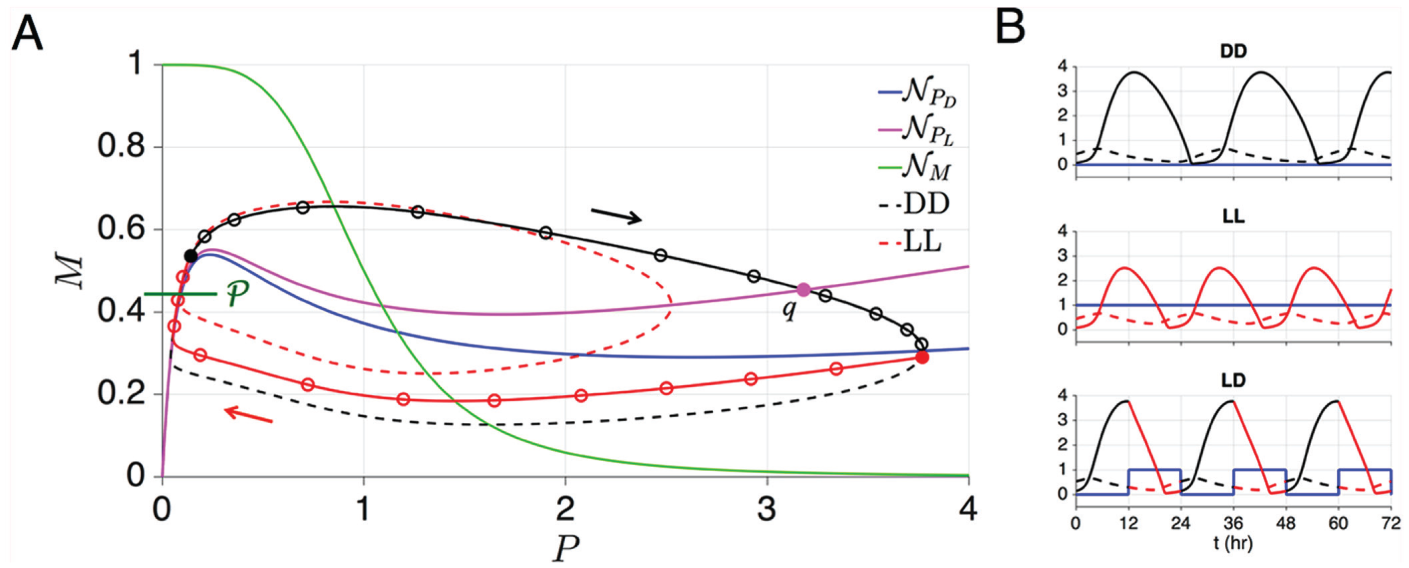
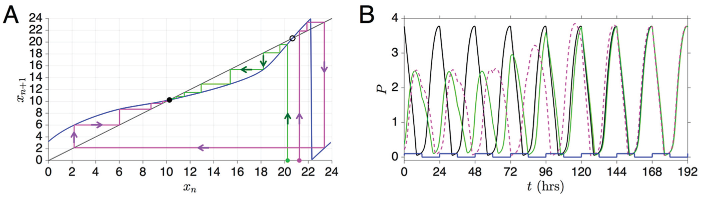
(A) The DD (dashed black), LL (dashed red) and LD (solid red-black) solutions of the NT model are shown in the phase plane. The LD-entrained solution overlaps the DD oscillator’s trajectory during darkness (black) and then deviates from it near $P=4$ when the lights turn on (red). Trajectories move clockwise in the plane. Open circles denote hourly intervals. The green horizontal line segment is $\mathcal{P}$ . The point $q$ is the intersection of the LD-entrained trajectory with ${\mathcal{N}}_{P_L}$ and is referred to in the Supplementary Material, Section R1. (B) Time courses of the $\mathcal{P}$ (solid) and $M$ (dashed) variables. The free-running period of the DD oscillator ( $f(t)\equiv 0$ [blue line], top trace) is longer than that of the LL oscillator ( $f(t)\equiv 1$ , middle trace). Entrainment to a 24-h periodic 12:12 forcing $f(t)$ (bottom trace) results in an LD-entrained oscillation.

In the presence of light-dark forcing, the ensuing trajectory spends its time in phase space approaching the DD cycle during darkness and the LL cycle during light. This idea was noted in earlier work by Peterson (1980) (Johnson et al., 2003; Pittendrigh, 1981). In some sense, the trajectory uses the stable structure of the DD and LL limit cycles to transiently approach the appropriate one during relevant time intervals. For this planar model, this back and forth serves to bound where in phase space the trajectory can lie at any moment in time. The LD-entrained solution is shown in Figure 2A. Note that the entrained solution tracks the DD limit cycle for a portion of its trajectory and then deviates from it near $P=3.7$ . From that point, the trajectory is attracted toward the LL limit cycle, although it reaches the left branch of the $P$ -nullcline prior to entering a neighborhood of the LL cycle. This is because the rate of attraction to the LL limit cycle is not overly large. Open circles along the LD-entrained solution denote hourly intervals. Figure 2B shows time traces of the DD, LL, and LD-entrained solutions. The latter additionally shows the relationship of the entrained solution to the light-dark pulse. For the parameters used in the simulation, the peak value of $M$ happens to occur near the beginning of the dark period. The entrainment map will help to explain why this is the case.

Let us consider a specific set of parameters referred to as the canonical set for the NT model ( $\mathrm{\varphi }=2.1,k_D=\mathrm{0.05,}{k}_L=0.05,k_f=1,\epsilon =0.05$ and a 12:12 photoperiod). Figure 3A shows an annotated phase plane of the LL and DD cycles for this set of parameters. On the respective cycles, solid dots depict hourly intervals. The total length of time of the LL cycle is 21.64 h, and that of the DD cycle is 28.9 h. The 2 cycles effectively overlap along the left branch of ${\mathcal{N}}_P$ . They also intersect near $P=1.5$ , $M=0.65$ . Call this point $c_p.$ To facilitate the construction of $\mathrm{\Pi }(x)$ , let us first consider $\rho (x)$ and explain why it has an interval of points on which it is decreasing. Let $x_L$ be the time it takes a trajectory to evolve along the LL cycle from $\mathcal{P}$ to $c_p$ and $x_D$ the time along $DD$ between these 2 objects. For the case of $\mathrm{\varphi }=2.1$ , $x_L=7$ and $x_D=6.3$ . Define $x_1=12-x_L$ and $x_2=24-x_D$ . Let us consider the trajectory that has initial condition x1 $x_1$ . This trajectory evolves along the LL cycle for $x_L$ until it reaches $c_p$ . At this point, the lights switch off and the trajectory now must follow the DD cycle for 12 h. The length of time of the DD cycle between $c_p$ and $\mathcal{P}$ is 22.6 h. Thus, when the lights turn back on, the trajectory is very far from $\mathcal{P}$ . In contrast, the trajectory with initial condition $x_2$ travels for $x_D$ hours on DD to $c_p$ . From here it travels 12 h on the LL cycle. The length of time on LL from $c_p$ to $\mathcal{P}$ is 14.6 h. Thus, after 12 h on LL, the trajectory is very close to $P.$ If $r(x_i)$ denotes the remaining time for each trajectory to reach $\mathcal{P}$ , it is clear that $r(x_1)>r(x_2)$ . Given that $x_L$ is close to $x_D$ , it follows that $\rho (x_1)>\rho (x_2).$ The continuity of $\rho (x)$ then implies there must be a subinterval of $(x_1\mathrm{,}{x}_2)$ on which $\rho (x)$ is decreasing. Note that the actual interval on which $\rho (x)$ is decreasing may in fact contain $(x_1\mathrm{,}{x}_2)$ rather than be contained in it. Because of periodicity, $\rho (x)$ must also be increasing over a different interval(s). Figure 3B shows $\rho (x)$ for the case $\mathrm{\varphi }=2.1$ . Note that the curve is qualitatively a cubic with a single interval over which it is decreasing. This interval contains $(x_1\mathrm{,}{x}_2)$ . Since $\rho (x)$ is continuous on a closed interval, it attains its maximum and minimum values. It is fairly easy to get a bound on these values. The upper bound is attained near $x_1$ and is obtained by taking the LL cycle from $\mathcal{P}$ to $c_p$ and the DD cycle from $c_p$ back to $\mathcal{P}$ . This yields a time of 29.6 h. The lower bound occurs near $x_2$ and is obtained by taking DD from $\mathcal{P}$ to $c_p$ , then LL back to $\mathcal{P}$ , yielding a time of 20.9 h. This yields a bound on $d\rho (x)/dx$ on $(x_1\mathrm{,}{x}_2)$ as $(20.9-29.6)/(17.7-5)=-0.71>-1$ . Note from Figure 3B that along the decreasing portion, there exists a unique value $x_s\in (x_1\mathrm{,}{x}_2)$ for which $\rho (x_s)=24$ . There is also another value $x_u$ along the increasing portion of $\rho (x)$ for which $\rho (x_u)=24$ . Although it is obvious from our simulation results that $x_s$ and $x_u$ exist, analytically proving this fact is beyond the scope of this paper.

Figure 3.

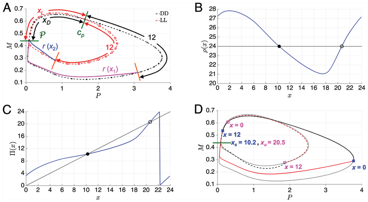
(A) DD (dashed black) and LL (dashed red) limit cycles with open circles indicating hourly intervals starting at $\mathcal{P}$ . $c_p$ is an intersection point of these 2 limit cycles. Times along the DD and LL limit cycles between $\mathcal{P}$ and $c_p$ are indicated as x_D and x_L. The orange lines are located 12 h in time along the DD and LL limit cycles from the point $c_p$ . The times $r(x_1)=8.16$ h and $r(x_2)=2.74$ h are numerically computed as the remaining time it takes the respective trajectories (magenta and blue) to return to $\mathcal{P}$ . (B) Numerically computed $\rho (x)$ . Solid and open dots depict $x_s$ and $x_u$ . (C) Numerically computed $\mathrm{\Pi }(x)$ . Solid and open dots depict crossings with the diagonal and correspond to the stable and unstable phase locked solutions $x_s$ and $x_u$ . (D) Stable (solid) and unstable (dashed) LD limit cycles corresponding to $x_s$ and $x_u$ . The LL (light gray, smaller amplitude) and DD (light gray, larger amplitude) solutions are shown for comparison.

In Figure 3C, we show the graph of the map $\mathrm{\Pi }(x)$ . Note that $x_s$ and $x_u$ are fixed points of this map. Further, ${\mathrm{\Pi }}^{\prime }(x)={\rho }^{\prime }(x)+1>0$ since $-1<{\rho }^{\prime }(x)$ , implying that the graph of $\mathrm{\Pi }$ is increasing wherever it is continuous. It has a discontinuity whenever $\rho (x)+x$ passes through a multiple of 24. Finally, note that $|{\mathrm{\Pi }}^{\prime }(x_s)|<1$ , implying that $x_s$ is a stable fixed point, whereas ${\mathrm{\Pi }}^{\prime }(x_u)>1$ , implying that $x_u$ is an unstable fixed point. The stable fixed point $x_s$ corresponds to a stable LD-entrained solution and is shown in Figure 3D. The stable fixed point occurs at $x_s=10.2$ , which means that when the LD-entrained solution starts on $\mathcal{P}$ , it initially experiences 1.8 h of light. This is followed by 12 h of darkness, where the trajectory tracks the DD limit cycle. After this time, the trajectory is again subject to conditions of light, and it can be seen that the trajectory deviates from the DD limit cycle. Similarly, $x_u$ corresponds to an unstable LD-entrained solution, which is also shown in Figure 3D. The value $x_u=20.5$ , so it initially experiences about 3.5 h of darkness when starting on $\mathcal{P}$ before then experiencing 12 h of light and then subsequent darkness. In some sense, for this set of parameters, its trajectory experiences light and darkness at opposite locations in phase space relative to the solution associated with $x_s$ . Further consequences of the existence of $x_s$ and $x_u$ are explored below when we discuss the dynamics of entrainment.

Dependence of $\mathrm{\Pi }(x)$ on Parameters

To study how the map depends on parameters, we start with the canonical set of parameters and systematically vary one at a time. We begin with the parameter $\mathrm{\varphi }$ , which determines the intrinsic period of the oscillator by controlling the rate of evolution of both the $P$ and $M$ variables. Larger $\mathrm{\varphi }$ implies a faster oscillator. If $\mathrm{\varphi }$ is too large, however, then the intrinsic period of the circadian clock is too small (much less than 24) and phase-locking with a 24-h forcing will not be possible. The same conclusion occurs when $\mathrm{\varphi }$ is too small and the circadian clock is too slow. Thus, there exists an interval $({\mathrm{\varphi }}_{min}\mathrm{,}{\mathrm{\varphi }}_{max})$ such that stable one-to-one entrainment occurs for $\mathrm{\varphi }$ lying in that interval. This is a standard result from the forced oscillator literature; see Glass (1991) for an example.

Supplementary Figure S1 shows that $\rho (x)$ shifts down when $\mathrm{\varphi }$ is increased. This makes sense as faster dynamics imply smaller transit times and so $\rho (x)$ should be smaller. In addition, $\rho (x)$ also shifts to the right, as explained in the Supplementary Material, Section R1. Figure 4A shows the map $\mathrm{\Pi }(x)$ for several different choices of φ $\mathrm{\varphi }$ . As φ increases, the curves shift down and to the right, the discontinuity moves to the right, and the stable fixed point $x_s$ moves down and to the left. Biologically, this means that faster intrinsic oscillators encounter light earlier in the subjective day when entrained than do slower intrinsic oscillators. In other words, fast intrinsic oscillators have advanced phases of entrainment (morning larks) and slow intrinsic oscillators have delayed phases of entrainment (night owls) (Bordyugov et al., 2015). Note that as $\mathrm{\varphi }$ increases, the value of $x_s$ increases from around 5 h at $\mathrm{\varphi }=1.865$ to 15 h at $\mathrm{\varphi }=2.506$ . The value ${\mathrm{\varphi }}_{min}=1.865$ corresponds to the saddle node bifurcation where the map lies above and tangent to the diagonal; ${\mathrm{\varphi }}_{max}=2.506$ corresponds to a second saddle node bifurcation that occurs when the map lies below and tangent to the diagonal. The interval $({\mathrm{\varphi }}_{min}\mathrm{,}{\mathrm{\varphi }}_{max})$ is called the $\mathrm{\varphi }$ -range of entrainment. To understand the path through which entrainment is lost, note that as $\mathrm{\varphi }$ approaches ${\mathrm{\varphi }}_{min}$ from above or ${\mathrm{\varphi }}_{max}$ from below, the fixed points $x_s$ and $x_u$ merge in a saddle-node bifurcation. This merging corresponds to a saddle-node bifurcation of periodic orbits in phase space, as described in Supplementary Material, Section R1.

Figure 4.

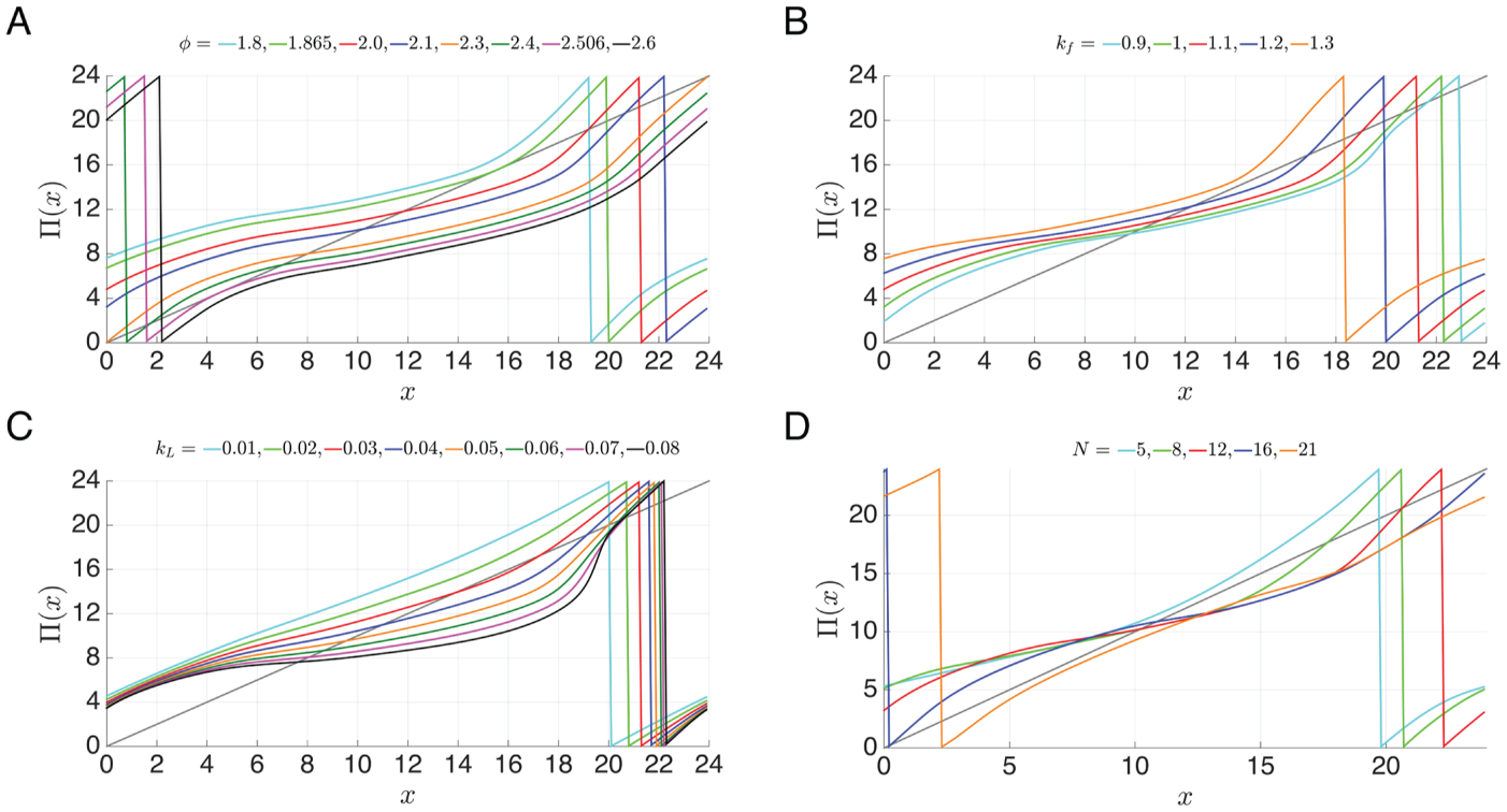
The entrainment map $\mathrm{\Pi }(x)$ changes systematically as intrinsic (A, B) and extrinsic (C, D) model parameters are varied. (A, B) Increasing the intrinsic speed of oscillators by (A) increasing $\mathrm{\varphi }$ or (B) decreasing $k_f$ moves the stable fixed point of the map to the left and leads to entrained oscillators that encounter light earlier in the subjective day. Loss of entrainment occurs when the curves do not intersect the diagonal. (C) Increasing $k_L$ also moves the stable fixed point of the map to the left, corresponding to increased light intensity advancing the phase of entrainment. The increased concavity of $\mathrm{\Pi }(x)$ as $k_L$ increases suggests that brighter light decreases the amount of time required to reach stable entrainment. (D) Changes in light duration ( $N$ ) have only a minor effect on the location of the stable fixed point of the map, suggesting that the photoperiod does not significantly affect the phase of entrainment for these parameter values. However, the fixed points do undergo saddle-node bifurcation if the light duration is too short or too long, corresponding to loss of entrainment in extreme photoperiods.

The parameter $k_f$ is associated with positive feedback in the accumulation of protein due to inhibition of protein degradation (Novak and Tyson, 2008; Tyson et al., 1999). Increasing $k_f$ moves the $P$ -nullcline up in the phase space. However, this effect is much more pronounced on the left branch of the $P$ -nullcline. As a result, the dynamics slow down near the left branch, more than they speed up away from it, resulting in a net slower speed. This causes $\mathrm{\Pi }(x)$ to shift up and to the left and the stable fixed point $x_s$ to move down and to the right (Fig. 4B). Thus, increasing the amount of positive feedback slows down the intrinsic oscillations (consistent with recent findings in other circadian models; Ananthasubramaniam and Herzel, 2014) and leads to entrained clocks encountering light later in the subjective day. When $k_f$ increases to 1.27, the fixed points $x_s$ and $x_u$ merge at a saddle node bifurcation, indicating that too much positive feedback can lead to loss of entrainment. As $k_f$ decreases, the fixed point along the middle branch of ${\mathcal{N}}_P$ eventually becomes stable, causing the disappearance of the LL oscillation at $k_f=0.88$ and DD at $k_f=0.70$ . Note, however, that for $0<k_f<0.88$ , even though we no longer have self-sustained LL and DD oscillations, it is still possible for the system to be driven by the forcing to exhibit 24-h rhythms. Mathematically, this occurs because in this range of $k_f$ , the model reduces to driving a stable fixed point with the 24-h forcing. The ensuing limit cycle is relatively small in amplitude and lies in a neighborhood of the intersection of the ${\mathcal{N}}_P$ and ${\mathcal{N}}_M$ nullclines. From a circadian point of view, this is an example of “masking” rather than entrainment (Mrosovsky, 1999).

Understanding the effect of changes in $k_L$ and $N$ is somewhat more complicated than the changes due to $\mathrm{\varphi }$ and $k_f$ . The reason is that changes in $k_L$ dramatically affect the right branch of ${\mathcal{N}}_{P_L}$ , while changes in $N$ affect where in phase space the LD-entrained oscillator experiences conditions of light or dark. As a result, their respective effects on the speed of the LD-entrained oscillator are less uniform than with the intrinsic parameters.

Increases in light intensity are modeled by increasing $k_L$ . For small values of $k_L$ , entrainment is not possible, since the forced oscillator will still be too slow. Thus, there is a minimum strength of $k_L=0.029$ needed to entrain. Over a range of values, increasing $k_L$ speeds up the oscillations, since in general, the dynamics under lights are faster than during dark. Figure 4C shows the effect of changing $k_L$ on the map $\mathrm{\Pi }$ . Because increases in $k_L$ speed up the dynamics, the map shifts down and to the right (although there is small region near $x=20$ where this is not true for the larger values of $k_L$ ) and the stable fixed point moves to the left. This corresponds to increased light intensity advancing the phase of entrainment. With our canonical parameter set, the intrinsic oscillator has a long DD period ( $\tau >24$ ) and a delayed phase of entrainment (i.e., a night owl). Thus, this result is consistent with the use of bright light therapy to treat patients with delayed sleep phase syndrome (Dodson and Zee, 2010). For this figure, we had to lower the Poincaré section to $M=0.4$ to guarantee that for any initial condition of the map, the ensuing trajectory crossed $\mathcal{P}$ in the first cycle of its oscillation. Note that this results in $x_s=9.76$ and $x_u=20.0$ for the canonical case. Increased values of $k_L$ cause the linear portion of the equation that determines ${\mathcal{N}}_{P_L}$ to dominate. In this case, ${\mathcal{N}}_{P_L}$ can become monotone increasing and nearly linear, which produces a stable fixed point at the intersection of ${\mathcal{N}}_M$ for $k_L=0.089$ . Thus, the LL limit cycle will fail to exist. Observe that for $k_L>0.089,$ although the LL oscillation fails to exist, the LD-entrained solution will continue to exist. For this case, during the light portion, the trajectory tracks the left branch of ${\mathcal{N}}_{P_L}$ toward the stable fixed point. This fixed point prohibits the trajectory from leaving ${\mathcal{N}}_{P_L}$ and, as a result, puts an upper bound on how fast the oscillator can evolve. When the lights turn off, the nullcline switches to ${\mathcal{N}}_{P_D}$ , which is cubic shaped, and the trajectory circles the unstable intersection point of ${\mathcal{N}}_{P_D}$ and ${\mathcal{N}}_M$ before returning the left branch of ${\mathcal{N}}_{P_D}$ . Thus, for arbitrarily large values of $k_L$ , oscillations persist, such that increasing the intensity of light can speed up the oscillations only to a certain extent and never too fast to disrupt entrainment.

Figure 4D shows how the map Π(x) depends on the photoperiod $N:24-N$ (LD). Increasing $N$ means that the oscillator is exposed to more light. Generally, this does speed up the dynamics. This fact is reflected by the discontinuity $x_d$ moving to the right as $N$ increases, similar to how it moves for all the other parameter variations that speed up the dynamics. What differs with changes in $N$ from other cases is that the map as a whole does not shift down and to the right. Entrainment continues to disappear through saddle node bifurcations if the LD forcing is too heavily skewed toward either the light or dark intervals. When $N$ is large, the photoperiod contains too long an interval of light. The oscillator becomes too fast and loses the ability to entrain in the same way that entrainment is lost when $\mathrm{\varphi }$ increases. In particular, the left part of the map $\mathrm{\Pi }(x)$ shifts down and to the right with increases in $N$ just as it does with increases in $\mathrm{\varphi }$ . The right part of the map shifts up when $N$ is decreased and the dark interval dominates. In that case, the oscillator eventually becomes too slow to entrain, similar to when $\mathrm{\varphi }$ is decreased. Further details explaining why the map behaves in this way are provided in the Supplementary Material, Section R1.

Dynamics of Entrainment

Having understood the situations that lead to the existence of the LD-entrained stable and unstable solutions, let us now turn to understanding some aspects of the transient dynamics of trajectories that start with initial conditions that lie off of these limit cycles. The most straightforward way to do this is to use the map $\mathrm{\Pi }$ to track the transient dynamics associated with an initial condition $x_0$ . This will allow us to make comparisons to a direct simulation in which we start an oscillator on the Poincaré section $\mathcal{P}$ , $x_0$ hours into an LD cycle.

For the map $x_{n+1}=\mathrm{\Pi }(x_n)$ , a cobweb diagram from any initial condition x₀ ≠ x_u $x_0\ne x_u$ shows that the trajectory converges to the stable fixed point $x_s$ . We can readily determine 2 characteristics of entrainment: the time to entrainment and the direction of entrainment. In the Methods section, we defined a solution to be entrained if there exists $m$ , such that for all $j\ge m$ , $|x_s-x_j|<0.5$ . The integer $m$ depends on $x_0$ and refers to the number of iterates needed for the condition to hold from any given initial condition $x_0$ . We can calculate the time to entrainment in the following way. In the cobweb diagram, at each iterate, the trajectory hits either the upper or lower branch of $\mathrm{\Pi }$ . Let $x_d$ denote the value of the discontinuity of the map. Depending on the location of the discontinuity $x_d$ , the time $\rho (x)$ associated with that iterate will differ (see the Supplementary Material, Section R2, for details). The direction of entrainment refers to whether the cobwebbed iterate moves to the left or the right. When $x_{n+1}>x_n$ , then the iterate moves to the right, and the phase of the oscillator with respect to the onset of the lights is larger. Thus, we call this a phase delay. Alternatively, we obtain a phase advance when the iterate moves to the left when $x_{n+1}<x_n$ . Note, however, that transitions between branches follow a different rule. If $x_d>12$ , then a transition from the lower branch at one iterate to the upper branch at the next iterate is considered a phase delay, even though $x_{n+1}<x_n$ . This is because this type of iterate is equivalent to more than 24 h passing before the return to $\mathcal{P}$ . If $x_d<12$ , then the transition from upper branch to lower branch is considered a phase advance even though $x_{n+1}>x_n$ , since this type of iterate implies 2 crossings within one 24-h cycle. Finally, observe that the unstable fixed point $x_u$ demarcates which initial conditions lie on trajectories that entrain through phase advancing or phase delaying.

To study a specific example, we return to the map associated with the canonical set of parameters. Here $x_s=10.2$ , $x_u=20.5$ , and $x_d>12$ . Let us choose an initial condition $x_0=20.2$ . This point lies to the left of $x_u$ , so under the cobweb dynamics, it will move to the left and converge to $x_s$ from above, thereby phase advancing (green trajectory of Fig. 5A). Comparing to direct simulations, we find that the entrainment time is $158.281$ (6.6 days), which matches very well with the predictions of the map (157.247 h). As another example, choose $x_0=21.2$ , which lies to the right of $x_u$ . Now the iterates of the map move to the right, hit the lower branch of $\mathrm{\Pi }$ , and then are cobwebbed back to a smaller value of $x$ , from where they continue moving right (magenta trajectory in Fig. 5A). In this case, the oscillator entrains through phase delaying. From the map, we find the entrainment time to be 180.775 h (7.5 days) and from direct simulations to be 180.767 h. In Figure 5B, we show the time traces for solutions with each of these 2 initial conditions. Note that the green trajectory phase advances, while the magenta trajectory phase delays, consistent with the predictions of the map. Explicit values calculated from iterates of the map and direct simulations are shown in Tables S1 and S2 in the Supplementary Material, Section R2.

Figure 5.

Entrainment maps systematically reveal entrainment dynamics such as whether entrainment will occur through phase advances or phase delays. (A) Cobweb diagram showing convergence to $x_s$ starting from 2 different initial conditions $x_0=20.2$ (green trajectory) and $x_0=21.2$ (magenta trajectory). The former entrains by phase advancing, the latter by phase delaying. (B) The approach to the stable cycle shown in the $t$ versus $\mathcal{P}$ plane. Green and magenta traces correspond to the same values as in part A.

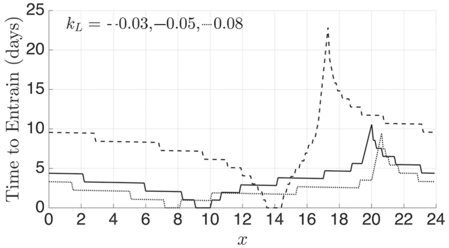
The map allows us to easily calculate entrainment time for any initial condition, for a range of parameters. For example, to see how light intensity affects entrainment time, we varied the initial conditions between 0 to 24 for 3 different values of $k_L$ ; see Figure 6 (also see the Supplementary Material, Section R2, which shows how choosing a different Poincaré section affects entrainment time). The solid curve denotes the canonical case $k_L=0.05$ , while the dashed and dotted curves are for $k_L=0.03$ and $0.08$ , respectively. As expected, for each curve, initial conditions that start in a neighborhood of $x_s$ (local minima of curve) take no time to entrain, while those in a neighborhood of $x_u$ take the longest. Note that $x_s$ and $x_u$ change as a function of $k_L$ , as can be seen from Figure 4C. Further note that stronger light $(k_L=0.08)$ leads, on average, to the shortest entrainment times, as can be observed by noting that the dotted curve lies on average below the others. This result can be predicted based on how the shape of $\mathrm{\Pi }(x)$ changes with $k_L$ . Observe from Figure 4C that as $k_L$ increases, the map has a region where the slope becomes smaller (roughly between $x=4$ and $x=16$ ) and a region where the slope and concavity increase (roughly between $x=16$ and $x=20$ ). It is in the region $x=10$ to $20$ that entrainment time dramatically decreases for $k_L=0.08$ . The reason is that iterates of the map use this sharp change in slope to make bigger advances toward the fixed point. This suggests that the amount of time required for a circadian oscillator to reentrain following a phase shift in the light-dark cycle, for example, after rapid transmeridian travel, will depend on light intensity with brighter light resulting in less jetlag.

Figure 6.

Time to entrain depends on light intensity and the proximity of initial phase to the stable and unstable fixed points. Larger values of $k_L$ , on average, lead to faster entrainment. For each case, the minimum entrainment time of 0 occurs for initial conditions in a neighborhood of $x_s$ and the maximum in a neighborhood of $x_u$ ( $x_s=13.9,9.5,7.6$ and $x_u=17.2,20.0,20.6$ for $k_L=0.03,0.05,0.08$ , respectively).

Relating $\mathrm{\Pi }(x)$ to a PRC

The phase response curve of an oscillator measures the change in asymptotic phase experienced when a perturbation is given to an oscillator along different parts of its limit cycle. In the context of our problem, we shall construct the PRC using a light pulse of length $N$ hours with $k_L=0.05$ . Specifically, start with a DD oscillator on the Poincaré section $\mathcal{P}$ . Allow it to evolve for $y$ hours along the DD limit cycle and then perturb it by introducing a light pulse of $N$ hours. We define

$$Z_k(y)=k\tau -{\tau }_k(y),$$

where $\tau$ is the free running period of the DD oscillator and ${\tau }_k(y)$ is the time when the perturbed oscillator crosses $\mathcal{P}$ for the $k$ th time. At each cycle, the quantity $Z_k(y)$ measures the deviation of the transit time of the perturbed oscillator from the DD oscillator. $Z_k(y)$ is often called the $k$ th-order PRC. Here, phase 0 is chosen as a point on the DD oscillator and thus the perturbed phase is defined relative to the DD oscillator itself. In general, such PRCs are typically used when 2 conditions are met: The duration $N$ of the light pulse is small, and the magnitude $k_L$ is not too large. These conditions imply that the effect of the light pulse is felt within the current or subsequent cycle to when it is applied and that the oscillator returns quickly to its intrinsic limit cycle thereafter, albeit with a potentially different phase. Both in theory and, as we will show, in practice, these conditions limit the applicability of using PRCs to determine phase-locking.

The map $\mathrm{\Pi }(x)$ can be directly compared to $Z_k(y)$ provided that both functions have the same domain. First, note that the domain of $Z_k$ is the interval $[0,\tau ]$ , while the domain for $\mathrm{\Pi }$ is $[0,24]$ . Thus, the 2 functions can be compared only when $\tau =24$ or by truncating the domain of $Z_k$ (if $\tau >24$ ) or $\mathrm{\Pi }$ (if $\tau <24$ ). To consider a case of $\tau =24$ , we set $\epsilon =0.01$ and $\mathrm{\varphi }=8.07$ . In turn, this implies that ${\tau }_1(y)=\rho (x)$ and $x+y=24$ , as shown in Figure S3 of the Supplementary Material, Section R3. Substitute into Equation (6) for $k=1$ to obtain

$$Z_{\mathrm{\Pi }}(y)=\tau -\rho (24-y).$$

The subscript on the PRC in this case indicates that this function is obtained from our map $\mathrm{\Pi }$ rather than directly through simulation. Additionally, it is convenient to leave $Z_{\mathrm{\Pi }}(y)$ expressed in terms of $\rho (24-y)$ rather than in terms of $\mathrm{\Pi }$ so that we can avoid the mod operation.

In Figure 7A, we show the results of directly computing the PRCs $Z_1(y)$ and $Z_2(y)$ for $N=1$ and $\tau =24$ with the map-based PRC $Z_{\mathrm{\Pi }}(y)$ . Note that because the effect of a single light pulse wears off relatively quickly, $Z_{k+1}(y)=Z_k(y)$ for $k\ge 2$ . A stable phase-locked solution will occur where the PRC has a root with negative slope. All 3 PRCs quantitatively agree with one another, although it is difficult to discern that the PRC is non-zero for small and large values of $y$ . In Figure 7B, we show the results for a case where the duration of the light pulse is not small, specifically $N=12$ . Note here that $Z_1(y)$ , $Z_2(y)$ , and $Z_{\mathrm{\Pi }}(y)$ differ quantitatively for larger values of $y$ . In particular, all 3 have different stable roots. By comparison to direct simulations, the roots predicted by $Z_1(y)$ and $Z_2(y)$ are incorrect, whereas the root predicted by the map-based $Z_{\mathrm{\Pi }}(y)$ is correct.

Figure 7.

The PRC fails to accurately predict the phase of entrainment for long light pulses, whereas the entrainment map is accurate for light pulses of any length. (A) For a short light pulse ( $N=1$ ), $Z_1$ , $Z_2$ , and $Z_{\mathrm{\Pi }}$ all agree with one another. (B) For a longer light pulse ( $N=12$ ), only $Z_{\mathrm{\Pi }}$ correctly predicts the value of the root computed by direct simulation (solid dot at $y=18.522$ ).

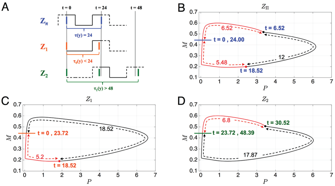
The preceding example of $N=12$ allows us to illustrate the primary difference between the entrainment map $\mathrm{\Pi }$ and the PRC, as well as the limitations of the latter. In Figure 8A, we show schematic diagrams of the case where $y$ is chosen as the root of $Z_{\mathrm{\Pi }}(y)$ ( $y=18.522$ ), which depicts where in time the oscillator is subjected to light. Figures 8B, 8C, and 8D show trajectories in the phase plane. In Figure 8A, the first solid line of each schematic denotes $t=0$ and represents the trajectory starting on the Poincaré section $\mathcal{P}$ . For the map $\mathrm{\Pi }(x)$ , $x=24-y$ is small (since $y$ is large), and thus the trajectory starts out with the lights on. In the phase plane, the trajectory will follow the LL cycle for $12-x$ hours, before then following the DD dynamics for 12 h. After that time, the trajectory will again be subjected to light during the remaining time $x$ it takes to return back to $\mathcal{P}$ . Thus, when constructing the entrainment map $\mathrm{\Pi }$ , the light pulse is allowed to be split up over different portions of the cell’s trajectory, as shown in Figure 8B. In contrast, when constructing the PRCs $Z_1(y)$ and $Z_2(y)$ , the light pulse is never split up. In the phase space, the trajectory now traverses along DD for $y$ hours before the lights turn on. Thus, in comparison to the $\mathrm{\Pi }$ -based trajectory, it is in a very different location in phase space when the LL dynamics come into play. The first crossing of $\mathcal{P}$ yields $Z_1(y)$ . As can be seen from Figure 8C, the oscillator has received only a small portion of the light pulse to this point, but it receives the light in a region of phase space that speeds up its oscillation. The second solid orange line in Figure 8A shows where the oscillator is relative to the light cycle at the moment it again crosses $\mathcal{P}$ . The light gray lines show 24-h intervals and represent where the oscillator would have been in the absence of light input. Thus, $Z_1(y)>0$ . After this point, the trajectory receives the remaining portion of light shown in Figure 8D but is actually in a region of phase space where the added light slows it down (lower schematic of Fig. 8A). In fact, it is slowed down so much that at the second crossing of $\mathcal{P}$ , $Z_2(y)<0$ .

Figure 8.

Comparison of how the light pulse affects the calculation made by the various PRCs. (A) Schematic showing where in time the oscillator crosses $\mathcal{P}$ (solid blue, orange, and green) and where the reference oscillator does for $Z_1$ and $Z_2$ (solid gray). The portion of the light pulse that is used in the calculation is shown in solid in each case. (B-D) Each panel shows where in phase space the light pulse affects the oscillator. (B) Effect of light pulse is split up in time, $t=0$ to $t=6.52$ , and then again from $t=18.52$ to $t=24$ . (C) The light pulse is only felt at the end of the oscillation from $t=18.52$ to $t=23.72$ . (D) The light pulse is only felt during $t=23.72$ to 30.52 $30.52$ .

When the intrinsic period of the DD oscillator is different than 24 h, then we must restrict the domain of $Z_k(y)$ or $\mathrm{\Pi }(x)$ to be able to directly compare them. Alternatively, we can simply compare the predictions regarding the phase of locking made by the map $\mathrm{\Pi }(x)$ versus those made by either $Z_1(y)$ or $Z_2(y)$ . We did so over a set of $\mathrm{\varphi }$ values (from $\mathrm{\varphi }=5.5$ to 8.25, with $\epsilon =0.01$ ) that span a range of intrinsic periods $\tau$ from 23.5 to 35.2. In all cases, when compared to direct simulations, the predictions made by the map $\mathrm{\Pi }$ were more accurate than those made via the PRCs; for details, see Table S3 in the Supplementary Material, Section R3. We also checked the accuracy of the predicted phase of entrainment for an alternative PRC construction protocol that was based on detecting peaks of the P variable rather than crossings of a Poincaré section. Specifically, we perturbed the canonical DD oscillator ( $\mathrm{\varphi }=2.1,\epsilon =0.05$ ) with light pulses ( $k_L=0.05$ ) and then measured the phase shift of the peak time in the sixth cycle after the perturbation. The PRC predicted the entrained phase correctly (within 2-min accuracy) for $N=12$ but was off by more than 30 min for $N=16$ . In contrast, the entrainment map predicted the entrained phase correctly (within 1 second accuracy) in both cases.

Higher Dimensional Models

We now show that the entrainment map can be defined in higher dimensional settings by constructing maps for the Gonze and Kim-Forger models. In each of these cases, the Poincaré section is chosen at a fixed value of a variable that does not receive the light-dark forcing $f(t)$ as described in the Methods section. Note that in addition to being of different dimensionality, these models also differ in the manner in which light enters the equations. In the fly model (NT), light increases the rate of protein degradation, whereas in the mammalian models (Gonze and Kim-Forger), light increases the rate of mRNA transcription. These distinct effects of light lead to contrasting relationships between DD and LL dynamics across the models. Specifically, the LL limit cycle has a shorter period than the corresponding DD limit cycle in the NT model but a longer period than the corresponding DD limit cycle in the Gonze and Kim-Forger models. Despite these differences in the behavior of these models under constant dark and constant light conditions, we find that the entrainment maps for these models share some common features and are able to accurately capture the effects of light-dark forcing in all 3 cases.

Figures 9A and 9B show the entrainment maps for 3 different values of the intrinsic periods of the respective models. Although it is difficult to see, note that as the intrinsic oscillator speeds up (increasing $\mathrm{\varphi }$ ), the maps move the same way as they did in the NT model. Namely, the entrained phase shifts to an earlier part of the light-dark cycle. The maps for both models also share with the NT maps the property of having 1 point of discontinuity. This commonality across the 3 models, together with those discussed below, suggests that the entrainment map provides a robust method for finding universal properties of circadian oscillators.

Figure 9.

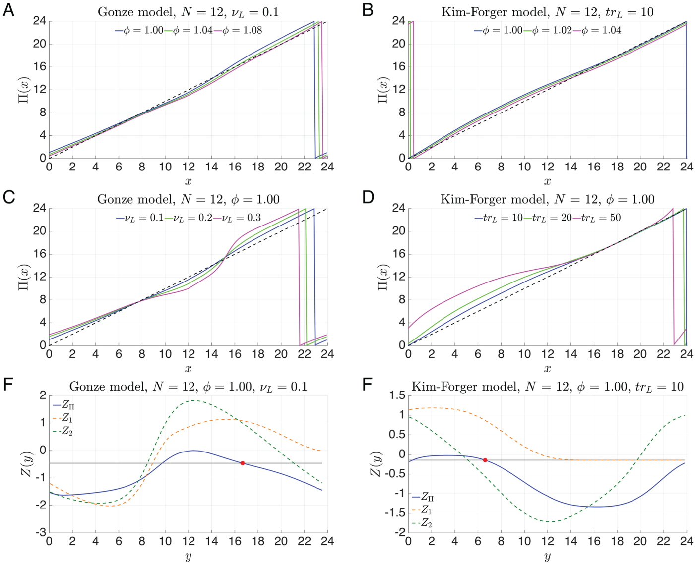
Entrainment maps and PRCs for the Gonze model (left) and Kim-Forger model (right). (A and B) Variations in the maps due to changes in the intrinsic period of the oscillators. As with the NT model Figure 4A, the map shifts down and to the right for faster intrinsic oscillators. (C and D) Stronger light affects entrainment. There is not much difference in the phase of entrainment but a pronounced difference in the concavity of the map, which will lead to faster entrainment. (E and F) Comparisons of the PRC generated from our map, $Z_{\mathrm{\Pi }}(y)$ , versus those generated from perturbations of the DD limit cycle. The red dot is the entrained phase calculated via direct simulation.

In Figures 9C and 9D, we show how the maps behave in response to increases in light intensity ( ${\nu }_L$ in the Gonze model and $t{r}_L$ in the Kim-Forger model). In both models, as light is increased, the phase of entrainment does not change much. Instead, at various places, the concavity of the map increases. As these properties were also found in the NT model (Fig. 6), we would predict that stronger light leads to faster entrainment in both of these models just as it did in the NT model.

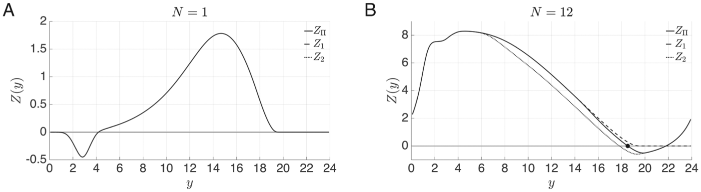
In Figures 9E and 9F, the PRCs $Z_{\mathrm{\Pi }}(y)$ , $Z_1(y)$ , and $Z_2(y)$ are shown for a 12:12 photoperiod. What is interesting about these graphs is how poorly the conventional PRCs Z₁ and Z₂ perform in predicting the entrained phase (red dots). $Z_1$ fails to produce an entrained phase for the Gonze model while producing a set of nonunique solutions for the Kim-Forger model. $Z_2$ is quantitatively incorrect for both models. The reason why the conventional PRC fails is because it is calculated using a perturbation of the DD limit cycle. In contrast, the entrainment map based PRC, $Z_{\mathrm{\Pi }}$ , perturbs off of the LD-entrained solution and produces an accurate prediction. For the Gonze model, it is possible to see that the DD and LD-entrained solutions lie in very different regions of phase space (see Suppl. Fig. S5). So the fact that the PRC and map-based predictions are different is not surprising. For the Kim-Forger model, it is nearly impossible to tell where in phase space the DD and LD-entrained solutions lie. But we would infer that they are not near one another.

Discussion

Circadian rhythms enable organisms to appropriately align physiological and behavioral processes with the 24-h environmental cycles conferred by the earth’s daily rotation. Rhythms persist when the organism is isolated from external time cues; however, in constant conditions the period of circadian oscillators is typically not exactly 24 h. For example, the average human circadian rhythm is 24.2 h while that of mice is 23.5 h (Ripperger et al., 2011). These oscillators are subject to periodic external forcing such as the light-dark cycle that adjusts the phase of the rhythm and entrains them to a period of 24 h. The entrained rhythm must have the proper phasing with respect to external events in order for the circadian system to confer a selective advantage to the organism (Ben-Shlomo and Kyriacou, 2002). Two important questions arise: Under what conditions do circadian oscillators phase-lock to external forcing, and when they do what determines the phase of entrainment?

In this paper, we have developed a new method to determine the phase-locking properties of a circadian oscillator relative to a 24-h light-dark cycle. We derived an entrainment map $\mathrm{\Pi }(x)$ for a 2-dimensional NT model of the Drosophila molecular circadian clock and then showed that the map can be similarly derived for the 3-dimensional Gonze and the 180-dimensional Kim-Forger models of the mammalian molecular circadian clock. In particular, if the oscillator lies on a Poincaré section $\mathcal{P}$ and $x$ is the time from the onset of the most recent light-dark cycle, $\mathrm{\Pi }(x)$ is measured when the oscillator first returns to $\mathcal{P}$ and predicts the time from the beginning of the most recent light-dark cycle. A fixed point of the map corresponds to a phase-locked LD-entrained solution. In all models, for canonical sets of parameters, we showed that the map typically has 2 fixed points, $x_s$ , which is stable, and $x_u$ , which is unstable. Further, since $x=0$ corresponds to where the lights turn on (nominally 0700 h), knowing the value of $x_s$ allows us to determine where along the trajectory in phase space the lights turn on and off. For example, in the NT model with the set of parameters that corresponds to an intrinsic period $\tau =27.6$ (canonical parameter set with $\mathrm{\varphi }=2.2$ ), the LD-entrained solution has the lights turn on 14 h before $M$ reaches its maximum value. This is consistent with biological findings that the highest mRNA levels for Per, an important gene in the Drosophila circadian clock, are found 2 h after lights off in a 12-h:12-h light-dark cycle (Young, 1989).

Using the entrainment map allowed us to understand and predict the effects of parameter changes in the model. Indeed, parameters that have similar effects influence the entrainment map in the same way across all 3 models. For example, increasing $\mathrm{\varphi }$ decreases the intrinsic period of the oscillators. In all cases, the entrainment map $\mathrm{\Pi }(x)$ shifts down and to the right, moving the stable fixed point $x_s$ to smaller values. The analysis also revealed several interesting roles for the unstable fixed point $x_u$ . First, $x_u$ separates the set of initial conditions $x_0$ that entrain via phase advance or phase delay. Second, initial conditions that are in a neighborhood of $x_u$ took the longest to entrain, largely independent of the direction of entrainment. Third, loss of entrainment could occur due to changes in parameters through a stereotypical saddle-node bifurcation when $x_s$ and $x_u$ merge. Some changes in parameters, however, never lead to a loss of entrainment: in particular, increases in light intensity ( $k_L$ in NT, ${\nu }_L$ in Gonze, and $t{r}_L$ in Kim-Forger). Fourth, the existence of $x_u$ implies the existence of an unstable entrained periodic solution. As shown in Figure 3D, this unstable limit cycle is smaller in amplitude than its stable counterpart. It is also shifted by a distance of roughly $|x_s-x_u|$ in terms of when it experiences light relative to the stable limit cycle. For the canonical set of parameters, this implies that when the unstable limit cycle is experiencing light, the stable limit cycle is experiencing dark, and vice versa. Thus, the solutions are effectively 180° out of phase. As $\mathrm{\varphi }$ changes and the system nears a saddle-node bifurcation, the difference in phases between the stable and unstable solutions shrinks (eventually going to 0) and entrainment occurs mostly through phase advance if $x_s>x_u$ or phase delay if $x_s<x_u$ .

The basic idea behind constructing an entrainment map for any particular model is quite general. Namely, in the phase space of the model, choose a Poincaré section along a point of the LD-entrained solution. Then compute the map $\mathrm{\Pi }(x)$ by taking initial conditions that lie at the intersection of the map and the LD-entrained solution and measure the return time to the Poincaré section. $\mathrm{\Pi }(x)$ is then the amount of time that has passed since the onset of lights in the most recent light-dark cycle. As such, the entrainment map will always be 1-dimensional. What will vary is the dimensionality of the Poincaré section $\mathcal{P}$ . As our simulations have shown, even when the Poincaré section is high dimensional, as in the Kim-Forger model, the entrainment map very accurately predicts the stable phase of entrainment. In these high-dimensional cases, the map has the added advantage that effects of changes in parameters are more easily predicted because these changes are stereotypical across models.

Comparison to Prior Work

There are 2 major paradigms for entrainment in the circadian field: discrete (or nonparametric) entrainment and continuous (or parametric) entrainment (Roenneberg et al., 2010a). The former is based on the idea of a free-running oscillator, DD for example, experiencing discrete phase shifts in response to perturbative inputs along its limit cycle and in particular light-dark transitions. This approach has led to methods based on the PRC and does not explicitly take into account the periodic nature of the forcing signal. The second paradigm assumes that entrainment occurs through continuous adjustments to the speed of the oscillator and involves a velocity response curve (VRC) (Beersma et al., 1999; Rand et al., 2004; Taylor et al., 2010, 2014). The VRC characterizes regions in the circadian phase space where the speed of the oscillator increases or decreases as a function of a change of parameter—for example, light intensity. It can be thought of as the variational derivative of the phase with respect to a parameter of interest. This approach is categorized as being continuous, rather than discrete, because it assumes that light affects the oscillator throughout the circadian cycle and not just at light-dark transitions. Both PRC- and VRC-based methods are fundamentally based on using the isochron structure of the underlying DD oscillator to determine the change in phase. The phase of these oscillators is defined relative to a reference point on the DD oscillator itself.

Our approach to studying entrainment is different than these methods in that we view the periodic 24-h light-dark forcing as being the underlying rhythm that sets the reference point for determining phase. Namely we assign the time at which lights turn on as the reference $x=0$ and do not separately define a phase for the DD or LL oscillators. We determine how a circadian oscillator with a prescribed initial condition relative to lights-on adjusts its dynamics over a periodic 24-h light-dark cycle. By considering the 24-h range of possible initial conditions, we obtain the entrainment map $\mathrm{\Pi }(x)$ . Depending on the initial condition, $\mathrm{\Pi }(x)$ is calculated by splitting up either the light or dark pulse over the course of 1 or more 24-h cycles. For example, with 12:12 LD forcing, since $x=0$ corresponds to lights-on, the initial condition $x_0=4$ leads to a computation that starts with the oscillator at $\mathcal{P}$ and imposes 8 h of light, followed by 12 h of dark and then 12 h of light and so on. The value $\mathrm{\Pi }(4)$ is determined when the trajectory first returns to $\mathcal{P}$ independent of whether this time took less than, more than, or the same as 24 h. If, for example, $x_0=19$ , then initially 5 h of dark would be imposed followed by 12 h of light, then 12 h of dark, and so on. In the former case, the light pulse would be split up; in the latter, the dark pulse would be split up. In contrast, PRC- and VRC-based methods only use a single light pulse, and often after imposing too long a dark duration (because they perturb off of DD conditions), which can lead to only a portion of the light pulse being taken into account by the time the oscillator returns to its reference phase.

The entrainment map is similar in spirit to the circadian integrated response characteristic (CIRC), proposed by Roenneberg et al. (2010b), in that both approaches attempt to take into account the periodic nature of the light-dark forcing. Common to all approaches is the need for a well-defined oscillatory solution that can be described as a limit cycle in an appropriate phase space. In most cases, this is the DD limit cycle. The entrainment map, in addition, uses the structure of the LL limit cycle to help define its properties. This is closely related to the suggestion by Peterson (1980), who noted that an LD-entrained solution at some moments in its cycle tries to approach the stable DD cycle and at other moments approaches the LL cycle. Our analysis involving $\mathrm{\Pi }(x)$ does not explicitly incorporate a VRC. However, it does use the fact that changes in parameters differentially affect the speed with which a trajectory evolves in different regions of phase space. For example, we showed how changes to intrinsic parameters $\mathrm{\varphi }$ and $k_f$ of the NT model had a more uniform effect on speed compared with those associated with the intensity $k_L$ and duration $N$ of the light pulse.

These points of difference and commonality aside, the entrainment map is simply a tool to make predictions about the phase-locking properties of a circadian oscillator. As a result, the findings obtained through its use should qualitatively match prior findings that use other methods that themselves match to empirical data. In Bordyugov et al. (2015), the authors derive conditions on entrainment and its dependence on parameters in an abstract setting of the Kuramoto phase oscillator model (Kuramoto, 1984). They then test the predictions made by the phase model on a modified Goodwin model of gene regulation with solely negative feedback (i.e., the Gonze model; Gonze et al., 2005) and on a 19-dimensional molecular clock model (Relogio et al., 2011). They consider a 2-dimensional parameter space consisting of the mismatch between the free-running period of the intrinsic oscillator and the period of the forcing and the relative strength of zeitgeber input to the oscillator amplitude. Their primary finding is that the one-to-one phase-locked solutions form a wedge-like structure (Arnold tongue) in this space and that the range of stable phases that exist within this wedge can span as much as 12 h. In particular, for weak zeitgebers, the 12-h span is achieved over a relatively small span of mismatches in the periods. As relative zeitgeber strength is increased, a larger range of period mismatch is needed to achieve the 12-h span of stable phases. This result is based on some earlier work of Granada and Herzel (Granada et al., 2013) that established the so-called 180° rule, which is another way to say that the range of stable phases spans 12 out of 24 h. Our results are very similar. For example, in Figure 4A, different values of $\mathrm{\varphi }$ correspond to different free-running periods of the DD oscillator. Since we held the forcing period constant at 24, changes in $\mathrm{\varphi }$ correspond to changing the period mismatch, or equivalently to considering a horizontal slice of the Arnold tongue in Figure 1A of Bordyugov et al. (2015). We see from Figure 4A that the range of stable phases spans roughly an 11-h range (x_s≈15.8 when $\mathrm{\varphi }=1.865$ to x_s≈4.8 when $\mathrm{\varphi }=2.506$ ). Using the entrainment map, we could also create a 2-parameter Arnold tongue representation, say for $\mathrm{\varphi }$ and $k_L$ . To do so, we would combine results from Figures 4A and 4C. The Arnold tongue would also be wedged-shaped in the $\mathrm{\varphi }-k_L$ space. For fixed $k_L$ , a horizontal slice is obtained by varying $\mathrm{\varphi }$ between ${\mathrm{\varphi }}_{min}$ and ${\mathrm{\varphi }}_{max}$ , as discussed above. For fixed $\mathrm{\varphi }$ , a vertical slice of the Arnold tongue could be obtained from Figure 4C, which shows that entrainment is lost when $k_L$ decreases (creating a lower edge of the Arnold tongue) but persists as $k_L$ increases.

Granada and Herzel (2009) studied how the time to entrainment is affected by various parameters. One of their main findings, derived for an abstract Poincaré oscillator and then applied to a Goodwin model, is that larger relative zeitgeber strengths leads to faster average entrainment. Their study was specifically designed to minimize the impact of different initial conditions of the oscillators. In our work, we can use the entrainment map to quickly calculate the entrainment time for any initial condition for any fixed set of parameters. Figure 6 shows results for different values of $k_L$ , which is our equivalent to zeitgeber strength. As can be seen from that figure, increases in $k_L$ do result in an average faster entrainment. This can be concluded by visual inspection that the area under the curves decreases as $k_L$ increases. Our work additionally suggests that initial conditions that lie in a neighborhood of the unstable fixed point can take arbitrarily long times to entrain.

From a more mathematical point view, since $\mathrm{\Pi }(x)$ is a circle map, our findings are consistent with the vast literature on forced oscillator models. In the general theory, when a specific parameter is varied, the forced system transitions through a series of different phase-locked (called $m:n$ solutions) and quasi-periodic (often called dense orbits) states. The $m:n$ solutions are actual periodic solutions of the map. These types of solutions occur when the mismatch between the intrinsic oscillator period and the forcing period leads to a rational rotation number, roughly defined as the ratio of oscillator period to forcing period. Dense orbits arise when the rotation number is irrational. These results are a consequence of Denjoy’s theorem on circle maps and subsequent work of Arnold and many others (Arnold, 1965; Glass, 1991; Keener and Glass, 1984). Prior work shows that under certain assumptions, the rotation number varies continuously with a parameter of interest and that there exist parameter intervals over which different $m:n$ solutions can be found. In our case, we focused on one-to-one phase locking, showing that there is an interval $({\mathrm{\varphi }}_{min}\mathrm{,}{\mathrm{\varphi }}_{max})$ for stable entrainment. We did not exhaustively explore the existence of dense orbits or other solutions with rational rotation numbers, but we expect those to exist. Circle maps are also widely used in other contexts such as cardiac dynamics and, more generally, any process that involves clocking (Winfree, 2001). In such cases, a phase transition curve (PTC) is used to build a map to predict the effect of periodic forcing. The PTC measures the normalized phase of resetting as a function of the normalized stimulus phase. By normalized we mean that phase values lie between 0 and 1. The associated map at each cycle then measures the new phase as a function of the old. The PTC, therefore, is constructed using the PRC. Thus, PTCs face the same limitations in their use that PRCs do and can make predictions that are not borne out by a direct simulation or experiment; see Glass et al. (2002).

Future Directions

In this paper we have focused on light-dark forcing since it is the dominant zeitgeber for circadian clocks. However, the entrainment map can readily be extended to nonphotic entraining signals, such as temperature cycles, and perhaps give insight into how the circadian system integrates information from multiple environmental signals occurring simultaneously. The ease with which time to reentrainment can be calculated and visualized for different initial conditions by cobwebbing makes the map a useful tool for investigating jetlag scenarios. The map may also prove to be an effective tool for studying entrainment and synchronization in networks of coupled oscillators.

Entrainment maps of detailed molecular clock models such as Kim-Forger can be used to generate hypotheses about how specific mutations or other manipulations of clock components affect entrainment and to make predictions regarding entrainment mechanisms that can then be tested experimentally. One interesting question to explore using entrainment maps is the effect that different proposed mechanisms of transcriptional regulation (such as protein sequestration and Hill-type repression) have on entrainment properties (Kim et al., 2014; Kim, 2016).

Beyond circadian oscillator models, we believe that entrainment maps can also be successfully constructed based on data from real organisms or experimental preparations. To illustrate our suggested protocol, we consider the cyanobacterial circadian clock, for which the phosphorylation status of the protein KaiC is a convenient phase marker both in vivo and in vitro (Kim et al., 2015). To construct phase response curves for in vivo cultures, experimentalists maintain the cultures in constant light and then expose them to 4-h dark pulses at different phases and measure the resulting phase shift (Kim et al., 2012). To construct an entrainment map, we would instead maintain the cultures under a 12:12 LD cycle. The minimum of the KaiC phosphorylation waveform will play a role analogous to the Poincaré section $\mathcal{P}$ . Once the culture is entrained, there will be a stable phase relationship between the onset of lights and the minimum of the KaiC phosphorylation rhythm. This gives us one data point for the map, namely the stable fixed point $x=\mathrm{\Pi }(x)$ . To obtain other data points, we will measure how the entrained oscillator responds to phase shifts in the LD cycle. Specifically, in one cycle we will extend the light or dark duration by a certain number of hours and then record the time of 2 subsequent minima of the KaiC phosphorylation waveform. This will give us an ordered pair $(x\mathrm{,}\mathrm{\Pi }(x))$ . In fact, each KaiC phosphorylation minimum observed until the culture reentrains will give us one additional data point for the map. Once the culture has reentrained, we can repeat the experiment with a different phase shift of the LD cycle to sample other areas of the map. Alternatively, the experiment can be done in parallel rather than serially by dividing the cyanobacterial culture into a population of subcultures and applying different LD phase shifts to each subculture.