Solar variability imprints on palaeoclimatic records from northwestern Himalaya

Abstract

Understanding the impact of the Sun on climatic variability is crucial when analysing the current state of global warming and climate change. The present study is an initiative to elucidate the low-frequency (interannual and more extended period) variability in two paleoclimatic records obtained from Himalayan cedar and neoza pine tree rings from Lahaul, Himachal Pradesh, and Kishtwar, Jammu & Kashmir, for the time intervals of 1460–2008 CE and 1383–2017 CE, respectively. Time-series analysis was performed to re-examine the tree-ring chronologies using the wavelet transform. The strong interannual variability of a 2- to 4-year timescale was present throughout the record. There was a notable decadal fluctuation, which is ascribed to the well-known 11-year solar cycle. Long-term variability of nearly 30–35 years and 60 years was also present during specific time scales. The wavelet coherence between tree-ring chronologies and sunspot numbers was also investigated to assess time-varying correlations. The present investigation provides evidence of solar activity effects/modulation on tree-ring growth in the northwestern Indian Himalayan region. The results are in good agreement with studies based on tree-ring chronologies conducted in other regions of the world. This suggests a strong control of solar variability on climate in the western Himalaya, particularly with respect to precipitation, by the westerlies as well as the Indian summer monsoon.

INTRODUCTION

The Sun-Earth system gives increasing evidence that climate dynamics are influenced by a variety of factors (Bard & Frank, 2006; Crowley, 2000). Variability in solar radiation is an important external climatic forcing element for Earth (Beer et al., 2006). Understanding the impact of solar forcing on climate change and global warming is critical when studying the Sun’s role in contemporary climate variability (Hoyt et al., 1997; Usoskin, 2017). Instrumental records cover only a tiny portion of Earth’s history, spanning nearly a century. Reconstructing ancient climates is important for understanding natural variability and the development of the present climate. Paleoclimatic proxy records provide a longer-term perspective on climate change than observational weather records, allowing us to investigate prevailing patterns of climate variability over time. One of the most valuable proxy records of past climate changes preserved naturally is tree rings (Groenendijk et al., 2025).

In the world’s temperate and boreal forests, trees grow a new layer of wood around their trunks every year. These rings, which are among the most visible markers of the passage of time in nature, also provide information about the tree’s immediate environment, such as temperature fluctuations, precipitation levels, and other environmental conditions, via their growth patterns. During the ‘Common Era’ (CE, the last two millennia), tree growth rings served as the predominant source of past climatic data. In recent decades, the Intergovernmental Panel on Climate Change has prominently focused on CE in its reports and policy summaries (Esper et al., 2024). For this time frame, annually resolved tree-ring chronologies, used as a climate proxy, are considered one of the most reliable sources of climate data (Cook & Kairiukstis, 2013; PAGES 2k Consortium, 2017).

Moreover, the utilisation of advanced mathematical and computational techniques has significantly enhanced data comprehension. To understand the spatio-temporal variation of time series, wavelet time-frequency analysis is employed by various authors worldwide in tree-ring chronologies (Addou et al., 2023; Grinsted et al., 2004; Halberg et al., 2010; Jia & Liu, 2019; Kasatkina et al., 2019; Land et al., 2020; Rigozo et al., 2002, 2007; Sen & Kern, 2016; Torrence & Compo, 1998). The current study examines published records of tree rings from Himalayan cedar and neozao pine in Lahaul, Himachal Pradesh, and Kishtwar, Jammu & Kashmir, India. To investigate the temporal variability of climate in the western Himalayan region, the wavelet transform and wavelet coherence are employed as computational tools (Li et al., 2019; Nordemann et al., 2001; Singh et al., 2021; Yadav & Bhutiyani, 2013).

METHODOLOGY

Study site and data source

In the present investigation, two distinct climate reconstruction time series from the western Himalaya in India were selected. Annually resolved tree-ring chronologies are invaluable for palaeoclimatological studies. These records were chosen for their geographical range, climate signal, tree species’ foliage, record length, and resolution. These reconstruction records are made available to the public on the National Centres for Environmental Information’s National Oceanic and Atmospheric Administration website (https://www.ncdc.noaa.gov). Additional details on the chronology and analysis procedure for the tree-ring data are given in the original articles (Singh et al., 2021; Yadav & Bhutiyani, 2013). The present analysis uses tree-ring chronologies from Lahaul, Himachal Pradesh, India (TS1, Figure 1), and Kishtwar, Jammu and Kashmir (TS2, Figure 1), previously collected and published by other authors. No new field sampling was conducted for this investigation; all tree-ring material and chronology data were obtained from the sources mentioned. Additionally, data comprehension has been enhanced by contemporary mathematical and computational methodologies. Sunspot number data from the past 250 years has been used to compare solar variability (https://www.ngdc.noaa.gov/stp/solar/).

Figure 1.

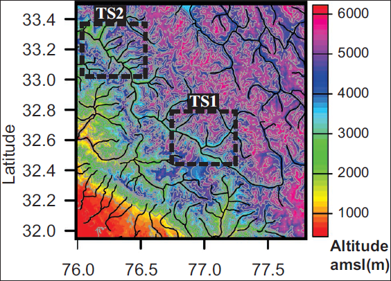
Elevation contour map of the sampling site, with contours delineating varying elevations; river bodies and their tributaries are depicted in black. The vertical coloured sidebar indicates altitude above mean sea level (amsl) in metres. Here, TS1 and TS2 indicate the time series first and second, respectively.

Wavelet analysis

Wavelet analysis examines multiscale signals that are localised in both frequency and time. It is especially beneficial for examining quasiperiodic and intermittent variations. In this study, we utilised the Continuous Wavelet Transformation (CWT) to analyse the time series of tree-ring chronologies. CWT provides localised spectral information regarding the investigated dataset. Similar to a zoom lens, it utilises a variable-size window that constricts when focusing on small-scale/high-frequency signal characteristics and expands when focusing on large-scale/low-frequency signal characteristics. The primary benefit of CWT is its ability to identify prevailing periodicities and specify the time intervals throughout which they may persist.

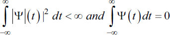
This approach is exemplary for analysing multiscale, nonstationary systems within finite spatial and temporal domains. The wavelet domain visualisation enhances the signal’s dimensionality by integrating energy across both time and scale (or frequency) axes, producing three-dimensional outlines. A one-dimensional time series is converted into a two-dimensional graphic that illustrates the time-dependent evolution of scales and frequencies following the transformation. A wavelet is a diminutive wave that is temporally localised. It is crucial that the wavelet function ψ(t) complies with the requirements of having finite energy and zero mean, namely,

$$\underset{-\infty }{\overset{\infty }{{\displaystyle \int }}}\left|\Psi \right|\left(t\right){|}^{2 }dt <\infty and \underset{-\infty }{\overset{\infty }{{\displaystyle \int }}}\Psi \left(t\right) dt=0$$

CWT is the convolution (or inner product) of a discrete sequence (time series) x_n with a collection of ‘wavelet daughters’ generated by translating and scaling the ‘mother wavelet’. The following statement expresses the convolution:

$${\displaystyle \sum }_{n^{\prime }=1}^n\left(\frac{\delta t}{s}\right)x_{n^{\prime }}{\Psi }^{*}\left[\frac{\left(n^{\prime }-n\right)\delta t}{s}\right], n=1,2,3,. . . . N$$

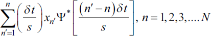
where, analysing wavelet Ψ(t) is referred to as ‘mother wavelet’, whereas Ψ* is its complex conjugate. The scale parameter is presented by s, time index by n, and the sample interval by t. Dilatation (s > 1) and contraction (s < 1) of the wavelet are regulated by the scale parameter.

In this investigation, we take into account the Morlet wavelet as the mother wavelet. The Morlet wavelet can be characterised as a plane wave that is modulated by a Gaussian, as represented as follows:

$$\Psi \left(t\right)= {\pi }^{\frac{-1}{4}} e^{i{\omega }_{0}t} e^{-\frac{t^2}{2}}$$

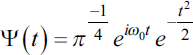
Dimensionless frequency (order of mother wavelet) ω_ο = ₂ύf_ο; f_ο is the central frequency; t is dimensionless time.

In addition, wavelet analysis can be utilised in order to investigate the connection that exists between two-time series. Wavelet Coherence is a bivariate framework for investigating time-series correlations and evolution in continuous time and frequency space. The wavelet coherency portrays the co-movement of two series over time, thus closely reflects the behaviour of a typical correlation coefficient in the time-frequency (or time-period) plane. Since it can show how the time series compares in phase, locally phase-locked behaviour can be identified. Wavelet coherence can establish significant coherence even with low CWT common power.

The mathematical efficiency of wavelets can be transformed into practical utility through the application of advanced computational techniques. In this instance, the CWT was computed using Wavelet Comp, an open-source software package developed in R (Torrence & Compo, 1998). In the WaveletComp software package, wavelet theory and applications are viewed as an extension of statistical methods ‘R’ (R Core Team, 2018).

RESULTS AND DISCUSSION

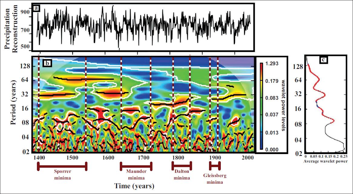
The wavelet spectrum of the tree-ring chronology data from the northwestern Himalaya is shown in Figures 2a and 3. Figure 2a depicts a time series obtained from the tree-ring (TS1) chronology. Figure 2b presents the wavelet power spectrum, where the horizontal axis denotes the time dimension, the vertical axis denotes the period, and power is shown in varying colours. White contour lines denote the 95% confidence level, while black lines signify the ridges. The area above the ∩-shaped curve signifies the cone of influence (COI). The black lines indicate the ridges of the component overlay on the CWT image. The vertical dashed lines indicate the Spörer, Maunder, Dalton, and Gleissberg minima, respectively. The vertical bar on the right side of the CWT spectra indicates the colour code for spectral amplitude, with blue representing low power and red representing high power. Figure 2c illustrates the average wavelet power of the series. Figure 3a illustrates the time series derived from tree-ring chronology. Figure 3b presents the wavelet spectrum, while Figure 3c displays the average wavelet power for the same series.

Figure 2.

(a) A time series derived from tree-ring (TS1) chronology in the NW Himalaya, (b) illustrates the wavelet power spectrum, with the horizontal axis representing the time dimension, the vertical axis indicating the period, and power represented by different colours. White contour lines indicate the 95% confidence level, while black lines represent the ridges. The area above the ∩-shaped curve signifies the cone of influence (COI). Additionally, the ridges of the component superimposed over the CWT image are represented by the black lines. Further, the vertical dashed lines delineate the Spörer, Maunder, Dalton, and Gleissberg minima, respectively. The vertical bar on the right side of the CWT spectra represents the colour code for spectral amplitude, ranging from blue (indicating low power) to red (indicating high power), and (c) the average wavelet power of the series.

Figure 3.

The figure description is the same as Figure 2, but for TS2.

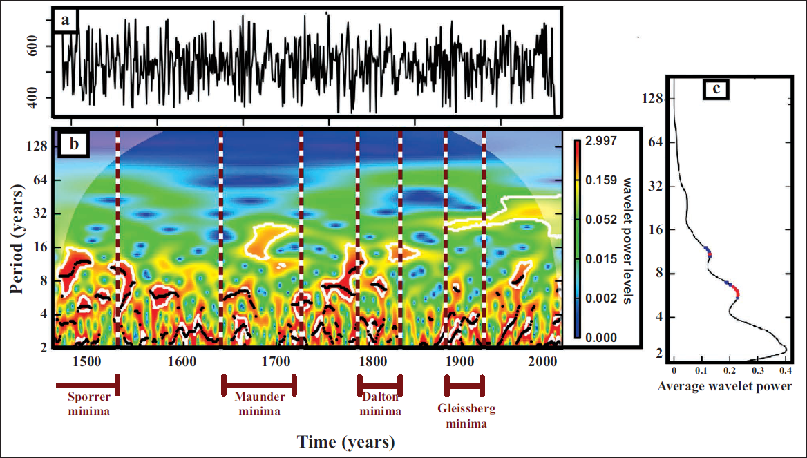
Figures 2 and 3 indicate significant interannual-to-multi-decadal-scale variability in regional climate between the analysed time series, namely, 1384–2017 CE and 1400–2000 CE. The strongest periodicity is evident in the 2–4-year band in both the time series and ubiquitously present throughout the records, indicating extreme interannual variability of precipitation in the western Himalaya (Figures 2b–3b). Another sub-decadal-scale variability occurred in the 4–8-year band, appearing intermittently across all time intervals, though weaker than that of the 2–4-year band (Figures 2b–3b). The 4- to 8-year cyclicity is not clearly visible in the period between the Dalton minimum and the Gleissberg minimum (1830–1890 CE). In comparison to TS1, 4–8-year periodicity was stronger in TS2.

The third most prominent periodicity lies in the 7–15-year band, centred at ~11 years and covering most of the time series. The 11-year periodicity signal is uniformly strong and pronounced throughout the time series, stronger in TS1, especially during solar minima, and suppressed during warmer intervals. The ~11-year cyclicity is less pronounced after 1870 (Figures 2–3). The variability of the 19–25-year band can also be observed between 1550 and 1800 CE. The 19–25-year periodicity is more pronounced in intervals where the 7- to 15-year band variability is suppressed or reduced (Figure 2). An intriguing cyclicity of around 30–35 years is evident between 1400 and the beginning of the Maunder Minimum, which reappears after 1900 CE, with a cessation of around 300 years.

In addition to the low-frequency (short-period) variation in precipitation time series, WPS exhibits high variability in long-period variations on decadal timescales. A periodicity of approximately 10–11 years appears to be distributed throughout the time series signal. Different time frames, such as (1500–1600), (1650–1700), and (1820–1880), each exhibited periodicity of 15–16 years. During (1350–1500), (1550–1650), and (1750–1840), there was variation in the 30-32-year period (1900–2000). Also observed throughout this period (1440–1620) was a 64-year span.

Additionally, a long-term periodicity of ~60–80 years was evident throughout the record, except for the interval between the Maunder Minimum and the Dalton Minimum. Another long-term variability existed in a 130–140-year band throughout the record, but it was not very prominent.

Wavelet Coherence

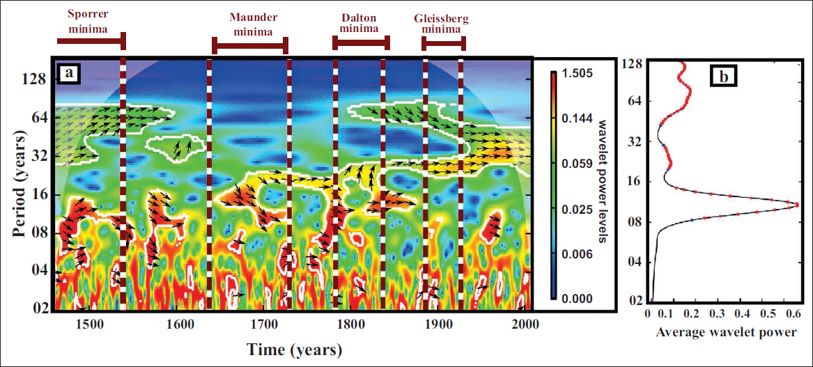
To understand the time-varying relationship between the tree-ring and reconstructed climate variability in the western Himalaya, we used wavelet coherence. The WTC reveals notable coherence and a positive correlation between the two time series at sub-decadal to decadal time scales (Figure 4). Both time series observed in-phase coherence for the 7–15-year band, centred at around 11 years, are evident throughout the record (Figure 4). Other strong periodicities in 2–4 year and 4–8 year bands also clearly show an in-phase coherence. A strong coherence of 25–35 appeared at around 1700 CE and persisted until 2012 CE. Another multi-decadal synchronicity of 60–80 years spanned 1440 and 1580 CE, but it diminished thereafter; however, the relationship is not strong.

Figure 4.

Wavelet coherence between TS1 and TS2. The horizontal axis denotes the temporal dimension, while the vertical axis illustrates the period, with power shown by multiple shades of colour. White contour lines indicate the 95% confidence level. An arrow directed left signifies anti-phase, indicating that the two time series exhibit negative correlation, whereas an arrow directed right denotes positive correlation between the two time series. An upward arrow suggests the second time series leads the first, while a downward arrow means the first leads the second. Further, the vertical dashed lines delineate the Spörer, Maunder, Dalton, and Gleissberg minima, respectively. (b) represents the average wavelet power.

The CWT and wavelet coherence of the tree-ring record from the northwestern Himalaya illustrate significant variability at sub-decadal to multi-decadal scales. They are strongly influenced by solar activity in modulating the regional climate. The 2–4-year band represents the interannual variability of the precipitation in the western Himalayas. Similar conditions and periodicities are evident throughout the Indian subcontinent, and the occurrence of the same precipitation in two consecutive years is very unlikely in the region (Gupta et al., 2019).

The periodicity of the 4–8-year band corresponds to the second harmonic (5.5 years) of the Schwabe cycle, and it is persistent in the wavelet spectra of all heliogeophysical records. A very strong 11-year periodicity demonstrates the influence of solar cycle variability on precipitation and, in turn, on tree-ring growth in the western Himalaya. The effects of the sunspot cycle (11 years, Schwabe cycle) and the double sunspot cycle (22 years, Hale cycle) on climate variability are evident worldwide, as evidenced by these periodicities in high-resolution paleoclimatic records. For annual precipitation amounts over Central Europe, similar power peaks were identified in spectral analyses with durations of 2–4 years and 10–16 years. Furthermore, the significant power peaks identified in an additional hydroclimate record derived from tree rings at approximately 15, 7.5, 5.8, and 2.7 years from the northern boundary of the current research region exhibit a high degree of agreement (Dutt et al., 2019, 2021; Gupta et al., 2019, 2021).

Our results reinforce these previous findings. CWT results of the sunspot number (SSN), total solar insolation (TSI), and corresponding wavelet coherence are shown in the supplementary file (S-Figures S1–S3). They also indicate a powerful influence of the 11-year periodicity on TSI between 1600 and 2012 CE, implying the significance of the 11-year Schwabe cycle in controlling low-frequency climate variability on Earth. Similar periodicities are also observed in available low-frequency proxy reconstructed climate records for the Indian summer monsoon, Rewalsar Lake, western Himalaya (Singh et al., 2020), and Wah Shikar and Mawmluh Cave from northeast India (Dutt et al., 2021; Gupta et al., 2019), and East Asian summer monsoon records from the Hulu and Dongge caves from China (Cheng et al., 2001; Wang et al., 2005). Likewise, the periodicity of 16–25 years reflects the double sunspot cyclicity, which is also evident in several regional reconstructions of past climate variability (Cheng et al., 2001; Dutt et al., 2018). The 17–18-year cycle is sometimes referred to as the Brückner cycle and is attributed to the lunar effect on Earth’s climate. The wavelet decomposition, however, revealed that these periodicities are not stable and linear throughout the past centuries. The Schwabe cycle is absent during the Maunder Minimum. The MM was the period of very low or no sunspot activity (Eddy, 1976). Further significant volcanic eruptions occurred during the MM, and large amounts of volcanogenic sulfur, other gases, and ash were dispersed into the atmosphere (Miller et al., 2012). This may be the reason for the non-observable effect of 11 years of solar variability on tree-ring growth and precipitation in the western Himalaya.

The 30–40-year cyclicity is also possibly related to solar variability. The CWT of TS1 exhibits similar patterns over the past four centuries. A multiproxy record from Tso Moriri Lake in the western Himalaya has evidenced 33- and 37-year periodicity over the last 4500 years, suggesting it as a prominent modulator of multi-decadal variability in the regional climate of the NW Himalaya (Dutt et al., 2018). A 35-year climate cycle is also evident in several tree-ring records from Europe and the Arctic regions. The multi-decadal oscillations in the North Atlantic Ocean are also responsible for the 35-year periodicity. Meteorological and monitoring data show that the mid-latitude westerlies receive the majority of the precipitation in the study region during winter. These westerlies have a strong influence on the North Atlantic and Arctic climate and, therefore, might have transmitted the signal of the North Atlantic Oscillation to tree-ring growth and precipitation in these parts of the western Himalaya. In our view, the cyclicity of around 30–35 years in the tree-ring records from the western Himalaya primarily reflects the combined effects of the 35-year cyclicity of solar insolation and North Atlantic Oscillations. Solar insolation is a primary factor that also influences the North Atlantic Oscillation.

The other periodicities of the 65–85-year and 130–140-year bands are also the possible manifestations of the Gleissberg solar cycle (77 years) and the half-de Vries cycle (210–220 years). Broadly, changes in solar insolation and the North Atlantic Oscillation principally modulate the low-frequency climate variability, occurring on a sub-decadal to multi-decadal scale, in the westerlies that dominate the higher reaches of the western Himalaya. Higher solar insolation results in a higher pressure gradient between the Indian Ocean and the Indian subcontinent due to differential heating of the ocean and landmass, thereby strengthening the ISM. Stronger ISM conditions push their limits further north in the Himalaya and shift the mid-latitude westerlies into Central Asia and further north to the Himalaya. Stronger ISM conditions are aligned with weaker westerlies influence in the NW Himalaya. Higher insolation further elevates the temperature of the atmosphere, the North Atlantic, and the Arctic regions and weakens the westerlies-mediated precipitation in the NW Himalaya and vice versa.

The continuous wavelet transform shows high power in the ∼60-year frequency domain until ∼1500 CE, but appears highly significant only in the second half of the eighteenth century. To investigate the time-varying correlation between tree-ring data and sunspot numbers, wavelet coherence analysis was performed. Wavelet coherence pattern (WCP) is basically used to illustrate the relationship between two time series (Figure 4). Wavelet coherence plots emphasise co-moving areas in time-frequency space. The warmer the colour, the higher the coherence (or correlation) in time-frequency space, from dark blue (0, no coherence) to red (1, strong coherence). In Figure 4, the black arrows depict the phase of the wavelet and the direction of movement for the two series. Statistically significant coherence is outlined in black. The direction of the aligned arrows indicates both the correlation and the time series that is driving the relationship at that instant. Left-pointing arrows indicate negative correlations between time series. Right-pointing arrows indicate good correlations between time series. An arrow pointing down means that the first time series comes before the second, while an arrow pointing up means the opposite.

The available datasets on sunspot cycles, spanning the years 1700–2017, were used for the analysis. The time series of sunspot number, along with its wavelet spectrum, is depicted in the supplementary file (Figures S1–S3, respectively). WCP between precipitation and sunspot number exhibits several regions of strong coherence, as depicted in. WCP between the two time series over the last three centuries (1700–2017) revealed a strong correlation in the 9–12-year periodic band. Within this band, the two-time series appear nearly in phase over the studied timescale. Another coherence pattern during 1950–2000 in the 30–34-year periodic band was also visible. Relatively weak coherence was observed in the 60–65-year periodic band during approximately 1750–2000. The periodic cycles were compared with the sunspot numbers (supplementary file). This builds on records based on direct, visual, solar observations of sunspots on the Sun, which are available only for the last 400 years. Successions of longer-lasting grand solar minima and solar maxima clearly stand out in our reconstruction and were (re-)defined with respect to both magnitude and timing. The high similarity between the two radionuclides 14C and 10Be, as well as the fact that well-known grand solar minima, such as the Maunder and Dalton minima, are well represented in radionuclide records, confirms that these records primarily reflect production changes driven by variations in cosmic-ray fluxes. The solar maximum between the Spörer and Maunder minima (AD 1558–1621) is noticeably weaker. The Sun appears not to have fully recovered during the period corresponding to the Little Ice Age (AD 1400–1850). The current analysis shows a consistent and significant reduction in solar modulation during this period. Limited studies based on wavelet analysis of tree-ring chronologies have been done from the western Himalayan region (Malik & Sukumar, 2021; Panigrahi et al., 2006).

The comparison of the time series of solar activity and its wavelet spectrum (Supplementary figures) indicates that grand solar minima tend to coincide with the minima of the de Vries cycles (it is important to note that solar activity is represented on a reversed scale in). The comparison of solar activity and climate time series alongside their wavelet coherence indicates that, generally, during the Hallstatt cycle, periods of reduced solar activity—marked by significant de Vries cycle amplitudes and frequent grand solar minima—correlate with a weaker AM. There exists a discrepancy during the Hallstatt cycle minima between 5,000 and 6,000 BP, as well as in the past 1,500 years. The wavelet coherence for the periodicity of the de Vries cycle (approximately 210 years) is low during these periods, despite the visibility of several grand solar minima. Temporal differences are expected because the Sun is not the sole driver of the climate system; other forcing factors, including volcanic aerosols and greenhouse gases, have varied over time, thereby obscuring the solar fingerprint.

CONCLUSIONS

This study represents a time-series reanalysis of tree-ring chronologies from the northwestern Himalayan region of India using advanced mathematical and computational tools. The chronologies demonstrate the strong solar influence. Interannual periodicities of 2–4 years were prominent. It was consistently observed that the prominent 11-year solar cycle falls within the 7- to 15-year range. A prominent 30- to 35-year cycle is observable from 1400 onward until the commencement of the Maunder Minimum. The record also indicated a long-term periodicity of 60–80 years, except during the Maunder Minimum and Dalton Minimum. Wavelet coherence demonstrates that both time series exhibit phase coherence within the 7–15-year band, centred at 11 years, throughout the entire record.

The current study demonstrates the effectiveness of applying sophisticated mathematical and computational methods to paleoclimatic time series, and it will be expanded in the future to extract valuable information from the wealth of paleoclimatic time series.