Sage Journals: Discover world-class research

Abstract

Reduction of wasting, or low weight-for-height, is a critical target for the Zero Hunger Sustainable Development Goal, yet robust evidence establishing continuous seasonal patterns of wasting is presently lacking. The current consensus of greatest hunger during the preharvest period is based on survey designs and analytical methods, which discretize time frame into preharvest/postharvest, dry/wet, or lean/plenty seasons. We present a spatiotemporally nuanced study of acute malnutrition seasonality in African drylands using a 15-year data set of Standardized Monitoring and Assessment of Relief and Transition surveys (n = 412,370). Climatological similarity was ensured by selecting subnational survey regions with 1 rainy season and by spatially matching each survey to aridity and livelihood zones. Harmonic logit regression models indicate 2 peaks of wasting during the calendar year. Greatest wasting prevalence is estimated in April to May, coincident with the primary peak of temperature. A secondary peak of wasting is observed in August to October, coinciding with the primary peak of rainfall and secondary peak of temperature. This pattern is retained across aridity and livelihood zones and is sensitive to temperature, precipitation, and vegetation. Improved subnational estimation of acute malnutrition seasonality can thus assist decision makers and practitioners in data-sparse settings and facilitate global progress toward Zero Hunger.

Plain language title

Fifteen Years of Rapid Assessment Surveys Indicate Seasonal Variability in Prevalence of Acute Malnutrition Among Children Younger Than 5 Years in African Drylands

Plain language summary

Wasting or low weight-for-height is a key indicator of short-term or acute malnutrition. The timing of highest wasting prevalence, particularly among children younger than 5 years, is of interest for humanitarian efforts to reduce hunger. Current knowledge about this timing derives from survey designs, which discretize continuous time into preharvest/postharvest, dry/wet, or lean/plenty seasons. Instead of this categorical approach, we utilize harmonic regressions that allow for modeling of continuous time in our analysis of 15 years of Standardized Monitoring and Assessment of Relief and Transition surveys. Surveys conducted in parts of North Africa with 1 rainy season (unimodal regions) were selected for similar climate, and survey locations were further subdivided by aridity and livelihood zones. The seasonal pattern of extreme wasting prevalence in each group was modeled using survey data for a total of 412,370 children. We identified 2 periods of highest wasting prevalence in April to May and August to October. The April to May peak occurs during highest temperatures, and the August to October peak occurs during periods of highest rainfall and warmer temperatures in the study area. These findings can inform the timing of nutrition programs in unimodal dryland regions and guide future quantitative models of acute malnutrition seasonality.

Keywords

acute malnutrition wasting seasonality drylands SMART time series analysis

Introduction

The Zero Hunger Sustainable Development Goal (SDG 2) aims to end all forms of malnutrition by 2030.¹ This includes the achievement of global targets on wasting, defined as weight-for-height z-score less than 2 standard deviations below the established median.^1,2 In 2019, approximately 47 million children younger than 5 years were affected by wasting, representing a global public health priority.^3,4 However, monitoring of wasting trends over time is particularly challenging since wasting is highly seasonal.^5,6 Global prevalence estimates of wasting are based on infrequent national household surveys conducted every 3 to 5 years and often during the same seasons.^3,7 Prevalence calculated from such surveys are point estimates that are not representative of wasting during a calendar year, across multiple years, or even across administrative boundaries due to staggered survey timings.⁷ These methodological limitations are evident in the lack of trend data for wasting compared to child stunting and overweight in key publications addressing acute malnutrition.^3,4 In the absence of high-resolution survey data for effective measurement, the seasonality of wasting remains a critical “missing piece” of knowledge, which limits our ability to measure progress toward SDG 2.^3,7

Current understanding of wasting seasonality is also limited by widely held assumptions, existing analytical methods, and available primary data. Nutrition studies are routinely designed or analyzed at one point in time, frequently scheduled to occur at the same time each year as a way to control for seasonality, timed to coincide with assumed peaks in malnutrition, or designed using discrete categories such as preharvest versus postharvest, dry versus wet season, or hunger/lean versus plenty season. This categorical breakdown is far less nuanced compared with local seasonal calendars, which may reflect as many as 5 or 6 distinct seasons.⁸ We posit that this temporal aggregation of seasons into categories derives in part from a deeply engrained “food-first” bias among policy makers and in emergency programing, which assumed that malnutrition was driven primarily by a lack of food.⁹ This assumption has arisen in part from extensive research on agrarian decisions in alignment with meteorological factors, thereby linking seasonal experiences of hunger to agrarian seasons.^10
-12 The preharvest period was identified as the period of “overlapping and interacting” vulnerabilities¹⁰ and, therefore, the period of greatest hunger. Although the “food-first” assumption has been overturned in favor of multicausal pathways to acute malnutrition in recent decades,^9,13 the assumption that the preharvest period is the “hungry season” is widely held and frequently used to justify the timing of food aid and nutrition interventions. Recent studies indicate more variability in the timing of greatest acute malnutrition and emphasize differences across climatic zones.^5,8,14

-17

Assumptions around peak timing of acute malnutrition also directly relate to the dominant livelihood production system, such as pastoralism or farming. Peak timing for pastoralism is generally assumed to be at the end of the dry season when pasture is limited and fewer animals are at the homestead, resulting in less availability of animal milk for children.¹⁸ On the other hand, peak timing for households, primarily practicing cultivation, is generally assumed to occur prior to the harvest season related to crop availability and pricing.¹⁹ However, there is limited literature that directly compares different livelihood systems in relation to acute malnutrition seasonality. One exception is Bechir et al (2010), who find that the prevalence of acute malnutrition in Chad is higher for both pastoralists and farmers before the rainy season as compared to after—indicating comparable seasonal patterns across the 2 livelihoods.²⁰ Chotard et al (2010) also compare across livelihood groups in the Greater Horn of Arica but only identify that there is greater seasonal fluctuations among pastoralists.⁵ Both studies utilize categorical variables of rainy/dry and hunger/moderate/postharvest seasons for the temporal domain.

The pervasive hungry season assumption has influenced data collection instruments including national surveys, which provide input data for SDG target monitoring. However, the lack of frequent and concurrent observations in these surveys limits any analysis of wasting seasonality or trends over time. National surveys also utilize administrative boundaries for sampling designs, thereby combining observations across different climatological and agroecological zones despite known spatial variability in environmental phenomena and nutrition. In addition to temporal biases in data collection, analytical methods for survey data are structured as seasonal comparisons of wasting against a reference postharvest period when wasting is assumed to be low from similarly aggregated studies.¹¹ Temporal aggregation from day and month to seasons in such analyses, therefore, yields an incomplete understanding of fluctuations during the calendar year. Thus, our knowledge of wasting seasonality remains limited in both space and time due to the lack of agroecologically comparable primary data and due to temporal aggregation as the established methodology for seasonality analysis, respectively.

The lack of high-frequency and high-resolution data on nutrition status can be addressed with secondary data, such as pooled nutrition surveys. These data provide a long-term record of frequent cross-sectional observations in multiple locations to effectively analyze seasonality. Secondary data also provide an opportunity to study nutrition outcomes alongside covariate factors such as livelihoods, climate, and conflict. One valuable secondary data set to study nutrition seasonality is the 15-year compilation of child-level anthropometry from Standardized Monitoring and Assessment of Relief and Transition (SMART) surveys.²¹ The SMART survey methodology utilizes standardized survey questionnaires to measure nutritional status of children younger than 5 years.²² The SMART surveys also utilize a reliable cluster sample size of at least 900 children from 30 households in 30 clusters.²² The comparable survey methodology over time allows for reasonable time series analysis of data from SMART surveys. The compiled SMART data set has previously been used to study the relationship between stunting and wasting in emergency contexts.²¹ Although this data set is biased toward rural populations facing complex crises,⁸ it provides precious data on extreme wasting in critical populations. The pooled SMART data set can be augmented to improve analysis of seasonal malnutrition through spatial and temporal disaggregation of survey variables. Access to the month and year of SMART survey implementation enables continuous time series analysis of seasonal patterns, and access to the administrative region of survey implementation allows for spatial alignment with critical variables such as livelihood and climatic zones. Thus, the cross-sectional SMART survey data set can inform key nutrition interventions and humanitarian actions to more effectively reduce seasonal wasting.

The methodological limitation of temporal aggregation can also be addressed with harmonic regression, which utilizes continuous temporal variables for seasonality analysis. Harmonic regression is widely applied in epidemiology to estimate the seasonal disease burden and outbreak trajectory of infectious diseases and foodborne illnesses.^23
-25 Due to its simple use of sine and cosine functions to decompose the dependent variable, harmonic regression is particularly useful for modeling cyclical processes such as precipitation or disease without discretizing temporal variables.^24,26,27 Harmonic regression also provides an intuitive method for estimating peak timing and maximum expected value based on estimated harmonic coefficients. Peak timing estimation is frequently utilized to predict the time of highest incidence of a disease^28

-31 and can be extended to estimate the time period and estimated prevalence of greatest wasting. At the time of writing, the authors are aware of only 3 nutrition seasonality studies that utilize harmonic regression analysis.^15,32,33

We present a nuanced study of wasting seasonality in the African drylands using the combined 15-year SMART survey data set. First, we demonstrate the application of harmonic regression with the first and second harmonics to nutrition data. Previous studies on this topic only model first harmonics (2π), thereby identifying only one period of acute malnutrition during the calendar year.^15,32,33 Inclusion of second harmonic terms (4π) is required to allow for the possibility of a second peak in the calendar year where statistically significant.^26,27,34 Remaining studies and routine national surveys rely on 1 to 3 observations during a calendar year, which are insufficient to establish the month-to-month pattern of wasting. Correct application of harmonic regression can provide a reliable and adaptable model, which can identify 1 or more periods of high wasting.

Second, we present a novel framework for seasonality analysis of secondary nutrition data partitioned by livelihood zones and aridity zones using spatial methods. We analyze seasonal patterns of acute malnutrition by livelihood zones to review existing assumptions of different seasonal patterns by livelihood zoning. The use of spatially aggregated livelihood zones has significant limitations. However, given the dearth of existing literature comparing seasonality across livelihood specialization or system (note 1), we find this study is an important contribution requiring follow-up research.

Partitioning of climate is particularly important in drylands, which are defined by their climatic variability.³⁵ Meteorology and the natural environment also determine the seasonal availability of natural resources for dryland producers, while dryland systems and institutions mediate their access to these same resources and consequent child malnutrition.³⁵ Therefore, statistical models of wasting in drylands must incorporate the temporal dynamics of wasting and include complementary analyses of the variable environment. The spatial scope of this study is limited to dryland countries in the Sahel and Horn of Africa. Climatological similarity within SMART survey regions is ensured through selection of surveys conducted in regions with 1 major rainy season. This approach underlines environmental variability as a basic driver of acute malnutrition and further enriches current knowledge on the linkages between wasting and the environment.

Materials and Methods

Data Cleaning and Verification

The foundational data set utilized in this analysis is a compilation of anthropometry from SMART surveys originally implemented by nongovernmental organizations and United Nations organizations for nutrition assessment in emergency and development settings.³⁶ The source data set was provided to authors upon request by Mark Myatt in September 2017.³⁶ This data set has been previously analyzed as part of initial SMART assessments for each country and collectively to investigate global patterns of stunting and wasting.^21,36 All data provided to researchers were deidentified, and no clinical data were used.

The complete data set includes information from 2174 SMART surveys implemented in 52 countries during 1992 to 2015.²¹ Relevant variables include raw anthropometry (height, weight) and age in months for 1,645,549 children. Survey-specific variables included spatial extent (country and level 1 administrative unit, eg, state) and temporal extent (month and year of survey). A series of rules were used to extract a relevant observational subset (Figure 1, panel A). All analysis was completed in R and RStudio utilizing tidyverse packages.^37
-39

Figure 1.

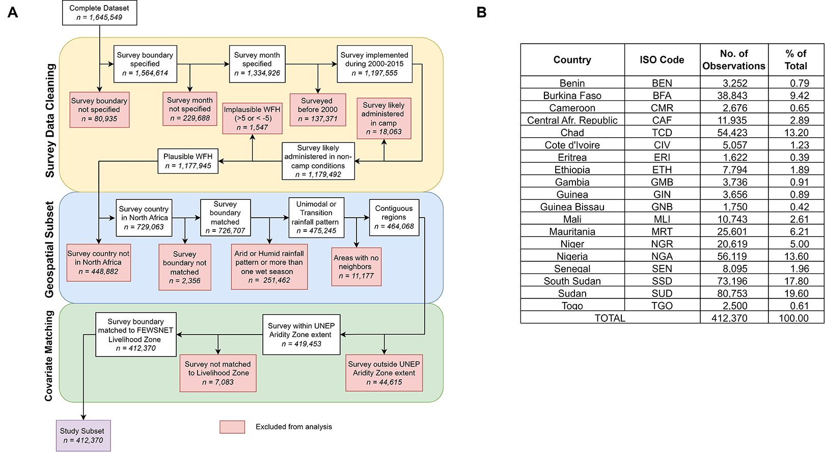
Data processing workflow and summary. (A) Flowchart of data cleaning process. (B) Observations and percentage of SMART surveys by country.

First, only observations with at least a level 1 administrative boundary and the month of survey were retained to ensure that the survey could be matched to a representative boundary and time for environmental data extraction. Data before year 2000 were also excluded due to extreme sparsity. A field was added to the data to identify whether the survey was conducted in an IDP or refugee camp based on the reported administrative regions and temporal information. These observations were removed since individuals in these settings rely on humanitarian aid and thus subject to less seasonality.^40,41 Observed GAM may also be artificially high in these settings due to population displacement and extreme asset depletion. Further corrections were made to remove extreme values for weight-for-height z-scores (WHZ), defined as WHZ >5 or WHZ <−5. These observations indicate inaccurate or extremely unlikely anthropometric measurements, which may introduce error in further estimates of GAM.

Geospatial Subset

Each survey was then matched to a corresponding level 1 or level 2 administrative boundary shapefile based on the provided spatial extent. A level 1 boundary is the largest subnational administrative unit of a country, and level 2 is the second largest, for example, state and county, respectively, in the United States. Each survey region was matched to the respective administrative boundary shapefile sourced from the Food and Agriculture Organization (FAO) Global Administrative Unit Layers (GAUL) data set⁴² or the Global Administrative Boundary Database (GADM).⁴³ If no match was found, a third attempt was made to match the survey region to a boundary shapefile closest to the year of the SMART survey from the US Agency for International Development (USAID) Demographic and Health Survey (DHS) Spatial Data Repository.⁴⁴ If no matches were found, the spelling of the survey region was investigated and, in some instances, corrected to once again match available feature names in GAUL, GADM, and DHS shapefiles. In some instances, the survey boundaries provided level 3 or town-level information and had to be corrected to match the correct level 2 administrative boundary based on a Google query. If no spatial boundaries were matched after this correction, the observations from the unmatched survey were excluded. Finally, noncontiguous survey regions were removed to ensure homogeneity in the study area.

Once a geospatial boundary was matched to each survey, the dominant rainfall pattern in the region was extracted using a geospatial overlay.⁴⁵ Administrative boundaries with primarily bimodal, multimodal, and humid rainfall patterns were excluded from the analysis. Since there was often a spatial mismatch between political boundaries and climatic boundaries, administrative areas comprising both arid and unimodal regions were considered transition regions and retained in this analysis (Figure 2, panel B). The following R packages were utilized for spatial analysis: rgdal,⁴⁶ rgeos,⁴⁷ raster,⁴⁸ tmap,⁴⁹ spdep,⁵⁰ and sf.⁵¹

Figure 2.

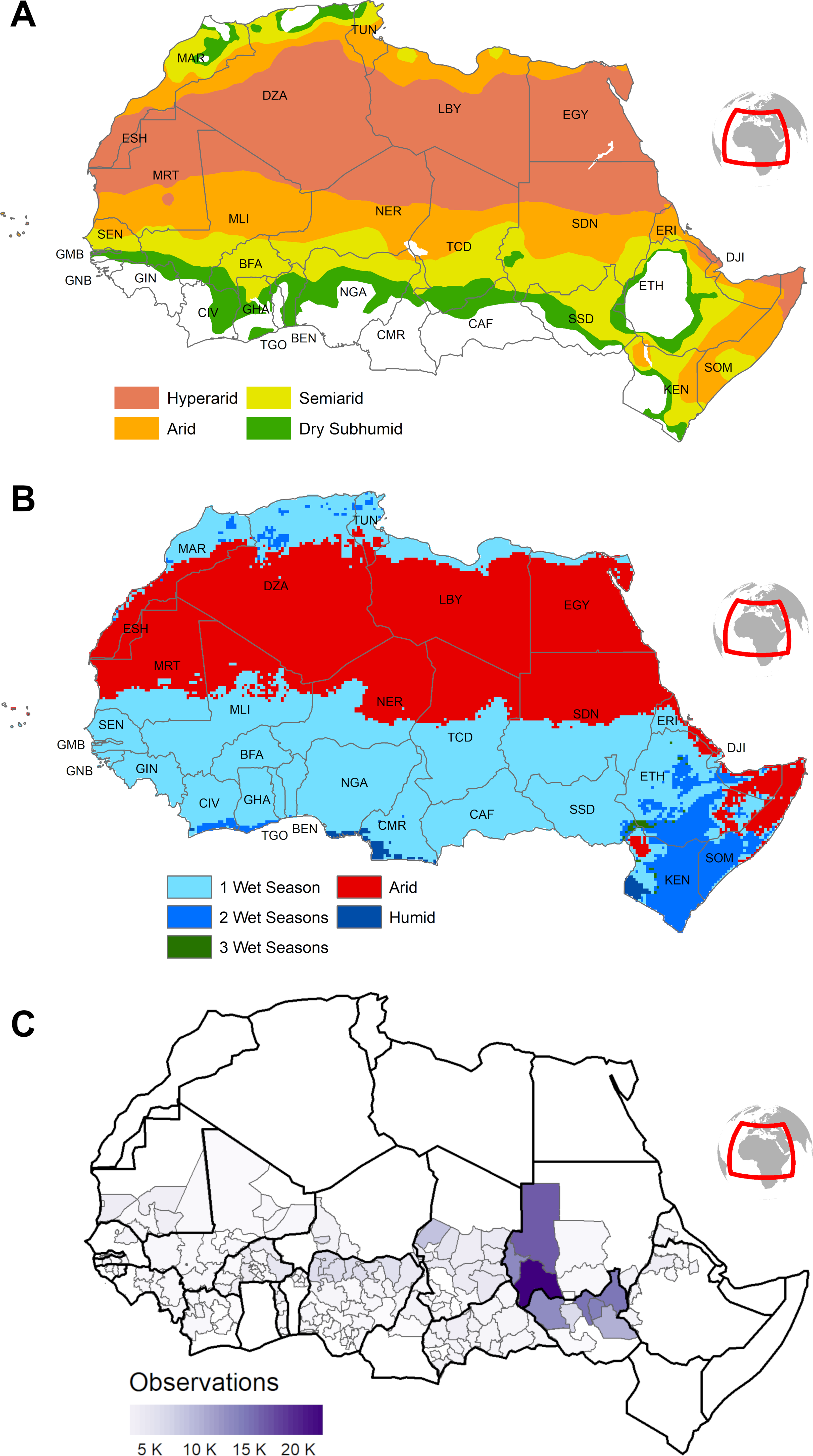
Maps of spatial extent. (A) UNEP aridity zone classification. (B) Rainfall patterns (Hermann and Mohr, 2011). (C) Total observations by SMART survey administrative boundaries.

Covariate Extraction

Aridity zones were extracted from the 2015 update to the United Nations Environment Programme (UNEP) delineation of global drylands.⁵² This data set classifies global drylands into 4 zones based on aridity index: hyperarid, arid, semiarid, and dry subhumid. Each survey extent shapefile was intersected with the UNEP aridity zone shapefile and assigned the aridity zone affecting the largest area (Figure 2, panel A).

Livelihood zones were defined based on the Famine Early Warning Systems Network (FEWSNET) livelihoods classification for priority countries.⁵³ This shapefile provides country-level spatial extents with a variety of details regarding agro-climatology, topography and elevation, land cover, food sources, and income-generating activities.⁵³ Examples of source livelihoods in the study area include western floodplain sorghum and cattle (South Sudan); northeast Sahelian millet, sesame, cowpeas, and livestock (Nigeria); and central agropastoral (Chad). The FEWSNET livelihood zone data set was developed from consultations with food security stakeholders and country experts.^53,54 Thus, it may fail to capture inter- and intracommunity heterogeneity in livelihoods as well as regional transitions toward mixed livelihood systems reflected in household survey data.^55,56 To reduce dimensionality, livelihood descriptions were used to classify each zone as primarily Agricultural, Agro-Pastoral, or Pastoral. Despite the loss of nuance in these constructed categories, the difference in GAM prevalence across communities led to the consideration of a livelihood dimension in this analysis.^5,20 The FEWSNET Country Livelihood Zone Reports were utilized for manual classification where livelihood zone names were ambiguous. Fishing-based livelihoods were excluded as they may follow different seasonal cycles compared to traditional agriculture.

The aggregated livelihoods zone shapefile was then intersected with each survey boundary shapefile, and the dominant livelihood type for each survey was calculated based on zone area. Given the target population of the SMART survey, it was determined that surveys on truly nomadic, pastoral populations are highly unlikely despite FEWSNET data indicating that surveyed regions practiced pastoral livelihoods. Therefore, regions initially classified as Pastoral based on FEWSNET descriptions were reclassified as Agro-Pastoral to account for the SMART surveys being implemented in primarily sedentary settings. Therefore, this analysis broadly studies differences between only agricultural and agro-pastoral livelihoods.

Matched administrative boundaries for each survey allowed for extraction of temperature, precipitation, and Normalized Differenced Vegetation Index (NDVI) covariates from gridded data sources. Temperature was extracted from TerraClimate,⁵⁷ precipitation from the Climate Hazards Group InfraRed Precipitation with Station data (CHIRPS) data set,⁵⁸ and NDVI from the National Aeronautics and Space Administration’s Vegetation Index and Phenology (VIP) data set.⁵⁹ Mean monthly values of temperature, precipitation, and NDVI were extracted for each survey boundary for each month in the complete study period of 2000 to 2015. Mean environmental measures from the month of survey were utilized for sensitivity analysis, whereas the 15-year time series was used to characterize the seasonal patterns of each covariate alongside the estimated GAM curve.

Peak Timing of Wasting

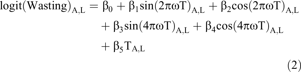
After data cleaning, a binary variable was created for wasting per the World Health Organization (WHO) anthropometric and clinical cutoffs.^2,60 A harmonic logistic regression was implemented to model child-level wasting. The inclusion of the first and second harmonic terms allows for the identification of a potential secondary peak in a calendar year. This formulation is shown in Equation 1, where Wasting is binary and T is the month of survey as a sequence of months in the study period. Linear, quadratic, and cubic trends were tested to accommodate fluctuations in wasting over time, perhaps driven by protracted crises or more frequent SMART survey implementation for monitoring purposes in recent years.

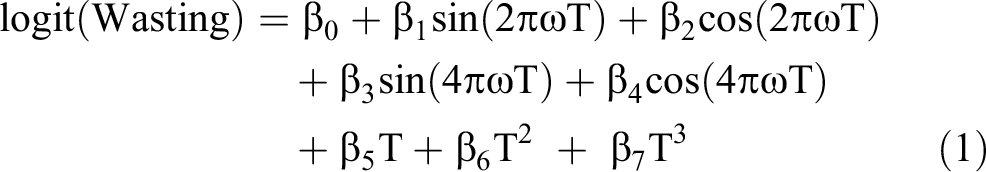
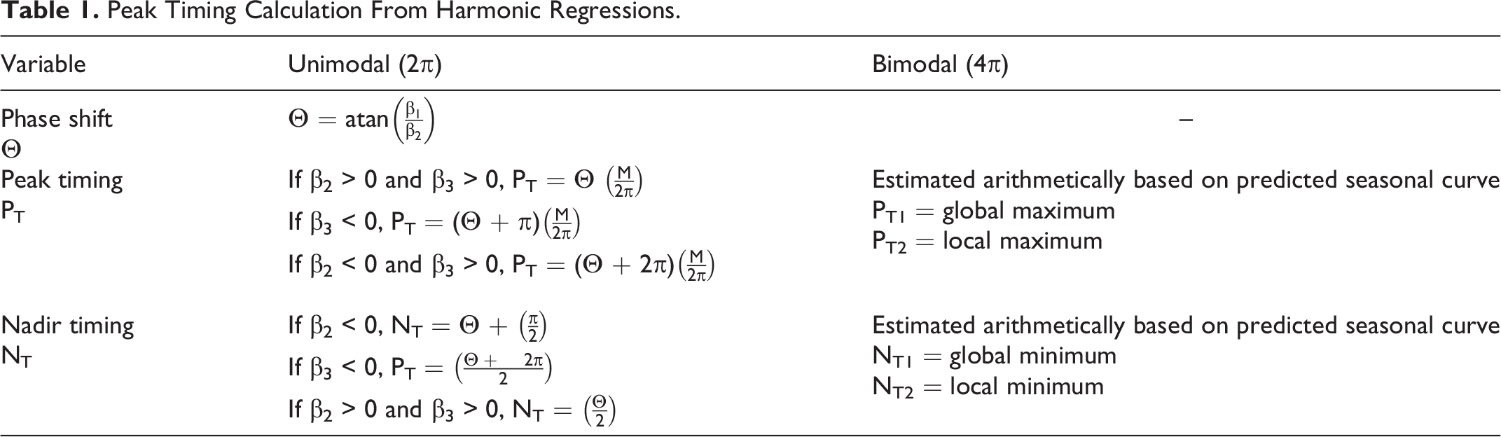
logit (Wasting) = β_{0} + β_{1} sin (2 πωT) + β_{2} cos (2 πωT) + β_{3} sin (4 πωT) + β_{4} cos (4 πωT) + β_{5} T + β_{6} T^{2} + β_{7} T^{3}

Equation 1 allows for the estimation of peak timing of child wasting depending on whether the second harmonic terms were statistically significant. If either of the second harmonic terms were statistically significant, the bimodal formulation was used to calculate peak timing; otherwise, the unimodal formulation was used (Table 1).

Table 1.

Peak Timing Calculation From Harmonic Regressions.

Variable	Unimodal (2π)	Bimodal (4π)
Phase shift Θ	Θ = atan $(\frac{β_{1}}{β_{2}})$	–
Peak timing P_T	If β₂ > 0 and β₃ > 0, P_T = Θ $(\frac{M}{2 π})$ If β₃ < 0, P_T = (Θ + π) $(\frac{M}{2 π})$ If β₂ < 0 and β₃ > 0, P_T = (Θ + 2π) $(\frac{M}{2 π})$	Estimated arithmetically based on predicted seasonal curve P_T1 = global maximum P_T2 = local maximum
Nadir timing N_T	If β₂ < 0, N_T = Θ + $(\frac{π}{2})$ If β₃ < 0, P_T = $(\frac{Θ + 2 π}{2})$ If β₂ > 0 and β₃ > 0, N_T = $(\frac{Θ}{2})$	Estimated arithmetically based on predicted seasonal curve N_T1 = global minimum N_T2 = local minimum

Equation 2 was used to study the peak timing of wasting across different aridity zones (Z) and livelihood zones (L) in the study area

logit {(Wasting)}_{A, L} = β_{0} + β_{1} sin {(2 πωT)}_{A, L} + β_{2} cos {(2 πωT)}_{A, L} + β_{3} sin {(4 πωT)}_{A, L} + β_{4} cos {(4 πωT)}_{A, L} + β_{5} T_{A, L}

Seasonality Analysis

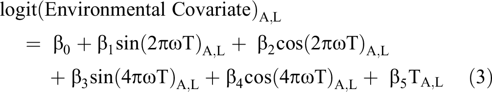
Equation 3 was utilized to estimate the peak and nadir timings of temperature, precipitation, and NDVI per Table 1 using the 15-year time series. These features were visualized alongside the estimated seasonal wasting curve to investigate temporal alignment across environmental and human factors.

logit {(Environmental Covariate)}_{A, L} = β_{0} + β_{1} sin {(2 πωT)}_{A, L} + β_{2} cos {(2 πωT)}_{A, L} + β_{3} sin {(4 πωT)}_{A, L} + β_{4} cos {(4 πωT)}_{A, L} + β_{5} T_{A, L}

[https://fic.tufts.edu/research-item/acute-malnutrition-seasonality-and-climate/].

Supplementary Analyses

Additional analyses were performed to study the robustness of observed seasonal patterns. First, the sensitivity of estimated coefficients to the inclusion of temperature, precipitation, and NDVI covariates across aridity and livelihood zones was examined. Next, the effect of data aggregation from individual-level wasting to survey-level GAM prevalence was investigated. These methods and results are detailed in Supplemental Information on our publicly available repository: [https://fic.tufts.edu/research-item/acute-malnutrition-seasonality-and-climate/].

Results

Study Extent

The geographic scope of this analysis is limited to 30 countries in the northern portion of the African continent classified by the United Nations Convention to Combat Desertification as drylands.⁵² This extent was chosen for its broad climatological similarity, as well as contextual knowledge of local seasonal patterns among the authors. The second criterion for inclusion in this study was unimodal rainfall pattern based on a simple temperature and precipitation-based classification scheme.⁴⁵ The final sample includes 412,370 observations from 561 SMART surveys in 19 countries. Characteristics of included surveys are summarized in Figure 1 (panel B), and a map of the study extent and observations is shown in Figure 2. A detailed discussion of SMART surveys is included in Supplemental Information on our publicly available repository: [https://fic.tufts.edu/research-item/acute-malnutrition-seasonality-and-climate/].

Descriptive Statistics

The link between climate and feasible livelihoods is evident in the low number of observations in the Arid, Agriculture partition (Figure 3). Majority of SMART surveys in this analysis were conducted in Semiarid regions (56% of all observations), followed by Dry Subhumid regions (25%). Temporal gaps in data collection are also apparent since the data set derives from selectively conducted rapid field surveys. SMART surveys in Arid, Agricultural areas were only conducted in 3 of 12 calendar months and inconsistently during the study period. This sparsity contrasts with data from Semiarid and Dry Subhumid regions, where SMART surveys were implemented consistently in the calendar year and frequently during the study period.

Figure 3.

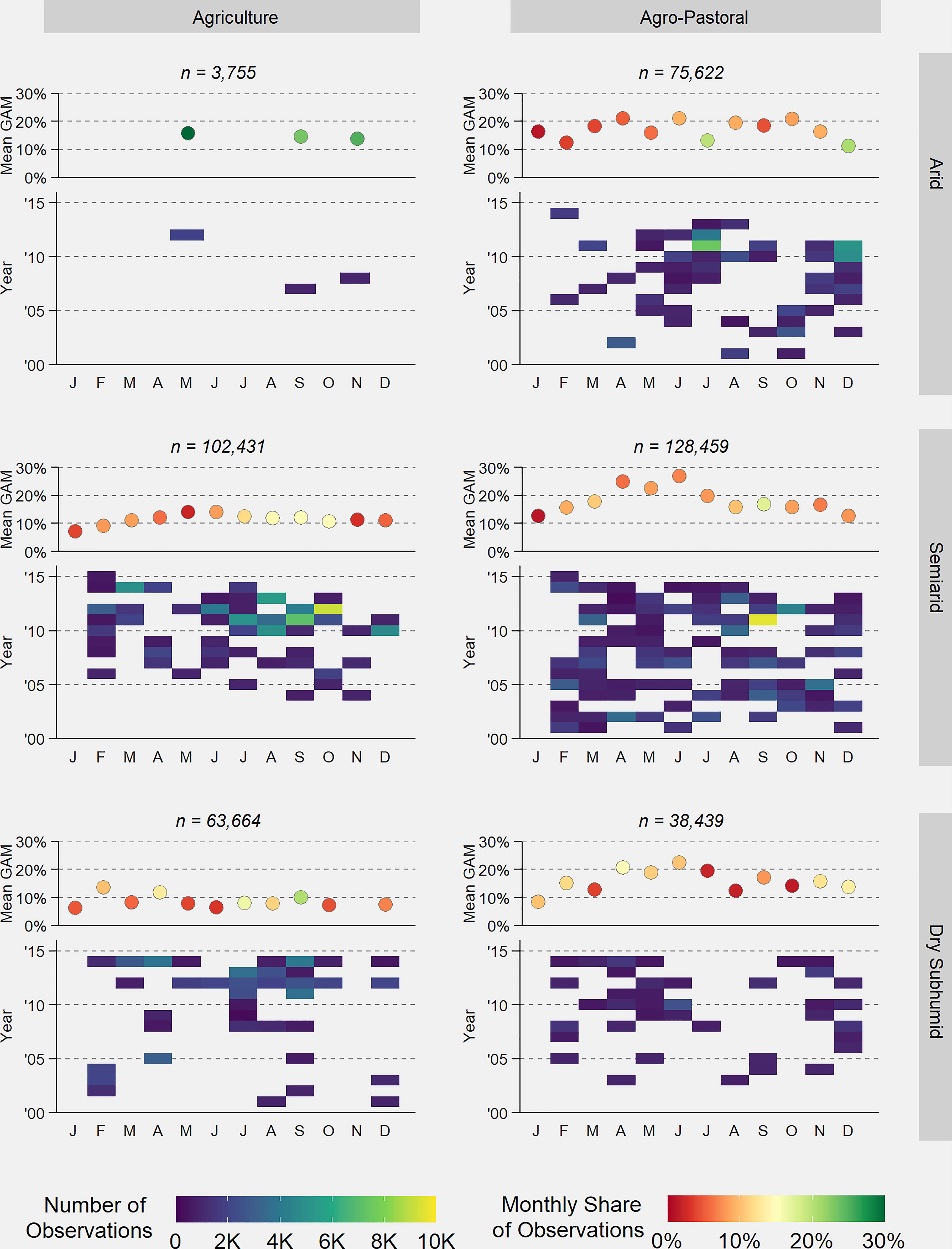
Distribution of observations and mean monthly prevalence of wasting, also known as global acute malnutrition (GAM). Data are presented by Aridity Zone (Arid, Semiarid, and Dry Subhumid) and Livelihood Zone (Agriculture, Agro-Pastoral). Each partition displays GAM by month (top), and a heatmap of the number of observations by month and year of SMART survey (bottom). Colors for mean GAM represent monthly share of observations per partition.

Estimating average GAM by month provides preliminary evidence of a seasonal pattern across all partitions (Figure 3). In Semiarid areas, GAM is greatest in April to June in both Agricultural and Agro-Pastoral communities. The shorter duration of higher GAM in Semiarid, Agro-Pastoral communities in November is also noticeable. This pattern is less clearly defined in Arid and Dry Subhumid regions in part due to smaller sample sizes. The observed variability in GAM serves as the foundation for further statistical modeling. Notably, months with highest mean GAM frequently comprise less than 15% of the share of observations. For example, in Semiarid Agricultural areas, the highest average GAM of 14.1% is observed in May; yet observations from May comprise only 6.9% of all observations in Semiarid Agricultural areas (n = 102,431). In all, 56.5% of observations in this partition are collected in July to October. This provides preliminary evidence that fewer SMART surveys may be conducted during periods of greatest vulnerability.

A high degree of variability in temperature, precipitation, and vegetation is observed across all regions (Figure 4). The rainy season generally lasts from June to September with maximum rainfall in August, although the magnitude of precipitation varies greatly across and within aridity zones. Highest temperatures are observed in April to May with a small warming period in September to November after peak rainfall. Cumulative greening is evident in NDVI, which generally peaks 1 to 2 months after cooling temperatures and increased precipitation. Lower NDVI in December to March indicates little plant growth, in line with postharvest dry season activities such as land preparation, fallowing, or grazing. GAM is highly variable across partitions but follows the temperature curve closely.

Figure 4.

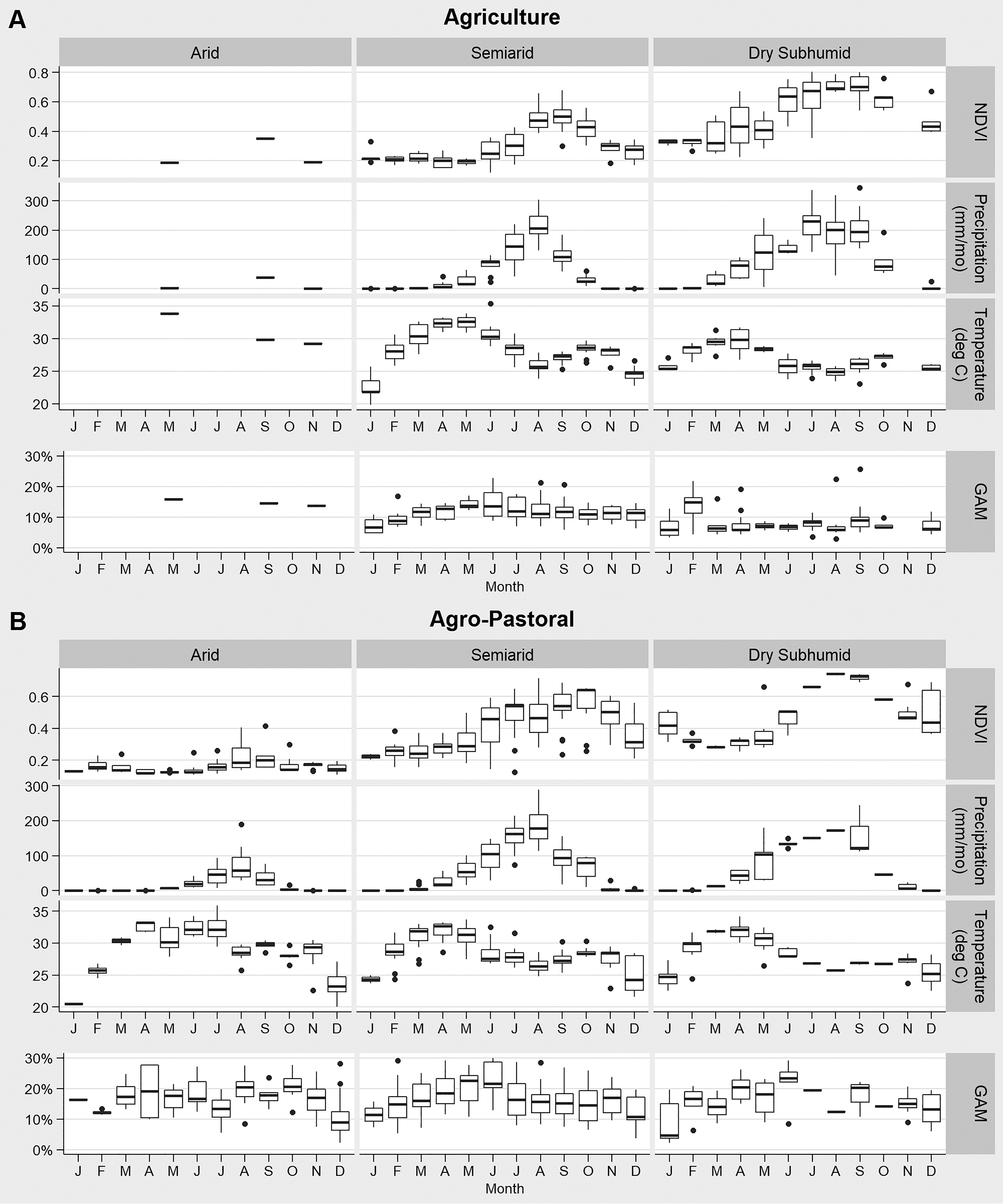
Boxplots of monthly mean environmental measures (NDVI, temperature, and precipitation) and GAM for aridity zones (Arid, Semiarid, and Dry Subhumid). Data are presented for (A) Agricultural and (B) Agro-Pastoral regions.

Peak Timing of Wasting

A simple bimodal harmonic logit with no trend term was used to predict wasting for the pooled data set (n = 412,370) (Figure 5). Peak timing of GAM is in mid-April, when estimated GAM reaches its highest peak of 19%. A second peak of 14% is observed in October. The nadir, or lowest value, for GAM prevalence is estimated in January (11%), and a local nadir is observed in early August (13%). Linear, quadratic, and cubic trends were tested to identify nonlinear trends in wasting over the study period. Only the linear trend was found to be statistically significant at the 1% level. Complete regression results are presented in Supplemental Information on our publicly available repository: [https://fic.tufts.edu/research-item/acute-malnutrition-seasonality-and-climate/].

Figure 5.

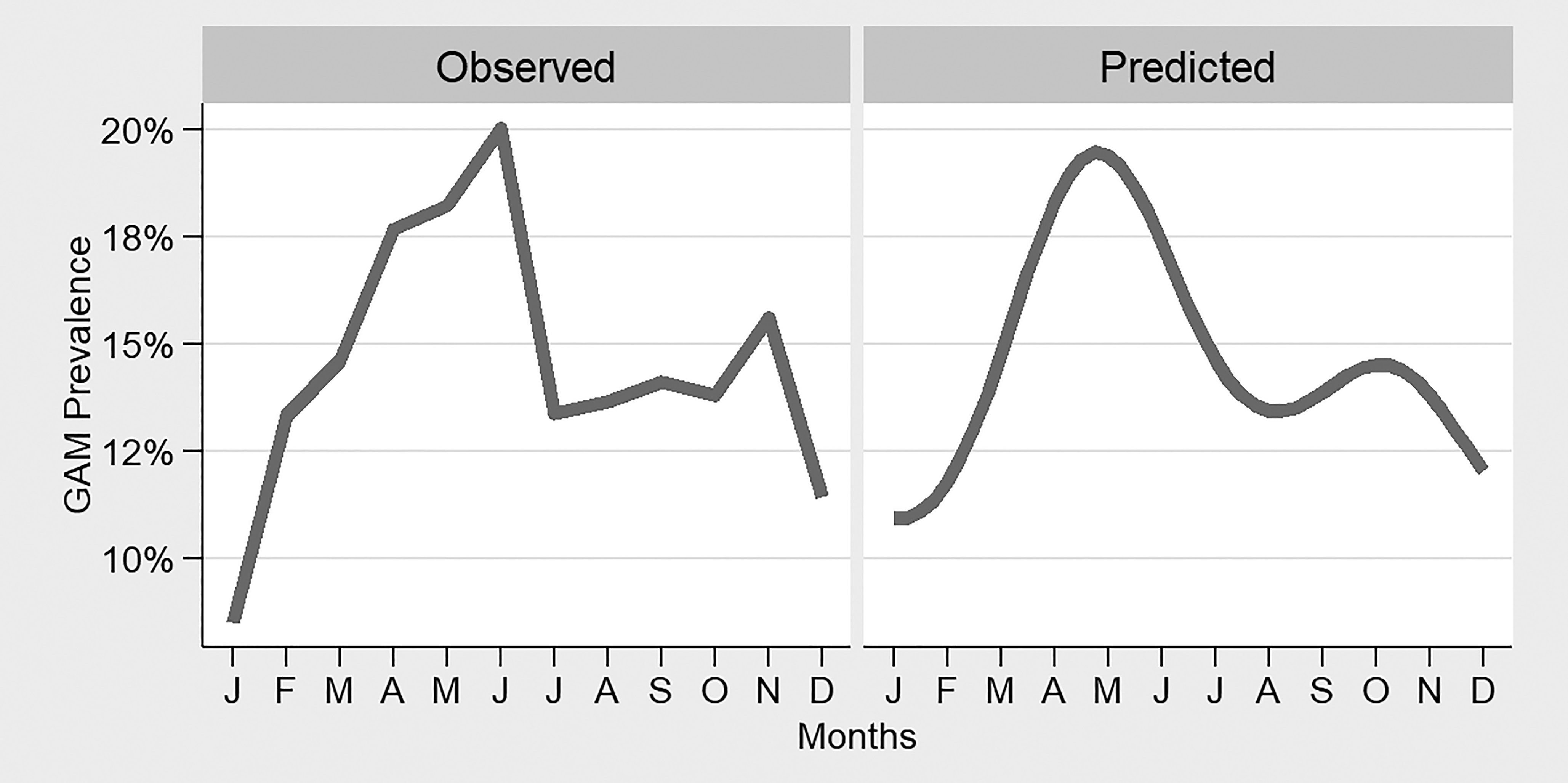
Monthly GAM prevalence in percentage for (A) observed mean and (B) predicted probability from total sample (n = 412,370).

Seasonality Analysis

The primary peak of GAM is consistently observed in April to May, with a second peak observed in Arid and Dry Subhumid regions in September to October (Figure 6). Although a mathematical secondary peak is not observed in Semiarid areas, a “shoulder” period of somewhat high prevalence is observed in September to October in both livelihood partitions. Across all partitions, primary peaks of wasting are closely aligned with primary peaks of temperature. Secondary peaks of wasting frequently follow the primary peaks of rainfall and NDVI in August to September. This period coincides with a secondary peak in temperature across all partitions in the study area.

Figure 6.

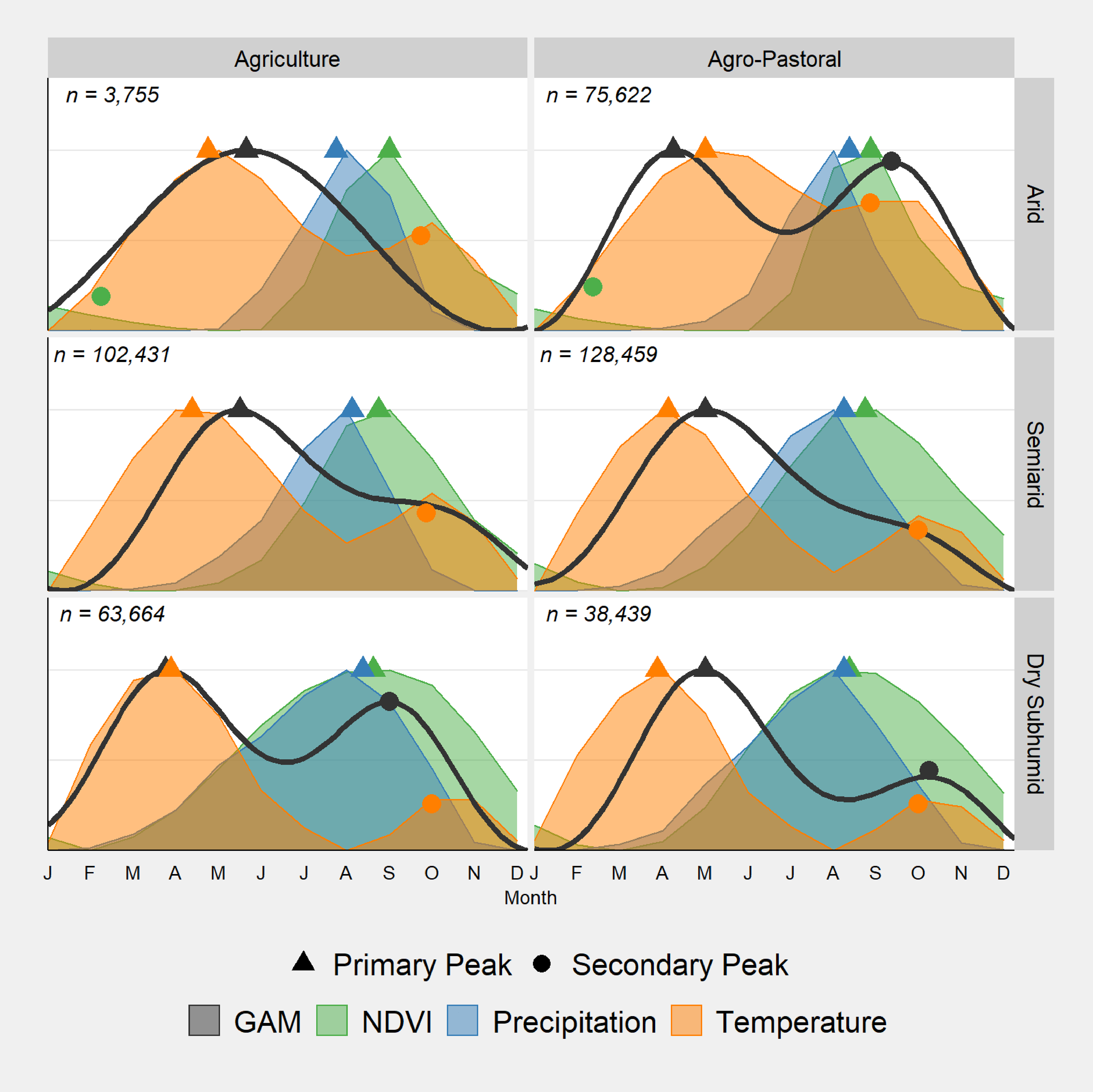
Scaled monthly mean temperature, precipitation, and NDVI overlaid with predicted harmonic GAM and estimated primary and secondary peaks for all variables.

Supplementary analyses indicate some variability in environmental factors, which may influence seasonal wasting, particularly in Dry Subhumid regions. The seasonal pattern of GAM is also stable across individual-level wasting and survey-level GAM prevalence outcomes. A complete discussion on the effect of aggregation across aridity and livelihood zones is presented in Supplemental Information on our publicly available repository: [https://fic.tufts.edu/research-item/acute-malnutrition-seasonality-and-climate/].

Discussion

A robust analysis of 15 years of SMART surveys (n = 412,370) confirms a bimodal pattern, or the presence of 2 distinct peaks of wasting during the calendar year in the African drylands. Although the preharvest hungry season in August to September is traditionally considered the peak of acute malnutrition, empirical results indicate that this is actually the secondary peak of wasting during the calendar year. The greatest magnitude of wasting is observed in April to May across all partitions and is consistently aligned with the primary peak of temperature. The secondary peak of wasting in September to October aligns with primary peaks of rainfall and NDVI and the secondary peak of temperature (Figure 6), indicating complex climate at play alongside human factors.

This empirical analysis proves that the hungry season assumption has conflated the primary and secondary peaks of wasting in African drylands. Greater focus on the secondary wasting peak in September to October has led to a “blind spot” for the primary peak of wasting in April to May, which should be the period of greatest concern for relevant nutrition programming. Despite the importance of the primary peak, less than 15% of surveys in the SMART data set were implemented in April to May. Instead, SMART surveys are most frequently conducted in preharvest months of July to September, which comprise approximately 34% of surveyed months in this data set. The focus on survey timing during the secondary peak of wasting is particularly pronounced in Agricultural areas, where only 12% of surveys are implemented during April or May (Figure 7). Insufficient data collection during peak hunger months can misinform intervention timing and mislead monitoring and evaluation efforts. Although uneven data collection can potentially bias the seasonal patterns observed in the SMART data set, greater survey frequency during April to May can help validate the estimated seasonal pattern of wasting.

Figure 7.

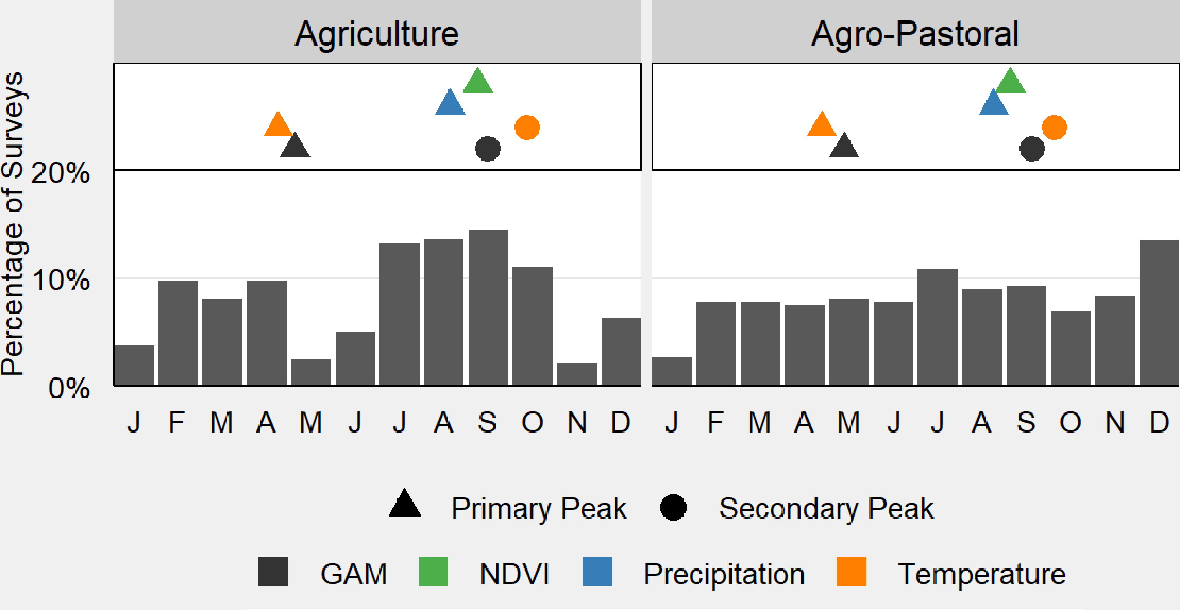
Primary and secondary peaks of wasting prevalence (GAM), temperature, precipitation, and NDVI, alongside histograms of survey frequency in Agricultural and Agro-Pastoral livelihood zones.

The varied seasonal patterns of wasting observed in this analysis highlight environmental seasonality as a critical basic determinant of acute malnutrition in African drylands.^6,35 Our findings underline the need for greater emphasis on the basic causes of child malnutrition, including environmental variability, livelihoods, and institutions.³⁵ Dryland production systems depend on environmental resources (rangeland, farmland, water, and forest resources, for example) that are seasonally distributed with variable availability in space and time. Formal and informal institutions play a crucial role in managing these resources and mediating access, which in turn determines the underlying drivers of malnutrition. Environmental variability also directly affects availability, access, and utilization of basic services and accelerates pathways to malnutrition through infectious disease cycles and asset losses in case of extreme weather events. Therefore, nutrition analyses among dryland populations must be complemented with analyses of climate as a critical upstream determinant of acute malnutrition and its drivers. Joint studies are particularly relevant in the context of climate change, which is expected to worsen water scarcity and accelerate desertification in African drylands.^61,62

This study also exemplifies key methodological considerations for the study of seasonality. Aggregation of day, week, and month variables into broad seasons can introduce significant bias in seasonality analyses. The hungry season hypothesis and resulting hungry/lean season dichotomies have undoubtedly influenced countless survey designs and instruments over the past decades. While the single-peak hunger season cycle may be true in some areas, generalizing these conclusions to the drylands and other climatic zones requires a rigorous examination of existing data using continuous temporal variables rather than discretized simplifications such as dry/wet season or pre-/postharvest. These categories are constraining and often inaccurate, as we find that the approximate preharvest survey period in the SMART data set with highest frequency of observations overlooks the primary peak of wasting. Analytically, harmonic regression applications must include second- and higher order harmonics to test the possibility of more than one peak, regardless of the seasonal pattern of environmental variables. This analysis demonstrates that one wet season, or a unimodal rainfall pattern, does not imply unimodal pattern of wasting. More robust analyses of environmental seasonality are thus necessary in nutrition survey design and analysis.

The peak timing of wasting was observed to be similar across livelihood zones in this study (Figure 6). This similarity may be driven by the low spatial resolution of the FEWSNET Livelihood Zones source data, which treats livelihood zones as geographically distinct production systems instead of overlapping and integrated practices. Households specializing in different livelihoods often live in close proximity,⁵⁵ and primary data indicate a long-term transition toward mixed livelihood systems in the study area.⁵⁶ These household- and region-specific nuances may be lacking in the FEWSNET Livelihood Zone classification, which aggregates across similar production systems, income choices, and trade options to inform its country-level livelihoods analysis.⁵⁴ Despite this limitation, the constructed livelihood categories utilized in this article allow us to interrogate existing assumptions of seasonal patterns by livelihoods rather than establishing them. Future studies utilizing spatial data on livelihood zones are advised to validate classifications with household-level primary data and qualitative inquiry to obtain an accurate profile of livelihood specializations in the study region.

This analysis further highlights the utility of secondary data for nuanced analyses beyond population-level trends. High-frequency primary data collection on nutrition outcomes is rare due to high costs and logistical constraints. Remote dryland communities are often not captured in routine national surveys due to low population densities, lack of accessible roads, seasonal migration patterns of pastoralists, and lack of health and administrative infrastructure. Populations at risk of humanitarian crises are better represented in rapid nutrition assessments and early warning systems, which aim to inform humanitarian action. Survey and needs assessment data from vulnerable populations in these domains are abundant, and this analysis demonstrates the utility of these data far beyond a simple snapshot in time as currently utilized. The SMART data set demonstrates the richness of readily available secondary data and the value that can be gleaned when combined with other secondary data sources.

Despite its utility for nutrition research, the SMART data set has several limitations, which must be acknowledged. First, SMART surveys are rapid assessment tools that are not designed for surveillance. Results from SMART surveys, and therefore this analysis, have limited external validity and are not representative of overall acute malnutrition in their respective regions. Interpretations of our results must, therefore, focus on the variability of GAM patterns rather than the estimated magnitude of GAM across climatological and livelihood partitions. Data quality is also a key consideration in this analysis. The accuracy and veracity of the spatial fields determined the accuracy of our results; consequently, a degree of spatial uncertainty is to be expected. The source data set did not indicate whether a survey was implemented in a refugee or internally displaced persons camp, so this field was manually matched based on the region and district fields. Surveys that could not be matched to a verifiable camp location were included in this analysis. This decision rule explains the inclusion of several surveys from North Darfur and Eastern Equatoria states (Figure 2). Changing data selection criteria will likely modify seasonality estimates; however, we expect the seasonal patterns to be robust in climatologically similar regions of Africa.

Several simple solutions can improve SMART data accessibility and inform future primary data collection for seasonality analysis. The SMART data, like most surveys, are now collected using digital devices that automatically record temporal information. Reporting the day of data collection along with survey month would allow for more precise seasonality analysis. The SMART surveys may also record spatial information such as GPS points or community boundaries where explicitly provided permission to collect these data. Sharing spatial data with permitted users can further build expertise on the spatiotemporal variability of malnutrition. A centralized deidentified SMART survey repository with a public-facing dashboard is an ideal solution for maximum transparency and interagency coordination in humanitarian contexts. Such a repository is currently being developed by Action Against Hunger Canada and will serve as a critical tool for streamlined high-resolution analysis of SMART data. Beyond data management, short periods of high-frequency SMART surveys in key regions can potentially help establish baseline seasonality of key indicators and identify optimum survey timing for improved nutrition surveillance.

Extensions of seasonality analysis beyond the SMART data set are also necessary to document global variability in acute malnutrition patterns. Presented methods can be easily applied to longitudinal surveys with at least monthly observations. In regions with 2 or more wet seasons, harmonic regression should include higher order harmonics to ensure that all statistically significant seasonal patterns are being captured. Data quality for seasonality analysis can be drastically improved by incorporating multiple survey rounds in different months, environmental measurements, and GPS information in primary data collection. Further research is also required to study the individual, household, communal, institutional, and environmental drivers of the observed bimodal wasting pattern. Seasonal patterns from this analysis can be readily compared to seasonal admissions to therapeutic feeding programs for cross-validation.

Further methodological improvements can more precisely estimate seasonal patterns through covariates regarding the availability, access, and utilization of basic services, as well as other secondary data on population density, road networks, markets, terms of trade, elevation, conflict, and extreme weather events. Future analyses can also apply harmonic regression methods to other nutrition outcomes such as severe and moderate acute malnutrition, as well as other body composition and anthropometric measures such as mid-upper arm circumference, weight-for-height, and height-for-age. Household-level data can augment existing spatial data on overlapping livelihood specializations and add necessary nuance to future studies on seasonality of acute malnutrition across livelihoods. Qualitative and mixed methods can more accurately capture complex production systems and livelihoods and potentially incorporate factors related to social equity such as gender and socioeconomic class. Such investigations can provide key insights into varied dimensions of acute malnutrition seasonality and contribute to achieving the global goal of ending hunger through good nutrition for all.

Conclusion

Secondary analysis of 15 years of SMART survey data indicates that there are 2 peaks of wasting in African drylands. The primary peak is observed in April to May, coinciding with the primary peak of temperature. A secondary period of higher wasting prevalence is observed in September to October, coincident with the primary peaks of precipitation and NDVI and the secondary peak of temperature. Seasonality analysis must, therefore, utilize continuous time instead of discrete seasons to capture this variability during the calendar year. Harmonic regressions must also be correctly specified to allow for the possibility of 2 or more peaks where statistically significant. Greater survey frequency during primary peak months can improve knowledge regarding wasting trends and differential drivers of wasting during the calendar year. Prevalence estimates of wasting, particularly from cross-sectional surveys, must be interpreted within the context of this seasonal pattern.

Supplemental Material

Supplemental Material, sj-pdf-1-fnb-10.1177_03795721231178344 - Seasonality of Acute Malnutrition in African Drylands: Evidence From 15 Years of SMART Surveys

Supplemental Material, sj-pdf-1-fnb-10.1177_03795721231178344 for Seasonality of Acute Malnutrition in African Drylands: Evidence From 15 Years of SMART Surveys by Aishwarya Venkat, Anastasia Marshak, Helen Young and Elena N. Naumova in Food and Nutrition Bulletin

Footnotes

Authors’ Note

Aishwarya Venkat, Anastasia Marshak, Helen Young, and Elena N. Naumova contributed equally to this work. The secondary analysis presented herein utilized a compilation of SMART surveys. These surveys were originally implemented by several nongovernmental organizations and United Nations agencies to estimate prevalence of food insecurity and undernutrition in emergency and development settings.^21,36 Any identifying data collected for programmatic purposes such as recruitment of acutely malnourished children into feeding programs were removed by implementing organizations prior to data sharing, and the authors received exclusively deidentified data. No experiments were performed on human participants during SMART data collection or in subsequent secondary analyses.^21,36 No permissions were requested or provided for this study as it performed secondary analysis on already collected and deidentified SMART survey data.

A complete list of nongovernmental organizations and United Nations agencies that implemented SMART data collection is provided by Myatt et al.³⁶ The authors were not involved in the design or implementation of any of the SMART surveys included in this analysis. Requisite permissions and approvals for SMART data collection by the respective agencies were sought from and provided by the relevant international and/or national authorities, including United Nations coordinating body, Ministry of Health, the government bodies responsible for humanitarian action, and also government and/or rebel authority security bodies. Participation in SMART surveys was voluntary, and child anthropometry was only collected after provision of verbal informed consent from the primary caregiver of the child. Written consent was not sought due to low rates of literacy among respondents. The existence of data is proof of consent.^21,36 All other data utilized in this analysis derive from publicly accessible sources.

Acknowledgments

The authors extend gratitude to Mark Myatt (Brixton Health, Wales, UK) and team for sharing the foundational compilation of SMART surveys for this publication. The authors also thank Stefanie Herrmann (The University of Arizona, Arizona, USA) and Karen Mohr (Goddard Space Flight Center, National Aeronautics and Space Administration, Maryland, USA) for sharing the continental rainfall modality classification spatial data.

Declaration of Conflicting Interests

The author(s) declared no potential conflicts of interest with respect to the research, authorship, and/or publication of this article.

Funding

AV and ENN were supported in part by The Office of the Director of National Intelligence (ODNI), Intelligence Advanced Research Projects Activity (IARPA), via 2017-17072100002. The views and conclusions contained herein are those of the authors and should not be interpreted as necessarily representing the official policies, either expressed or implied, of ODNI, IARPA, or the US Government. The US Government is authorized to reproduce and distribute reprints for governmental purposes. ENN was supported in part by the US National Science Foundation Grant IGE # 1855886 SOLution-oriented, STudent-Intiated, Computationally-Enriched (SOLSTICE) Training. The funders had no role in study design, data collection and analysis, decision to publish, or preparation of the manuscript.

Supplemental Material

Supplemental material for this article is available online.

Note

References

UN. The Sustainable Development Goals Report 2020. UN; 2020.

WHO, UNICEF. WHO Child Growth Standards and the Identification of Severe Acute Malnutrition in Infants and Children. WHO and UNICEF; 2009.

UNICEF, WHO, IBRD/WB. Levels and Trends in Child Malnutrition: Key Findings of the 2020 Edition of the Joint Child Malnutrition Estimates. World Health Organization; 2020.

FAO, IFAD, UNICEF, WFP, WHO. The State of Food Security and Nutrition in the World 2020: Transforming Food Systems for Affordable Healthy Diets. FAO; 2020.

Chotard

Mason

Oliphant

Mebrahtu

Hailey

. Fluctuations in wasting in vulnerable child populations in the greater horn of Africa. Food Nutr Bull. 2010;31(3):S219–S233.

Vaitla

Devereux

Swan

. Seasonal hunger: a neglected problem with proven solutions. PLoS Med. 2009;6(6):e1000101.

Baye

Hirvonen

. Seasonality: a missing link in preventing undernutrition. Lancet Child Adolesc Health. 2020;4(1):e3.

FAO and Tufts University. Twin Peaks: The Seasonality of Acute Malnutrition, Conflict and Environmental Factors—Chad, South Sudan and the Sudan. 2019.

Pelletier

Deneke

Kidane

Haile

Negussie

. The food-first bias and nutrition policy: lessons from Ethiopia. Food Policy. 1995;20(4):279–298.

10.

Chambers

. Introduction. In: Chambers

Longhurst

Pacey

, eds. Seasonal Dimensions to Rural Poverty . IDS; 1981.

11.

Teokul

Payne

Dugdale

. Seasonal variations in nutritional status in rural areas of developing countries: a review of the literature. Food Nutr Bull. 1986;8(4):7–10.

12.

Ferro-Luzzi

Branca

. Nutritional seasonality: the dimensions of the problem. In: Ulijaszek

Strickland

, eds. Seasonality and Human Ecology. Society for the Study of Human Biology Symposium Series. Cambridge University Press; 1993:149–165.

13.

UNICEF. Improving Child Nutrition: The Achievable Imperative for Global Progress. United Nations Children’s Fund; 2013.

14.

Egata

Berhane

Worku

. Seasonal variation in the prevalence of acute undernutrition among children under five years of age in east rural Ethiopia: a longitudinal study. BMC Public Health. 2013;13:864.

15.

Grellety

Luquero

Mambula

Adamu

Elder

Porten

. Observational bias during nutrition surveillance: results of a mixed longitudinal and cross-sectional data collection system in Northern Nigeria. PLoS One. 2013;8(5):e62767.

16.

Chikhungu

Madise

. Seasonal variation of child under nutrition in Malawi: is seasonal food availability an important factor? Findings from a national level cross-sectional study. BMC Public Health. 2014;14:1146.

17.

Martin-Canavate

Custodio

Yusuf

Molla

Fasbender

Kayitakire

. Malnutrition and morbidity trends in Somalia between 2007 and 2016: results from 291 cross-sectional surveys. BMJ Open. 2020;10(2):e033148.

18.

Sadler

Mitchard

Abdi

Shiferaw

Bekele

Catley

. Milk Matters: The Impact of Dry Season Livestock Support on Milk Supply and Child Nutrition in Somali Region, Ethiopia. Feinstein International Center, Tufts University & Save the Children. 2012. Accessed November 16 2022. https://fic.tufts.edu/wpcontent/uploads/Milk-Matters-2.pdf

19.

Marshak

Venkat

Young

Naumova

. How seasonality of malnutrition is measured and analyzed. Int J Environ Res Public Health. 2021;18(4):1828.

20.

Bechir

Schelling

Bonfoh

, et al. Evolution saisonnière du statut nutritionnel des enfants nomades et sédentaires de moins de cinq ans dans le Sahel au Tchad. Med Trop. 2010;70:353–358.

21.

Isanaka

Boundy

Grais

Myatt

Briend

. Improving estimates of numbers of children with severe acute malnutrition using cohort and survey data. Am J Epidemiol. 2016;184(12):861–869.

22.

SMART. Standardized Monitoring and Assessment for Relief and Transitions (SMART) Manual 2.0. Technical Advisory Group; 2017.

23.

Cameron

Trivedi

. Regression Analysis of Count Data London. Cambridge University Press; 2013.

24.

Lofgren

Fefferman

Doshi

Naumova

Assessing Seasonal Variation in Multisource Surveillance Data: Annual Harmonic Regression; Springer Berlin Heidelberg; 2007.

25.

Bhaskaran

Gasparrini

Hajat

Smeeth

Armstrong

. Time series regression studies in environmental epidemiology. Int J Epidemiol. 2013;42(4):1187–1195.

26.

Ramanathan

Thenmozhi

George

, et al. Assessing seasonality variation with harmonic regression: accommodations for sharp peaks. Int J Environ Res Public Health. 2020;17(4):1318.

27.

Naumova

MacNeill

. Seasonality assessment for Biosurveillance systems. In: Auget

Balakrishnan

Mesbah

Molenberghs

, eds. Advances in Statistical Methods for the Health Sciences: Applications to Cancer and AIDS Studies, Genome Sequence Analysis, and Survival Analysis. Birkhäuser Boston; 2007. 437–450.

28.

Jagai

Sarkar

Castronovo

, et al. Seasonality of rotavirus in South Asia: a meta-analysis approach assessing associations with temperature, precipitation, and vegetation index. PLoS One. 2012;7(5):e38168.

29.

Kulinkina

Mohan

Francis

, et al. Seasonality of water quality and diarrheal disease counts in urban and rural settings in south India. Sci Rep. 2016;6:20521.

30.

Stratton

Ehrlich

Mor

Naumova

. A comparative analysis of three vector-borne diseases across Australia using seasonal and meteorological models. Sci Rep. 2017;7(1):40186.

31.

Alarcon Falconi

Cruz

Naumova

. The shift in seasonality of legionellosis in the USA. Epidemiol Infect. 2018;146(14):1824–1833.

32.

Nielsen

Prudhon

de Radigues

.Trends in malnutrition and mortality in Darfur, Sudan, between 2004 and 2008: a meta-analysis of publicly available surveys. Int J Epidemiol. 2011;40(4):971–984.

33.

Saville

Cortina-Borja

De Stavola

, et al. Comprehensive analysis of the association of seasonal variability with maternal and neonatal nutrition in lowland Nepal. Public Health Nutr. 2021;25(7):1–16.

34.

Alarcon Falconi

Estrella

Sempértegui

Naumova

. Effects of data aggregation on time series analysis of seasonal infections. Int J Environ Res Public Health. 2020;17(16):5887.

35.

Young

. Nutrition in Africa’s Drylands: A Conceptual Framework for Addressing Acute Malnutrition. Feinstein International Center; 2020.

36.

Myatt

Khara

Schoenbuchner

, et al. Children who are both wasted and stunted are also underweight and have a high risk of death: a descriptive epidemiology of multiple anthropometric deficits using data from 51 countries. Arch Public Health. 2018;76:28.

37.

R Core Team. R: A Language and Environment for Statistical Computing. R Foundation for Statistical Computing; 2019.

38.

RStudio Team. RStudio: Integrated Development for R. RStudio, PBC; 2020.

39.

Wickham

. Tidyverse: Easily Install and Load the ‘Tidyverse’. R package version 1.2.1 ed; 2017.

40.

Darrouzet-Nardi

Masters

. Nutrition smoothing: can proximity to towns and cities protect rural children against seasonal variation in agroclimatic conditions at Birth? PLoS One. 2017;12(1):e0168759.

41.

Kim

Humphrey

Marshak

Gathuoy

Krishnan

. The Currency of Connections: Why Do Social Connections Matter for Household Resilience in South Sudan? Feinstein International Center, Tufts University; 2020.

42.

FAO. Global Administrative Unit Layers (GAUL); 2015.

43.

Global Administrative Areas (GADM). Database of Global Administrative Areas, Version 2.0; 2012.

44.

ICF. The DHS Program Spatial Data Repository; 2019.

45.

Herrmann

Mohr

. A continental-scale classification of rainfall seasonality regimes in Africa based on gridded precipitation and land surface temperature products. Appl Meteorol Climatol. 2011;50(12):2504–2513.

46.

Bivand

Keitt

Rowlingson

. rgdal: Bindings for the ‘Geospatial’ Data Abstraction Library. R package version 1.4-8 ed; 2019.

47.

Bivand

Rundel

. rgeos: Interface to Geometry Engine—Open Source (‘GEOS’). R package version 0.4-2 ed; 2018.

48.

Hijmans

. raster: Geographic Data Analysis and Modeling. R package version 2.9-1 ed; 2019.

49.

Tennekes

tmap: thematic maps in R. J Statis Software. 2018;84(6):1–39.

50.

Bivand

Pebesma

Gomez-Rubio

. Applied Spatial Data Analysis With R. 2nd ed. Springer; 2013.

51.

Pebesma

. Simple Features for R: Standardized Support for Spatial Vector Data. The R Journal; 2018.

52.

Sorensen

. A Spatial Analysis Approach to the Global Delineation of Dryland Areas of relevance to the CBD Programme of Work on Dry and Subhumid Lands. UNEP-WCMC; 2007.

53.

FEWS-NET. Livelihood Zones; 2018.

54.

Grillo

Holt

. Application of the Livelihood Zone Maps and Profiles for Food Security Analysis and Early Warning: Guidance for Famine Early Warning Systems Network (FEWS NET) Representatives and Partners. USAID FEWSNET; 2009.

55.

Marshak

Luc

Radday

Young

. Seasonality of Acute Malnutrition and Its Drivers in Sila Province, Chad: A Mixed Methods Analysis. Feinstein International Center, Tufts University; 2021. Accessed November 16 2022. https://fic.tufts.edu/wp-content/uploads/SeasonalityofAcuteMalnutChadFinal-1.pdf

56.

Young

Ismail

. Complexity, continuity and change: livelihood resilience in the Darfur region of Sudan. Disasters. 2019;43(suppl 3):S318–S344.

57.

Abatzoglou

Dobrowski

Parks

Hegewisch

. TerraClimate, a high-resolution global dataset of monthly climate and climatic water balance from 1958-2015. Sci Data. 2018;5:170191.

58.

Funk

Peterson

Landsfeld

, et al. The climate hazards infrared precipitation with stations—a new environmental record for monitoring extremes. Sci Data. 2015;2:150066.

59.

Didan

Barreto

. NASA MEaSUREs Vegetation Index and Phenology (VIP) Vegetation Indices Monthly Global 0.05Deg CMG. In: Eosdis

, ed. Land Processes DAAC; 2016.

60.

WHO. The Management of Nutrition in Major Emergencies. WHO, UNHCR, IFRC, WFP; 2000.

61.

Huang

, et al. Dryland climate change: recent progress and challenges. Rev Geophysics. 2017;55(3):719–778.

62.

Serdeczny

Adams

Baarsch

, et al. Climate change impacts in Sub-Saharan Africa: from physical changes to their social repercussions. Reg Environ Change. 2017;17(6):1585–1600.

Supplementary Material

Please find the following supplemental material available below.

For Open Access articles published under a Creative Commons License, all supplemental material carries the same license as the article it is associated with.

For non-Open Access articles published, all supplemental material carries a non-exclusive license, and permission requests for re-use of supplemental material or any part of supplemental material shall be sent directly to the copyright owner as specified in the copyright notice associated with the article.

0.00 MB

0.33 MB