Joint Latent Analysis of Behavioral Patterns in Multi-Source Origin

Abstract

Urban origin–destination (OD) data often come from two distinct sources: traditional surveys and global positioning system (GPS)-based records. The former offer rich behavioral detail but are infrequent and costly, while the latter provide continuous coverage but lack semantic context. They often lead to different findings and are rarely examined together, making it difficult to build a consistent understanding of urban travel behavior. To address this gap, we propose a dynamic joint latent factor model that decomposes multi-source OD matrices into shared spatial structures and source-specific temporal dynamics. The model identifies latent movement patterns by jointly factorizing both datasets while allowing each source to retain its unique temporal characteristics. Applied to GPS and survey OD data from Ottawa, Canada, the model achieves strong reconstruction accuracy ( $R^{2} \approx 0.8$ overall). The results uncover stable spatial patterns alongside clear differences in the traveler groups driving each latent mode. GPS factors emphasize younger and higher-income travelers, especially in the more flexible afternoon period. However, survey factors reflect routine commuting by middle-aged and middle-income households. These patterns show that the joint model isolates behavioral differences from sampling bias and provides a coherent representation of OD demand across sources. Together, these results show that the joint factorization quantifies behavioral differences from sampling bias and provides a coherent representation of OD demand across sources. This framework helps compare and interpret multi-source OD data in settings where traditional surveys are limited.

Keywords

Origin-destination matrices multi-source OD data GPS data household travel survey dynamic joint latent factor model low-rank factorization travel behavior patterns

Introduction

Origin–destination (OD) matrices are a cornerstone of urban transportation planning. They support critical analyses ranging from travel demand forecasting to infrastructure investment and modal share evaluation ( 1 – 3 ). Traditionally, OD matrices are derived from household travel surveys (HTS), which offer rich demographic and behavioral context ( 4 ). However, these surveys are costly and temporally sparse. In Canadian cities, for instance, they are often conducted only once every 5 years and typically fielded in the fall, which may limit representativeness across seasons and potentially introduce seasonal bias in mode shares and trip patterns ( 4 – 6 ). In recent years, alternative sources such as global positioning system (GPS) traces, mobile phone data, and transit smart cards have emerged, offering continuous and large-scale observations of mobility patterns ( 7 , 8 ). While these new sources offer higher resolution and broader coverage, they often lack the semantic depth and behavioral interpretability of traditional surveys.

This coexistence of multiple OD data sources presents both an opportunity and a challenge. On the one hand, combining data can provide a more complete picture of urban mobility ( 5 , 9 ). On the other hand, OD matrices from different sources often show substantial discrepancies in both spatial and temporal dimensions ( 10 ). These differences are not just random fluctuations but stem from structured biases: surveys may miss short, habitual, or non-home-based trips, while mobile data may exclude trips by users without smartphones or with privacy settings ( 9 ). As a result, transportation planners and researchers often face inconsistent mobility insights depending on which dataset they use, yet these datasets are still commonly analyzed in isolation.

Existing work on multi-source OD analysis has primarily focused on statistically aligning datasets to enhance flow prediction, or on characterizing their divergence using single-value measures. ( 11 – 13 ). For example, Bwambale et al. statistically align HTS with mobile-phone indicators by jointly calibrating trip-generation models, effectively treating residual discrepancies as sampling noise to be minimized ( 12 ). Jing et al. use a context-aware matrix factorization to fuse taxi OD matrices with point-of-interest features, smoothing spatial inconsistencies through external covariates while still viewing cross-source differences as errors to be corrected ( 13 ). Behara et al., in contrast, propose a structural comparison based on Levenshtein distance that quantifies mismatches between OD matrices but remains purely diagnostic and does not offer a generative explanation for where such discrepancies come from ( 11 ). Although these methods provide useful ways to integrate or compare different mobility datasets, they typically treat discrepancies between sources as noise that should be removed. However, many of these differences may reflect real behavioral or structural patterns, and viewing them solely as errors risks overlooking information that is meaningful.

To overcome this issue, recent work has applied low-rank decomposition methods to OD matrices to uncover interpretable spatiotemporal structures ( 14 – 19 ). These methods rely on the assumption that high-dimensional mobility data can be well approximated by a small number of spatial and temporal patterns, which enables the reconstruction of mobility patterns with improved spatial coherence and temporal smoothness ( 20 ). For instance, Du et al. used tensor factorization to extract latent transit flow components from smart-card data, revealing recurrent peak-period travel patterns ( 15 ). Similarly, Li et al. employed probabilistic matrix factorization to uncover hidden ride-hailing demand structures that vary across time and service types ( 16 ). However, these low-rank decomposition approaches primarily aim to interpret latent behavioral structures and uncover recurring mobility patterns within a single dataset, offering limited capacity for detecting inconsistencies across data sources.

Other studies extend low-rank models toward anomaly detection and short-term prediction. ( 14 , 17 – 19 ). These works typically formulate mobility flows as multivariate observations and use probabilistic or tensor-based decompositions to extract latent spatiotemporal structures. For example, Wang et al. represented trajectory data as a fourth-order spatiotemporal tensor (i.e., origin, destination, time of day, and day of week) and used probabilistic Tucker decomposition to detect abnormal behaviors ( 18 ). Cheng et al. used a dynamic-mode-decomposition-based low-rank model to capture temporal patterns in metro OD flows and achieve real-time prediction ( 14 ). Their findings show that such latent representations can reveal anomalous activities, characterize multi-way mobility interactions, and support operational monitoring across urban and maritime contexts. While these approaches offer a powerful lens for understanding OD patterns, they are typically applied to single-source data and are, therefore, unable to identify systematic differences across heterogeneous OD datasets.

To address these limitations, we propose a dynamic joint latent factor model that analyzes multiple OD data sources by decomposing OD flows into several shared latent spatial patterns, each with its own latent time-series pattern by data-source. The shared latent spatial patterns describe how strongly each OD pair contributes to each latent pattern, thereby indicating which OD pairs primarily define the spatial structure of that pattern. For each pattern, the associated time-series factor reflects its magnitude-level changes over time and differs across data sources. For example, one latent pattern may capture the dominant afternoon commuting flows, while another represents morning travel behavior. To link each latent pattern to distinct behavioral groups, we jointly analyzed the spatial patterns and the socio-demographic profiles of origins and destinations, including age composition, household income, vehicle availability, and trip purposes. This enables us to connect socio-demographic variables with the behavioral interpretation of the latent patterns and to demonstrate that each latent pattern highlights distinct aspects of urban activity. In summary, the main contributions of this study are as follows:

The proposed dynamic joint latent factor model decomposes multi-source OD matrices into shared spatial patterns and source-specific temporal dynamics, enabling the extraction of core mobility structures while preserving distinct behavioral signatures across data sources.

The integration of socio-demographic profiles with latent patterns enables a behaviorally grounded interpretation of mobility structures, clarifying the population and income characteristics associated with each pattern.

The proposed framework provides planners with a practical mechanism for reconciling multi-source OD datasets and adjusting demand estimates in areas and population groups prone to systematic underrepresentation, supporting more equitable mobility planning.

The remainder of this paper is organized as follows. The Data Description section introduces the GPS and household survey datasets, describes their spatial and temporal alignment, and outlines the pre-processing steps needed to make the two sources comparable. The Methodology section presents the proposed dynamic joint latent factor model, detailing the factorization structure, temporal transition formulation, and parameter estimation procedure. The Results section reports model’s fitting performance and empirical findings from the Ottawa–Gatineau case study, covering temporal and spatial latent patterns as well as the behavioral contrasts revealed across data sources. The Discussion and Conclusion section discusses the broader implications for OD data fusion, bias diagnosis, and mobility planning, and concludes by outlining future research directions.

Data Description

Data Sources

In this paper, the study area includes both urban Ottawa and Gatineauin, two adjacent cities that form a continuously connected metropolitan region separated by the Ottawa River in Canada. We use two real-world datasets: GPS-based traffic data provided by SMATS Traffic Solutions, a smart transportation data collection and analysis company, and the 2022 Ottawa-Gatineau HTS ( 21 , 22 ). The GPS dataset records vehicle-originated OD flows captured by onboard devices installed in vehicle engines. We extract GPS data from a 4-day period, Monday–Thursday, October 23–26, 2023. In total, the dataset covers 96 continuous hours and includes 1,034,158 trips. In contrast, the HTS data represent a full-day travel pattern compiled from surveys conducted between September 8 and December 7, 2022. Note that the original HTS dataset includes 160,000 sample trips. To correct sampling bias and represent the full population, we apply the weights provided by the HTS data. After applying the appropriate expansion weights, the survey dataset accounts for 1,607,033 trips over a 24 h period.

To enable meaningful comparisons between the two datasets, we align the spatial and temporal resolutions of the datasets by aggregating all flows to traffic analysis zones and to hourly intervals. The region includes 50 zones, resulting in 2,500 possible OD pairs. Since the GPS data capture only motor vehicle trips, the survey data were filtered to include only private vehicle, taxi, and paid ride-share modes, correspondingly. Following pre-processing, the GPS OD matrix has a size of 2,500 × 96, representing OD trip counts across 2,500 zone pairs over 96 hourly intervals, and the HTS matrix has dimensions of 2,500 × 24, reflecting the same spatial coverage over 24 hourly intervals.

Data Analysis

Although both GPS and HTS OD matrices aim to represent travel demand, significant differences arise from their sampling mechanism, temporal resolution, and representation of travel modes. To illustrate this structural mismatch, we examine the relationship between normalized GPS and normalized survey OD flows during two peak periods: 6–10 a.m. (AM peak) and 3–7 p.m. (PM peak), with GPS flows aggregated as a 4-day average for the comparative analyses in this section. 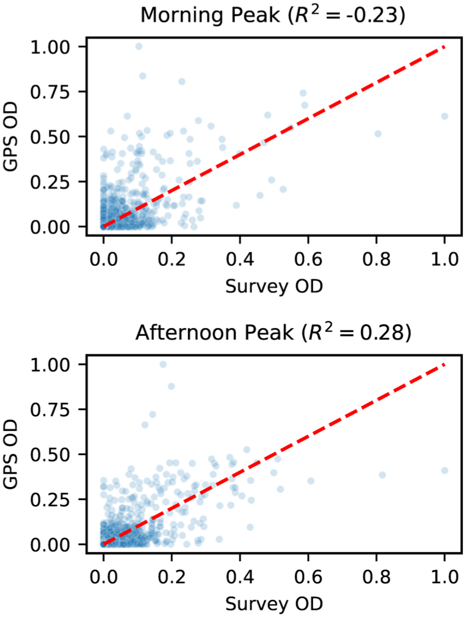As shown in Figure 1, The resulting $R^{2}$ values are extremely low (morning peak: $R^{2} = - 0.23$ , afternoon peak: $R^{2} = 0.28$ ), indicating that the two datasets do not exhibit a strong linear relationship in trip counts. The results suggest that magnitude alignment is not feasible through simple scaling or regression-based adjustments.

Figure 1.

Comparison of global positioning system (GPS) and survey origin–destination (OD) flow for morning (6–10 a.m.) (top) and afternoon (3–7 p.m.) (bottom) periods.

Despite the two datasets differing in scale, they may still exhibit similarity in their underlying spatial structure. To explore this, we compute the Spearman rank correlation between survey and GPS OD flows across five time-of-day periods, which compares the consistency of OD-flow rankings between the two datasets. As summarized in Table 1, the two data sources show strong spatial consistency during commute-dominated daytime periods (6 a.m.–7 p.m.), reflecting common spatial patterns of regular and predictable flows. Evening flows exhibit moderate correspondence ( $ρ = 0.50$ ), while late-night flows present weak spatial alignment ( $ρ = 0.20$ ). This is consistent with sparse survey sampling and more heterogeneous travel behavior.

Table 1.

Spatial Spearman Correlations between Survey-Based and GPS-Derived OD Flows across Time Periods

Time-of-day	Time range	Spearman $ρ$ *
AM peak	6–10 a.m.	0.62
Midday	11 a.m.–3 p.m.	0.60
PM peak	3–7 p.m.	0.61
Evening	8 p.m.–midnight	0.50
Midnight	Midnight–6 a.m.	0.20

Note: GPS = global positioning system; OD = origin–destination.

Following common interpretations, $| ρ | < 0.3$ indicates weak consistency, $0.3 \leq | ρ | < 0.5$ indicates moderate consistency, and $| ρ | \geq 0.5$ indicates strong consistency. Bold values indicate strong spatial consistency period. These criteria support comparison of spatial alignment across mobility segments.

To further examine the structural properties of these OD matrices, we compute the cumulative singular-value spectra of both datasets by singular value decomposition. The results are shown in Figure 2. Over 80% of the energy lies in the first few singular values, and this shows that both GPS and survey OD matrices are strongly low-rank, even with differences in sampling and temporal coverage. This low-rank behavior suggests that the OD matrices can be represented by a few dominant spatial and temporal latent patterns.

Figure 2.

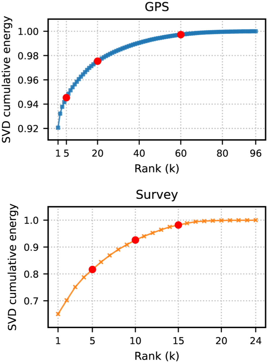
Cumulative singular value decomposition energy of the global positioning system (GPS) origin–destination (OD) matrix ( $2500 \times 96$ ) (top) and survey OD matrix ( $2500 \times 24$ ) (bottom).

Taken together, although the GPS and survey OD matrices differ considerably in magnitude, they exhibit a clear spatial correspondence during periods of regular travel demand. This suggests that the two data sources capture similar underlying patterns, while also reflecting source-specific biases. Moreover, the low-rank structure of the OD matrices motivates the use of a joint low-rank model to extract shared spatial patterns while accounting for source-specific temporal variations.

Methodology

To fuse the two heterogeneous data sources, we propose a dynamic joint latent factor model that decomposes each OD matrix into a shared spatial pattern matrix and a temporal pattern matrix. Our previous data analysis shows that the peak-period OD spatial patterns are highly consistent across both datasets, which supports the use of a shared spatial representation. For the temporal patterns, we model the latent temporal factors using a first-order linear dynamical system (LDS), since traffic demand is strongly influenced by its previous state ( 20 , 23 ). Overall, the proposed framework integrates low-rank factorization with state-space modeling, providing a compact and interpretable representation of high-dimensional OD flows ( 24 , 25 ).

Model Formulation

Shared Low-Rank Factorization

We denote the matrices $Y_{M} \in R^{L \times T_{M}}$ and $Y_{N} \in R^{L \times T_{N}}$ as the GPS-based and survey-based OD observations, where $L$ is the number of OD pairs and $T_{M}$ , $T_{N}$ are corresponding time horizons. For each OD dataset, we use a low-rank factorization that separates spatial structure from the temporal variation ( 24 ):

Y_{M} = W X_{M} + ε_{M}, Y_{N} = W X_{N} + ε_{N} .

(1)

where

$W \in R_{+}^{L \times K}$ = the shared spatial pattern matrix,

$X_{M} \in R^{K \times T_{M}}$ = the temporal pattern matrix for the GPS data,

$X_{N} \in R^{K \times T_{N}}$ = the temporal pattern matrix for the survey data,

$K$ = the number of latent mobility patterns ( $1 \leq K << \min (L, T_{M}, T_{N})$ ),

$ε_{M}$ = zero-mean Gaussian noise with covariance $R_{M}$ , and

$ε_{N}$ = zero-mean Gaussian noise with covariance $R_{N}$ .

This shared low-rank factorization model can also be regarded as an observation model in state-space model setting.

To obtain meaningful spatial patterns and balance the contributions of the two data sources, we first update $W$ by solving a weighted non-negative least squares (NNLS) problem ( 26 ):

\begin{matrix} W^{(init)} : = \arg \min_{W \geq 0} { \\ λ_{M} tr [{(Y_{M} - W X_{M})}^{⊤} R_{M}^{- 1} (Y_{M} - W X_{M})] \\ + λ_{N} tr [{(Y_{N} - W X_{N})}^{⊤} R_{N}^{- 1} (Y_{N} - W X_{N})]}, \end{matrix}

(2)

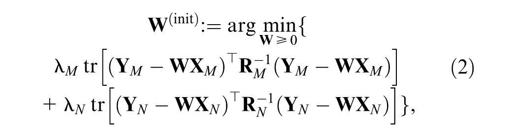
where

$λ_{M} + λ_{N} = 1$ .

The adaptive weights $λ_{M}$ and $λ_{N}$ are introduced because the two datasets differ in temporal coverage ( $T_{M} \neq T_{N}$ ). Without weighting, the dataset with more time points would dominate the reconstruction objective and bias the update of $W$ . The non-negativity constraint on $W$ improves interpretability by ensuring that each latent pattern contributes additively to each OD pair. This avoids mixed positive and negative loadings in the spatial basis, making the learned columns of $W$ easier to interpret as spatial intensity patterns.

Starting from the NNLS solution $W^{(init)}$ , we further refine $W$ to improve the stability and interpretability of the learned spatial patterns. Specifically, we consider the following regularized reconstruction objective with a soft orthogonality penalty:

\begin{matrix} \min_{W \geq 0} {L (W) + λ_{w} ∥ W^{⊤} W - diag (W^{⊤} W) ∥_{F}^{2}}, \end{matrix}

(3)

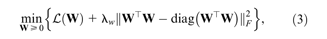
where

$L (W)$ = the weighted reconstruction loss defined above, and

$λ_{w} = 0.01$ .

This regularization improves the stability of the learned spatial pattern matrix across different random initializations, while preserving the reconstruction quality obtained from the NNLS initialization. Such stability is essential for interpretability: if different initializations yield substantially different estimates of $W$ , the resulting spatial patterns cannot be regarded as a reliable basis for interpretation.

Independent Temporal Dynamics

Let $x_{t}^{(M)} \in R^{K}$ and $x_{t}^{(N)} \in R^{K}$ denote the latent state at time $t$ for the two datasets. Vertically stacking these states over all time steps yields the temporal factor matrices $X_{M} = [x_{1}^{(M)}; \dots; x_{T_{M}}^{(M)}] \in R^{K \times T_{M}}$ and $X_{N} = [x_{1}^{(N)}; \dots; x_{T_{N}}^{(N)}] \in R^{K \times T_{N}}$ . To characterize how mobility activity evolves over time, we model each temporal latent process using a first-order LDS ( 24 ):

x_{t + 1}^{(M)} = F_{M} x_{t}^{(M)} + η_{t}^{(M)}, η_{t}^{(M)} ~ N (0, Q_{M}),

(4)

x_{t + 1}^{(N)} = F_{N} x_{t}^{(N)} + η_{t}^{(N)}, η_{t}^{(N)} ~ N (0, Q_{N}),

(5)

where

$F_{s} \in R^{K \times K}$ = the state-transition matrix that defines the linear update from one time step to the next, and

$Q_{s}$ = the process-noise covariance that captures temporal variability not explained by the deterministic transition, with $s \in {M, N}$ indexing the two datasets.

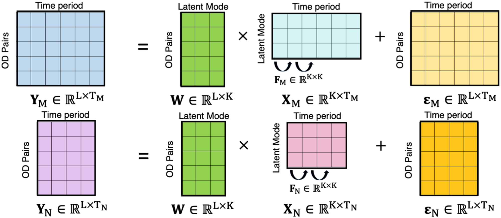
In summary, by combining Equations 1 and 3, the model allows the spatial pattern matrix $W$ to capture OD patterns that are consistently expressed in both datasets, while the separate temporal factors and noise terms account for source-specific sampling and behavioral differences over time. This structure enables the model to learn a unified spatial representation without imposing identical temporal dynamics across datasets. The overall latent factor representation is illustrated in Figure 3.

Figure 3.

Latent factor representation of the origin–destination (OD) matrices. Each dataset shares the spatial pattern matrix $W$ and has its own temporal factors ( $X_{M}$ for global positioning system (GPS), $X_{N}$ for survey).

Model Inference

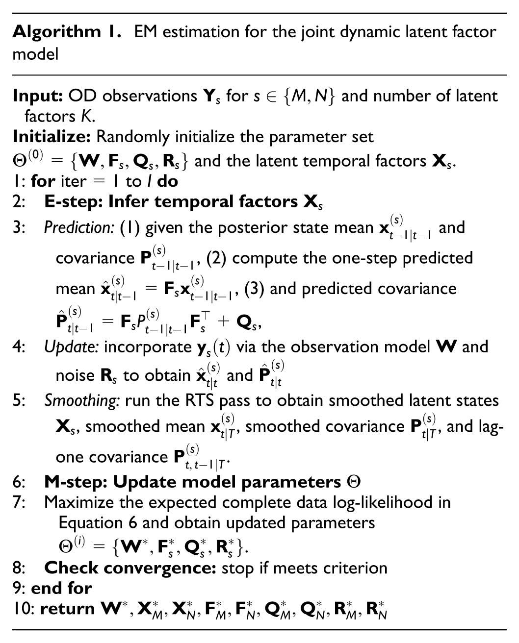
We estimate the model parameters using the expectation–maximization (EM) algorithm ( 24 , 25 , 27 ). The algorithm alternates between estimating the latent variables given the current parameters (E-step) and updating the parameters given the expected latent variables (M-step). In this study, we regard temporal latent matrices $X_{s}$ as latent variables, and other matrices, including the shared spatial latent matrix $W$ , as parameters, denoted by $Θ = {W, F_{s}, Q_{s}, R_{s}}, s \in {M, N}$ .

In the E-step, given the current parameter estimates $Θ^{(i)}$ at iteration $i$ , we compute the posterior means and covariances of the latent temporal factors for each dataset $p (X_{s} ∣ Y_{s}, Θ^{(i)})$ ( 24 ). Since the two state processes are conditionally independent given the parameters, two separate Rauch-Tung-Striebel (RTS) Kalman smoothers are employed. The smoother provides the sufficient statistics for the hidden states, namely the smoothed mean ${\hat{x}}_{t}^{(s)}$ (the estimated temporal factors $X_{s}$ ) and their covariances ( ${\hat{P}}_{t}^{(s)}$ , ${\hat{P}}_{t, t - 1}^{(s)}$ ).

In the M-step, we update the parameters by maximizing the complete-data log-likelihood with respect to $Θ$ ( 24 ):

\begin{matrix} \log p (Y, X ∣ Θ) = \sum_{s \in {M, N}} (L_{prior}^{(s)} (X_{s}) + L_{dyn}^{(s)} (X_{s}; F_{s}, Q_{s}) \\ + L_{obs}^{(s)} (Y_{s}, X_{s}; W, R_{s})), \end{matrix}

(6)

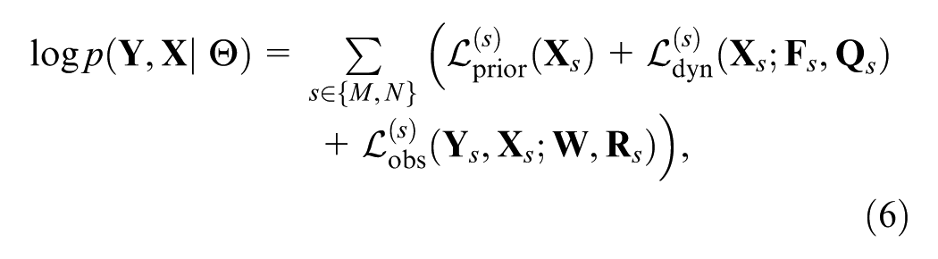
where

$L_{prior} (\cdot)$ = the initial-state prior,

$L_{dyn} (\cdot)$ = the temporal dynamics under the LDS, and

$L_{obs} (\cdot)$ = the observation model linking OD flows to latent factors.

The closed-form updates for $F_{s}$ , $Q_{s}$ , and $R_{s}$ follow the standard EM updates for LDS models based on the sufficient statistics obtained in the E-step ( 24 , 27 ). For the shared spatial pattern matrix $W$ , we first solve the weighted non-negative least squares problem described in Equation 2. Rather than fixing the modality weights a priori, we tune $λ_{M}$ using the Optuna hyperparameter optimization framework, which searches over $[0, 1]$ for the value that balance the reconstruction performance across both datasets ( 28 ). Starting from the resulting NNLS solution $W^{(init)}$ , we then perform the regularized refinement using 20 projected gradient steps in Equation 3. At each step, $W$ is updated along the negative gradient direction of the penalized objective, projected onto the nonnegative orthant, and accepted only if the objective decreases. A backtracking strategy is used to adaptively shrink the step size, starting from 0.01 and halving it when necessary.

With the updates for $W$ , $F_{s}$ , $Q_{s}$ , and $R_{s}$ , the M-step is fully specified. The complete EM algorithm is summarized in Algorithm 1. All parameters and latent temporal factors are initialized with small random values. The algorithm iteratively performs the E-step and M-step until the change in the $\log p (Y, X ∣ Θ)$ less than $10^{- 4}$ . As shown in Figure 4, the log-likelihood $\log p (Y, X ∣ Θ)$ decreases rapidly and at 72 iterations the change between successive iterations falls below the convergence threshold. The number of latent patterns was fixed at $K = 5$ in this study, since both matrices exhibit a clear low-rank structure with most of their energy concentrated in the leading components. As shown in Figure 2, the first five components explain more than 80% of the total energy in the GPS matrix and 94% in the survey matrix.

Algorithm 1.

EM estimation for the joint dynamic latent factor model

Input: OD observations

Y_{s}

for

s \in {M, N}

and number of latent factors

K

.
Initialize: Randomly initialize the parameter set

Θ^{(0)} = {W, F_{s}, Q_{s}, R_{s}}

and the latent temporal factors

X_{s}

.
1: for

iter = 1

I

do
2: E-step: Infer temporal factors

X_{s}

3: Prediction: (1) given the posterior state mean

x_{t - 1 | t - 1}^{(s)}

and covariance

P_{t - 1 | t - 1}^{(s)}

, (2) compute the one-step predicted mean

{\hat{x}}_{t | t - 1}^{(s)} = F_{s} x_{t - 1 | t - 1}^{(s)}

, (3) and predicted covariance

{\hat{P}}_{t | t - 1}^{(s)} = F_{s} P_{t - 1 | t - 1}^{(s)} F_{s}^{⊤} + Q_{s}

,
4: Update: incorporate

y_{s} (t)

via the observation model

W

and noise

R_{s}

to obtain

{\hat{x}}_{t | t}^{(s)}

and

{\hat{P}}_{t | t}^{(s)}

5: Smoothing: run the RTS pass to obtain smoothed latent states

X_{s}

, smoothed mean

x_{t | T}^{(s)}

, smoothed covariance

P_{t | T}^{(s)}

, and lag-one covariance

P_{t, t - 1 | T}^{(s)}

.
6: M-step: Update model parameters

Θ

7: Maximize the expected complete data log-likelihood in Equation 6 and obtain updated parameters

Θ^{(i)} = {W^{*}, F_{s}^{*}, Q_{s}^{*}, R_{s}^{*}}

.
8: Check convergence: stop if meets criterion
9: end for
10: return

W^{*}, X_{M}^{*}, X_{N}^{*}, F_{M}^{*}, F_{N}^{*}, Q_{M}^{*}, Q_{N}^{*}, R_{M}^{*}, R_{N}^{*}

Figure 4.

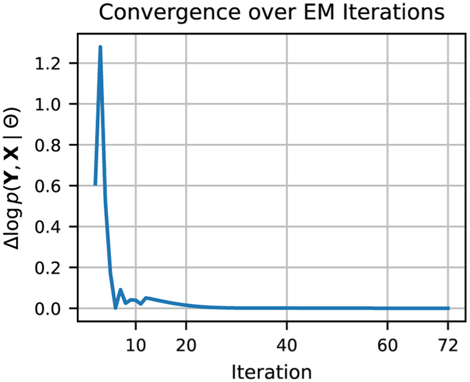
Convergence of the expectation–maximization (EM) algorithm measured by the change in the Q-function ( $dQ$ ).

Results

Model Performance

The proposed joint latent factor model achieves high reconstruction accuracy for both datasets. Figure 5 shows the model’s ability to reconstruct observed OD flows from latent matrices, measured by $R^{2}$ . The reconstructed OD values align closely with the 45-degree line for both datasets, resulting in $R^{2} = 0.84$ for GPS and $R^{2} = 0.78$ for the survey. While the model achieves good overall fit, few high-volume OD pairs exhibit larger dispersion and systematic deviations from the diagonal. Such behavior is consistent with the heavy-tailed nature of OD flow distributions, where extreme values are known to be challenging to reconstruct accurately ( 29 ). Additionally, specifically in the survey dataset, a subset of points aligns with the horizontal axis (observed $> 0$ , reconstructed $\approx 0$ ). This reflects the model’s capacity to filter sampling artifacts: isolated trips derived from expansion weights, which lack corroborating spatiotemporal structure, are treated as noise and suppressed. This effectively isolates the robust mobility backbone from random sampling fluctuations. The alignment indicates that the shared spatial factors and independent temporal factors recover meaningful structure in travel demand rather than simply smoothing noise. These results provide a reliable foundation for interpreting the latent patterns in the following sections.

Figure 5.

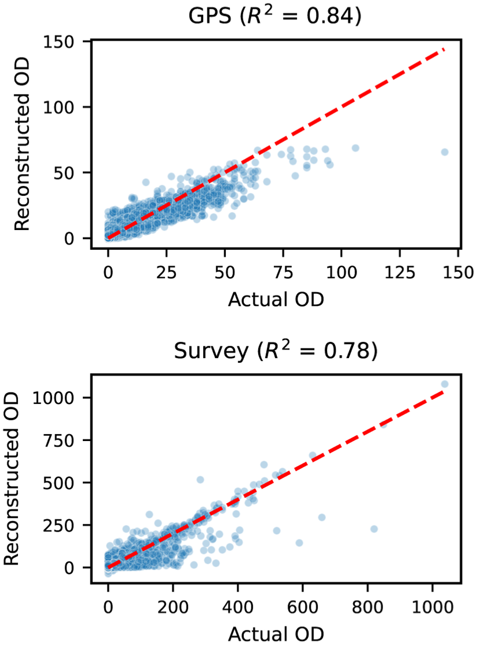
Reconstructed versus actual origin–destination (OD) flows for global positioning system (GPS) (top) and survey (bottom).

Temporal Latent Patterns

To understand the hourly evolution of travel demand in both datasets, we examine the temporal latent patterns matrices $X_{M}$ (GPS) and $X_{N}$ (survey). Each row of the temporal latent matrices corresponds to one of the latent mobility patterns. Because the shared spatial matrix $W$ is constrained to be nonnegative, the signs of $X_{M}$ and $X_{N}$ indicate whether a temporal factor amplifies or suppresses its associated spatial pattern at a given hour.

Figure 6 presents the five temporal patterns: the top panel shows GPS factors across 96-hours (four weekdays), and the bottom panel shows the 24-hour weekday profile from the survey. Across both datasets, the dominant factors exhibit clear morning (6–10 a.m.) and afternoon (3–7 p.m.) activity peaks, aligning with well-known commuting patterns. An important structural feature is the contrast between positive and negative magnitudes: positive values indicate hours when a latent pattern contributes more strongly to OD flows, whereas negative values reflect periods when that pattern is relatively suppressed. Furthermore, several patterns display contrasting magnitudes between the morning and afternoon periods in both datasets, suggesting that each pattern captures a different phase of the daily mobility cycle.

Figure 6.

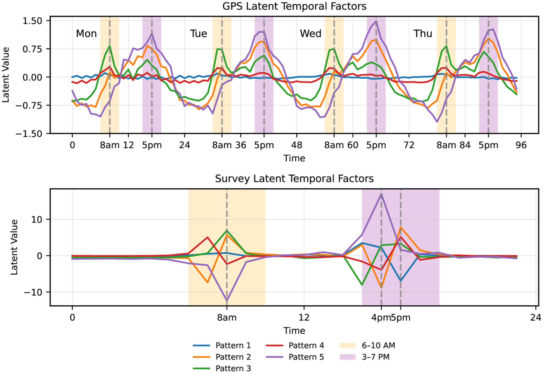
Latent temporal factors learned from global positioning system (GPS) ( $X_{M}$ ) data (top) and survey ( $X_{N}$ ) data (bottom).

A closer comparison at the pattern level reveals clear differences in which latent patterns dominate each peak period. For example, during the morning peak, the GPS data are driven almost entirely by Pattern 3, which reaches the strongest magnitude around 8 a.m., while the other factors show only moderate increases. In contrast, the survey data display a more distributed structure: Patterns 2, 3, and 4 all exhibit positive magnitudes at 8 a.m., indicating that the survey-derived morning peak is jointly supported by multiple factors rather than a single dominant one. The afternoon peak shows greater agreement between the two sources (Patterns 2, 3, and 5). During the afternoon peaking period, Pattern 5 provides the strongly positive magnitude during the 4–6 p.m. time period across both datasets, with Pattern 2 contributing as a secondary component. Thus, while the two datasets share similar timing of peak demand, they differ in how individual latent patterns compose those peaks, particularly in the morning.

Overall, these temporal factors summarize the common daily rhythm of urban travel demand and highlight source-specific differences in smoothness and amplitude. Building on these insights, the next section turns to the spatial dimension to examine how the most influential latent patterns manifest across geographic areas and land-use contexts, where the joint interpretation of $W$ and $(X_{M}, X_{N})$ becomes more informative.

Shared Spatial OD Patterns

In this section, we first analyze the spatial latent pattern matrix $W$ , which represents the main OD connectivity patterns shared by both data sources. We then relate these patterns to the functional characteristics of different urban zones to examine how dominant OD clusters correspond to zones with high outflows (origins) and inflows (destinations) across the city.

Latent Spatial Structure

The spatial matrix $W$ indicates how strongly each OD pair contributes to each latent pattern, providing a data-driven decomposition of the city’s underlying mobility structure. Since $W$ is shared across the GPS and survey datasets, each of its columns represents a latent spatial pattern that is common to both sources. The values within a column vary across OD pairs: larger values indicate OD pairs that contribute more strongly to the corresponding latent pattern and, therefore, define its dominant spatial structure. To examine spatial homogeneity and heterogeneity across the city, we cluster the 2,500 OD pairs using K-means and evaluate each cluster’s average contribution to each pattern based on its $W$ values. Formally, the contribution of cluster $c$ to pattern $k$ is computed as:

{AvgContribution}_{c, k} = \frac{1}{| {Cluster}_{c} |} \sum_{l \in {Cluster}_{c}} W_{l, k} .

(7)

To ensure comparability across clusters within each mode, these values are normalized into relative shares:

{Share}_{c, k} = \frac{{AvgContribution}_{c, k}}{\sum_{c^{'}} {AvgContribution}_{c^{'}, k}} .

(8)

Table 2 reports the contributions by cluster, along with entropy and Gini indices. A full scatterplot of OD-pair magnitudes by cluster and pattern is provided in the Appendix for reference. The results indicate a strong dominance of Cluster 1 and Cluster 2, which together account for more than 50% of total magnitude in each pattern, while smaller clusters contribute diminishing shares. The moderate entropy values (2.5–2.6) and Gini coefficients (0.40–0.43) suggest that each latent pattern is concentrated in a few leading clusters, with the remaining clusters contributing only marginally. This suggests that the patterns are structured around a few dominant spatial clusters OD pairs, rather than being either tightly localized or uniformly dispersed.

Table 2.

Cluster Dominance (% of Mean Magnitude) by Latent Pattern, Entropy, and Gini Index

Pattern	1	2	3	4	5
Cluster 1	27.78	29.04	29.16	28.40	25.78
Cluster 2	22.38	23.57	23.20	22.19	22.35
Cluster 3	18.13	16.99	17.10	17.58	18.89
Cluster 4	13.68	13.34	12.95	13.34	15.34
Cluster 5	9.65	9.36	9.34	9.78	10.20
Other	$< 9$	$< 9$	$9$	$< 9$	$< 9$
Entropy*	2.547	2.512	2.522	2.543	2.546
Gini*	0.417	0.435	0.431	0.419	0.408

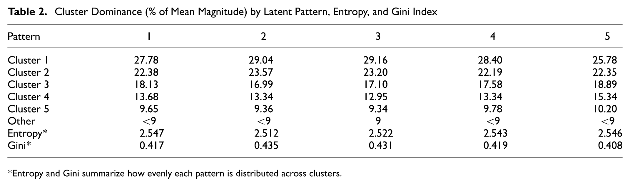
Entropy and Gini summarize how evenly each pattern is distributed across clusters.

Although latent patterns are identified through clustering of OD pairs, trip activity is inherently expressed at the zone level through the origins’ and destinations’ characteristics. Therefore, to examine how these patterns relate to population and land-use characteristics, we aggregate OD flows by origin and destination and analyze zone-level outflows (origin totals) and inflows (destination totals) at the zone level. Figure 7 illustrates the spatial distribution of sending (origin-dominant) and receiving (destination-dominant) zones for Cluster 1, which is most strongly associated with all latent patterns. Across patterns, the maps reveal a clear outer-to-inner structure. Inflow-dominant zones (blue) are concentrated in downtown and south area (i.e., hospital, residential), whereas outflow-dominant zones (yellow) are located mainly in residential and rural fringe areas. Mixed zones (green) appear in several inner-urban neighborhoods and reflect their dual residential and employment functions. Although each pattern highlights different combinations of residential and peripheral areas, they all reflect variations of the same fundamental spatial logic: trips predominantly originate from the outskirts and converge toward central activity hubs.

Figure 7.

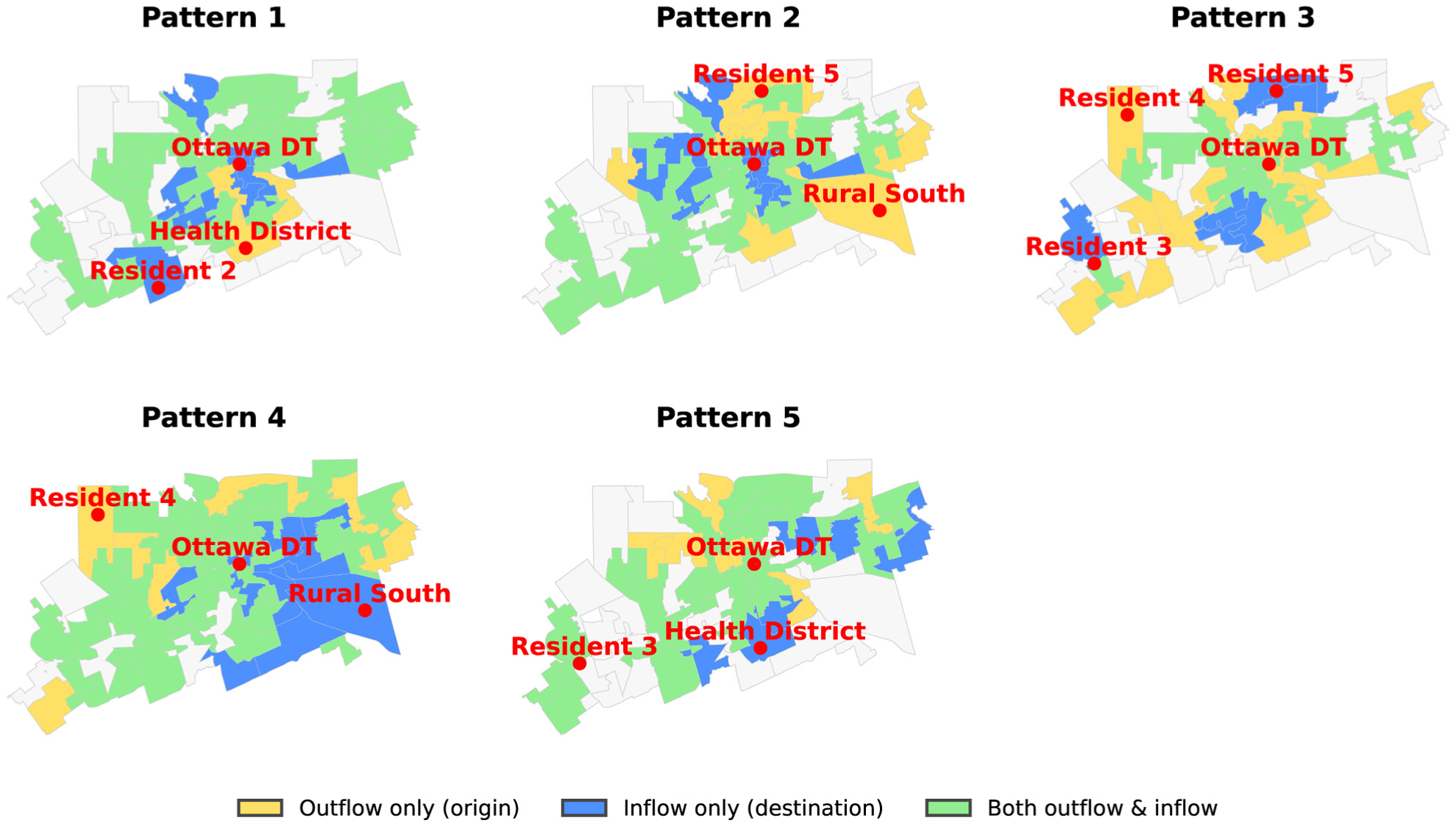
Zone-level (origins) and inflows (destinations) for Cluster 1 across five latent patterns.

Socio-Demographic Analysis

To further interpret the origin (outflow) and destination (inflow) roles implied by the latent patterns, we link them to zone-level socio-demographic profiles. We estimate separate ordinary least squares regressions following standard linear modeling practice ( 30 ). The models are implemented in Python using the scikit-learn library and are fitted separately for outflow and inflow totals in the highest-contributing OD pairs (Clusters 1–3) of each pattern. Table 3 shows that the explanatory variables cover demographic composition, household income, employment characteristics, and household size at both origins and destinations, all of which are commonly linked to commute intensity in urban travel behavior. We retain all coefficients and highlight significant estimates in the table, allowing us to identify the dominant variables associated with the spatial footprint of each latent pattern.

Table 3.

Operational Definitions of Explanatory Variables Used in the Ottawa Case Study

Category	Definition	Variable
Demographic	Youth population (15–24 years old)	Youth pop
	Adult population (25–44 years old)	Adult pop
	Middle-aged population (45–64 years old)	Middle-aged pop
Household size	Households with 2 persons	HH size 2
	Households with 3 persons	HH size 3
	Households with 4–5 persons	HH size 4–5
Employment type	Public office employment	Public office jobs
Employment type	Private office employment	Private office jobs

Note: HH = household.

Morning-Peaking Patterns

In the morning period, we focus on Patterns 2 and 3, which show clear morning (AM) contribution in the temporal factors (Figure 6). Figure 8 visualizes these significant coefficients for both survey- and GPS-based OD matrices (survey in blue, GPS in orange), enabling a direct comparison of how the two data sources characterize the outflow and inflow drivers of AM travel patterns. To emphasize the dominant factors of morning travel, our discussion focuses on statistically significant variables, which are shown with darker bars, while non-significant coefficients are displayed with lighter shading for completeness.

Figure 8.

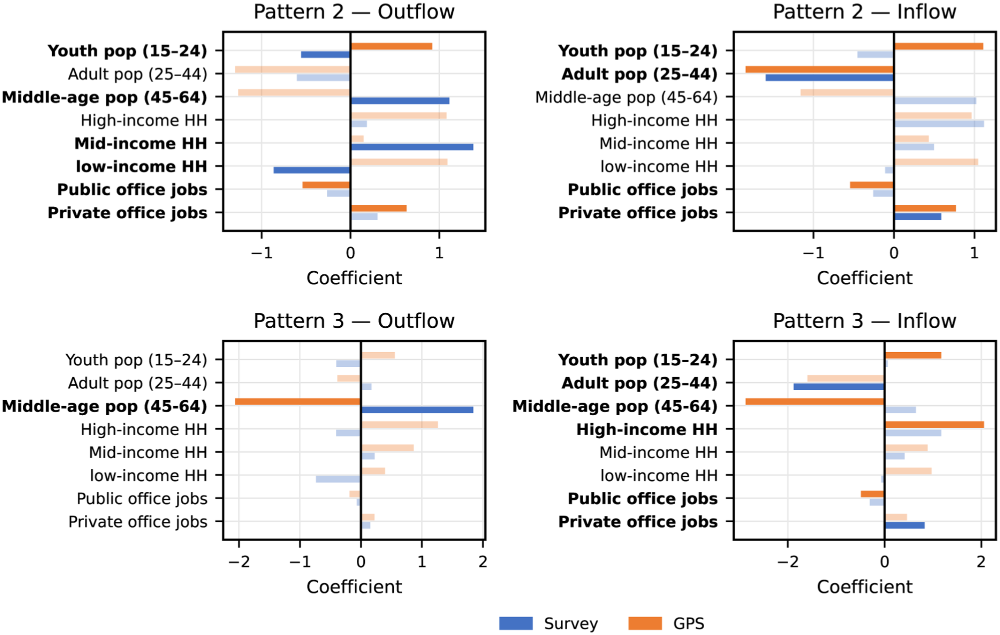
Outflow and inflow by latent pattern during the AM peak. The top-left panel shows Pattern 2 outflow, the top-right panel shows Pattern 2 inflow, the bottom-left panel shows Pattern 3 outflow, and the bottom-right panel shows Pattern 3 inflow. Survey-based coefficients are shown in blue, and GPS-based coefficients are shown in orange.

We first examine Pattern 2, which captures office-oriented morning commuting flows. On the outflow side, the GPS-based model shows stronger associations with younger populations and areas linked to private-office activity, whereas the survey-based model emphasizes middle-aged and mid-income households as the main contributors. This contrast suggests that GPS data are more sensitive to younger commuters working in private-office environments, while the survey better represents middle-aged and mid-income groups that are less prevalent in passive mobile data. On the inflow side, both datasets consistently identify private-office employment as the dominant correlate of morning inflows, while adult population shares are negatively associated with inflows. The GPS results additionally indicate stronger inflows toward youth-dominated zones and weaker associations with public-office areas, extending the demographic contrast observed on the outflow side.

Pattern 3 exhibits weaker and less consistent associations across the two datasets, indicating a more heterogeneous morning travel pattern. On the outflow side, both models emphasize the middle-aged population but with opposite signs: the survey associates middle-aged residents with higher outflows, whereas the GPS model shows a strong negative association. On the inflow side, the GPS-based results reveal a sharper demographic contrast, with positive effects for youth and high-income households and negative effects for middle-aged residents and public-office employment. In contrast, the survey model displays more muted relationships, with only modest demographic effects and a weak association with private-office jobs. Together, these discrepancies suggest that Pattern 3 captures a less stable or more behaviorally diverse form of morning travel that is represented differently by survey and GPS data.

Afternoon-Peaking Patterns

The afternoon analysis examines Patterns 2, 3, and 5, which are the modes with the strongest PM activity in the temporal profiles (Figure 6). As in the morning analysis, we estimate outflow- and inflow-side regressions for each pattern to identify the socio-demographic variables most strongly associated with their OD flows. The corresponding outflow and inflow coefficients for the afternoon patterns are reported in Figure 9.

Figure 9.

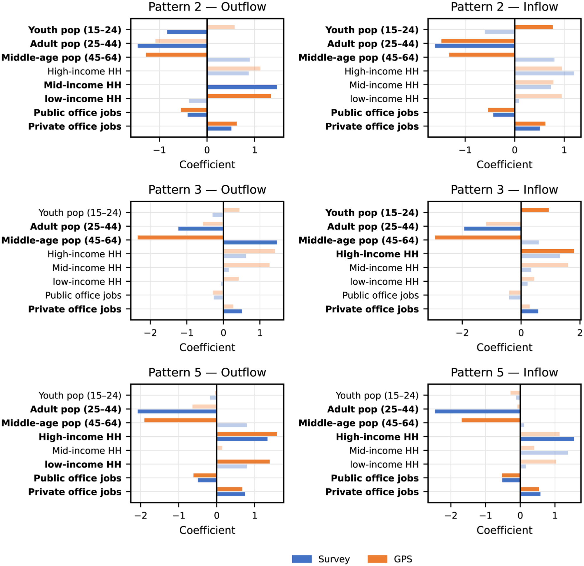
Outflow and inflow by latent pattern during the PM peak. The top-left panel shows Pattern 2 outflow, the top-right panel shows Pattern 2 inflow, the middle-left panel shows Pattern 3 outflow, the middle-right panel shows Pattern 3 inflow, the bottom-left panel shows Pattern 5 outflow, and the bottom-right panel shows Pattern 5 inflow. Survey-based coefficients are shown in blue, and GPS-based coefficients are shown in orange.

Pattern 2 reflects the dominant PM return flow from private-office districts. Both datasets show a consistent employment structure, with private-office areas attracting these flows and public-office areas contributing negatively on both the outflow and inflow sides. The key differences still arise in the socio-demographic signals: GPS associates this pattern with younger and lower-income residents, whereas the survey links it to middle-income, adult households. These contrasts indicate that the two datasets capture different commuter groups participating in the same office-oriented PM return movement. Pattern 3 shows the clearest split between the two datasets. The survey maintains an employment-related return flow with positive contributions from private-office areas and middle-aged populations. In contrast, GPS shows no job-related effects on the outflow side and instead exhibits strong inflows toward youth and high-income zones. This indicates that GPS captures a selective subgroup of younger, higher-income travelers rather than the broader worker flows reflected in the survey.

Pattern 5 represents the second major PM structure and the most income-differentiated mode. Both datasets show a consistent outflow profile: high-income households and private-office employment contribute positively, while public-office areas contribute negatively. On the inflow side, the survey highlights strong pull from high-income and private-office zones, whereas GPS again shows pronounced negative responses for middle-aged populations. Overall, both datasets depict an affluent PM flow connecting higher-income residential areas with office-dominated destinations.

Discussion and Conclusion

This study develops a dynamic joint latent factor model to fuse GPS- and survey-based OD matrices. The model learns a shared spatial structure and separate temporal dynamics for each source. The shared loading matrix reveals consistent OD patterns, while the temporal factors show how these patterns evolve over time. Because surveys provide infrequent behavioral baselines and GPS offers continuous temporal coverage, the framework enables long-term comparison of mobility patterns and systematic monitoring of how OD flows change across years. The method also allows a direct behavioral comparison between vehicle-trace data and self-reported car trips, quantifying where the two sources converge or diverge. However, this analysis is currently restricted to motorized vehicle flows to maintain structural comparability between the datasets. Future work could leverage the framework’s extensibility to incorporate non-motorized modes, providing a more holistic view of multi-modal urban mobility.

With regard to computational scalability, while this study focuses on a mid-sized metropolitan area, the proposed framework is designed to scale to larger regions with hundreds of thousands of OD pairs. Theoretically, the low-rank factorization reduces the effective degrees of freedom from $L \times T$ to $(L + T) \times K$ , meaning the computational cost grows linearly with the number of OD pairs ( $L$ ) rather than quadratically. Practically, for massive datasets, the sparsity of OD matrices can be leveraged using sparse matrix operations, which compute gradients only on non-zero entries ( 26 ). Furthermore, spatial aggregation (as demonstrated with the 50-district design) or hierarchical decomposition strategies can be employed to manage dimensionality without sacrificing the extraction of macro-level mobility structures.

In the following section, we provide a detailed interpretation of the temporal negative magnitudes and spatial patterns, concluding with a discussion on the implications for urban mobility planning.

Temporal Negative Magnitude Analysis

In the temporal factors $X_{M}$ and $X_{N}$ , some components take negative values, particularly in Patterns 2, 3, and 5 during late-night and early-morning hours, as shown in Figure 6. This behavior arises naturally from the proposed factorization. The OD matrix is represented as $WX$ , where the spatial factor $W$ is constrained to be non-negative while the temporal factors are unconstrained. Under this formulation, negative values in $X$ correspond to periods in which the contribution of a latent pattern is suppressed relative to its baseline level, allowing the model to represent very low or near-zero OD activity without forcing all temporal components to remain positive.

Consequently, this unconstrained temporal structure leads to a subset of reconstructed OD entries taking negative values, as illustrated in Figure 10. These entries account for 18.53% of the GPS-based and 24.32% of the survey-based reconstruction. However, unlike the structural interpretation of negative temporal factors, these reconstructed negatives represent negligible numerical artifacts rather than model instability. Crucially, as the distributions in Figure 10 show, these values are heavily concentrated around zero, and 99% correspond to OD pairs with zero observed flows. This indicates they arise primarily from smoothing effects in sparse regions. While the survey reconstruction exhibits a larger range of negative values, this reflects the high variance and heavy-tailed distribution of survey expansion weights, relative to the total expanded volume of active trips, these fluctuations remain minor. Thus, simple non-negativity clipping is sufficient to ensure valid demand estimates without compromising the model’s accuracy.

Figure 10.

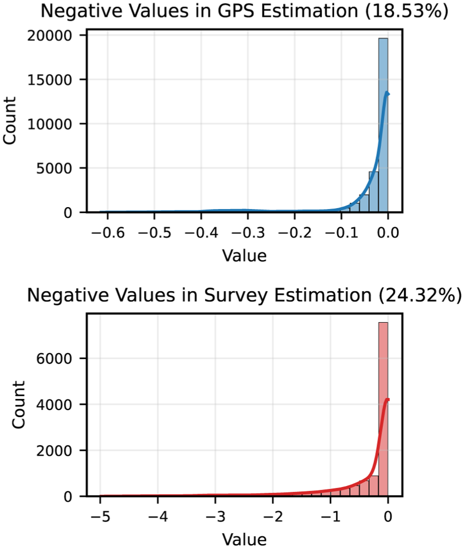
Distribution of negative origin–destination estimates for global positioning system (GPS) data (top) and survey data (bottom).

Spatial Patterns Analysis

Building on the temporal results, the spatial patterns reveal how the latent modes manifest across different parts of the urban region. The morning latent patterns reveal a stable and coherent commuting structure shaped by fixed work schedules and the spatial concentration of employment. Both datasets align closely in identifying the same office-oriented flows, which indicates that morning travel is governed primarily by structural constraints rather than behavioral variation. The differences between GPS and survey signals arise largely from their sampling mechanisms. GPS over-represents groups with higher mobility resources, such as younger and higher-income drivers, whereas the survey reflects a more complete cross-section of the resident workforce. These contrasts therefore reflect differences in population representation rather than differences in the underlying mobility behavior.

The afternoon patterns display greater divergence because afternoon travel is less constrained and more behaviorally heterogeneous. As work schedules loosen and discretionary activities increase, mobility becomes more fragmented across population groups. The GPS data capture this flexibility more sharply, highlighting younger and higher-income travelers whose activity patterns are less regular and more resource-dependent. The survey exhibits smoother gradients and maintains clearer associations with the broader workforce. Patterns 3 and 5 illustrate this dynamic most clearly: GPS responds strongly to youth and high-income zones while showing weaker employment-related effects, whereas the survey continues to reflect flows anchored in office locations and middle-aged workers. These differences show that afternoon modes capture multiple behavioral sub-regimes rather than a single unified flow.

Taken together, the latent patterns reveal that GPS and survey data provide complementary perspectives on urban mobility. GPS captures the flexible and high-intensity component of car travel, while the survey reflects the structural backbone of routine commuting. The joint factor model clarifies when discrepancies arise from sampling bias and when they represent genuine behavioral variation across time periods and traveler groups. These findings emphasize that OD matrix fusion must account for differences across latent mobility regimes.

Implications

From a practical standpoint, these findings offer several implications for mobility planning. The shared spatial factors provide a stable representation of the city’s underlying OD structure, which changes only gradually over time. This stability allows planners to use survey-informed spatial patterns as a behavioral baseline and to track medium- and long-term demand evolution by combining them with continuously collected GPS data. In data-scarce environments where surveys are available only every few years, this approach enables year-to-year and even day-to-day monitoring of travel patterns.

Recognizing the complementary strengths of the two data sources also supports better-informed OD modeling. Survey data provide a reliable basis for representing routine morning commuting, while GPS better captures the flexible and heterogeneous flows that dominate afternoon and discretionary travel. Finally, the interpretability of the latent modes allows planners to link OD patterns to socio-demographic and land-use conditions, enabling targeted corridor planning, demand management, and equity assessments. By integrating these insights, planners can develop OD models that reflect both stable structural patterns and the behavioral diversity present in contemporary urban mobility.

Supplemental Material

sj-pdf-1-trr-10.1177_03611981261444335 – Supplemental material for Joint Latent Analysis of Behavioral Patterns in Multi-Source Origin–Destination Matrices

Supplemental material, sj-pdf-1-trr-10.1177_03611981261444335 for Joint Latent Analysis of Behavioral Patterns in Multi-Source Origin–Destination Matrices by Xiting Zhang, Xudong Wang, Yubo Jiao, Lijun Sun and Luis Miranda-Moreno in Transportation Research Record

Footnotes

Acknowledgements

The authors thank SMATS Traffic Solutions for providing the aggregated GPS data and the City of Ottawa for providing the Household Travel Survey datasets.

Author Contributions

The authors confirm contribution to the paper as follows: study conception and design: X. Zhang, L. Sun, L. Miranda-Moreno; data collection: X. Zhang; analysis and interpretation of results: X. Zhang, X. Wang, Y. Jiao; draft manuscript preparation: X. Zhang, X. Wang. All authors reviewed the results and approved the final version of the manuscript.

Declaration of Conflicting Interests

The authors declared no potential conflicts of interest with respect to the research, authorship, and/or publication of this article.

Funding

The authors disclosed receipt of the following financial support for the research, authorship, and/or publication of this article: This project was made possible through financial support from the Government of Canada and the Fonds de recherche du Québec – Nature et technologies (FQNRT). Specifically, funding from the Government of Canada’s Environmental Damages Fund was provided under its Climate Action and Awareness Fund, while FRQNT contributed through the Programme de recherche en partenariat – Réduction des GES – Mobilité Durable.

ORCID iDs

Xiting Zhang

Xudong Wang

Yubo Jiao

Lijun Sun

Supplemental Material

Supplemental material for this article is available online.

References

Graells-Garrido

Opitz

Rowe

Arriagada

A Data Fusion Approach with Mobile Phone Data for Updating Travel Survey-Based Mode Split Estimates. Transportation Research Part C: Emerging Technologies, Vol. 155, 2023, p. 104285.

Rojas

M. B.

Sadeghvaziri

IV, E.

Jin

Comprehensive Review of Travel Behavior and Mobility Pattern Studies That Used Mobile Phone Data. Transportation Research Record: Journal of the Transportation Research Board, 2016. 2563: 71–79.

Zhao

Al-Khasawneh

M. B.

Tuoto

Cirillo

Data Fusion for Travel Analysis: Linking Travel Survey and Mobile Device Location Data. Transportation, 2025. https://doi.org/10.1007/s11116-025-10666-x

Egu

Bonnel

How Comparable Are Origin-Destination Matrices Estimated from automatic fare collection, origin-destination surveys and household travel survey? An empirical investigation in Lyon. Transportation Research Part A: Policy and Practice, Vol. 138, 2020, pp. 267–282.

Abrahamsson

Estimation of Origin-Destination Matrices Using Traffic Counts - A Literature Survey. IIASA Interim Report IR-98-021. International Institute for Applied Systems Analysis, Laxenburg, Austria, 1998.

Bera

Krishna Rao

K. V.

Estimation of Origin-Destination Matrix from Traffic Counts: The State of the Art. European Transport, Vol. 49, 2011, pp. 2–23.

Sun

Big Data-Driven Based Real-Time Traffic Flow State Identification and Prediction. Discrete Dynamics in Nature and Society, Vol. 2015, 2015, p. 284906.

Wang

Hou

Barth

Data-Driven Multi-Step Demand Prediction for Ride-Hailing Services Using Convolutional Neural Network. In Advances in Computer Vision: Proceedings of the 2019 Computer Vision Conference (CVC), (K. Arai and S. Kapoor eds.), Springer, Cham, Switzerland, Vol. 2, 2020, pp. 11–22.

Toole

J. L.

Colak

Sturt

Alexander

L. P.

Evsukoff

González

M. C.

The Path Most Traveled: Travel Demand Estimation Using Big Data Resources. Transportation Research Part C: Emerging Technologies, Vol. 58, 2015, pp. 162–177.

10.

Banús

D. P.

Mobility Demand Estimation: Understanding Data Collection Methodologies. Master’s thesis. Universitat Politècnica de Catalunya, Barcelona, Spain, 2023.

11.

Behara

K. N. S.

Bhaskar

Chung

A Novel Approach for the Structural Comparison of Origin-Destination Matrices: Levenshtein Distance. Transportation Research Part C: Emerging Technologies, Vol. 111, 2020, pp. 513–530.

12.

Bwambale

Choudhury

C. F.

Hess

Iqbal

M. S.

Getting the Best of Both Worlds: A Framework for Combining Disaggregate Travel Survey Data and Aggregate Mobile Phone Data for Trip Generation Modelling. Transportation, Vol. 48, No. 5, 2021, pp. 2287–2314.

13.

Jing

Zhang

Guo

Jiang

Context-Aware Matrix Factorization for the Identification of Urban Functional Regions with POI and taxi OD data. ISPRS International Journal of Geo-Information, Vol. 11, No. 6, 2022, p. 351.

14.

Cheng

Trepanier

Sun

Real-Time Forecasting of Metro Origin-Destination Matrices with High-Order Weighted Dynamic Mode Decomposition. Transportation Science, Vol. 56, No. 4, 2022, pp. 904–918.

15.

Zhou

Liu

Cui

Xiong

Transit Pattern Detection Using Tensor Factorization. INFORMS Journal on Computing, Vol. 31, No. 2, 2019, pp. 193–206.

16.

Sun

Sharpnack

Fan

Understanding Origin-Destination Ride Demand with Interpretable and Scalable Nonnegative Tensor Decomposition. Transportation Science, Vol. 57, No. 6, 2023, pp. 1473–1495.

17.

Sun

Axhausen

K. W.

Understanding Urban Mobility Patterns with a Probabilistic Tensor Factorization Framework. Transportation Research Part B: Methodological, Vol. 91, 2016, pp. 511–524.

18.

Wang

Fagette

Sartelet

Sun

A Probabilistic Tensor Factorization Approach to Detect Anomalies in Spatiotemporal Traffic Activities. Proc., IEEE Intelligent Transportation Systems Conference, Auckland, New Zealand, IEEE, New York, 2019, pp. 1658–1663.

19.

Xiao

Zhang

Goh

R. S. M.

Traffic Pattern Mining and Forecasting Technologies in Maritime Traffic Service Networks: A Comprehensive Survey. IEEE Transactions on Intelligent Transportation Systems, Vol. 21, No. 5, 2019, pp. 1796–1825.

20.

Wang

Sun

Diagnosing Spatiotemporal Traffic Anomalies with Low-Rank Tensor Autoregression. IEEE Transactions on Intelligent Transportation Systems, Vol. 22, No. 12, 2021, pp. 7904–7913.

21.

Smats Traffic Solutions Inc. Smart Traffic Monitoring and Origin–Destination Analysis Using Smats Bluemac Sensors. Technical Report. SMATS Traffic Solutions Inc., Ottawa, Canada, 2021.

22.

City of Ottawa and Ville de Gatineau. Ottawa–Gatineau Origin–Destination Household Travel Survey 2022: Technical Documentation and Data Summary. Technical Report. City of Ottawa and Ville de Gatineau, Ottawa, Canada, 2023.

23.

Wang

Sun

Anti-Circulant Dynamic Mode Decomposition with Sparsity-Promoting for Highway Traffic Dynamics Analysis. Transportation Research Part C: Emerging Technologies, Vol. 153, 2023, p. 104178.

24.

Shumway

R. H.

Stoffer

D. S.

An Approach to Time Series Smoothing and Forecasting Using the EM Algorithm. Journal of Time Series Analysis, Vol. 3, No. 4, 1982, pp. 253–264.

25.

Umatani

Imai

Kawamoto

Kunimasa

Time Series Clustering with an EM Algorithm for Mixtures of Linear Gaussian State Space Models. Pattern Recognition, Vol. 138, 2023, p. 109375.

26.

Kim

Park

Nonnegative Matrix Factorization Based on Alternating Nonnegativity Constrained Least Squares and Active Set Method. SIAM Journal on Matrix Analysis and Applications, Vol. 30, No. 2, 2008, pp. 713–730.

27.

Ghahramani

Hinton

G. E.

Parameter Estimation for Linear Dynamical Systems. Technical Report CRG-TR-96-2. University of Toronto, Ontario, Canada, 1996.

28.

Akiba

Sano

Yanase

Ohta

Koyama

Optuna: A Next-Generation Hyperparameter Optimization Framework. Proc., 25th ACM SIGKDD International Conference on Knowledge Discovery & Data Mining, Anchorage, AK, Association for Computing Machinery, New York, 2019, pp. 2623–2631.

29.

Hazelton

M. L.

Inference for Origin–Destination Matrices: Estimation, Prediction and Reconstruction. Transportation Research Part B: Methodological, Vol. 35, No. 7, 2001, pp. 667–676.

30.

Wooldridge

J. M.

Introductory Econometrics: A Modern Approach. 6th ed. Cengage Learning, Boston, MA, 2015.

Supplementary Material

Please find the following supplemental material available below.

For Open Access articles published under a Creative Commons License, all supplemental material carries the same license as the article it is associated with.

For non-Open Access articles published, all supplemental material carries a non-exclusive license, and permission requests for re-use of supplemental material or any part of supplemental material shall be sent directly to the copyright owner as specified in the copyright notice associated with the article.

0.16 MB

0.00 MB