
Abstract
This research provides a comparative assessment of data imputation techniques for item nonresponse in household travel surveys. Using the Transportation Tomorrow Survey (TTS) data for the Region of Waterloo in Ontario, Canada, a series of synthetic datasets are generated with varying amounts of missing data, while preserving the respective proportions of missing items and missing item combinations in the original survey data. Then, the performances of six different imputation techniques are compared. The six different imputation techniques include two simple imputation techniques (mode and hot-deck), three discriminative models (logistic regression, multi-layered perceptron, support vector machines) and one generative model (autoencoder). This assessment compares these techniques, as well as the impact of the proportion of item nonresponse in the dataset through their repeated application to multiple synthetic datasets. Results show that the machine/deep learning techniques (both generative and discriminative) not previously applied to household travel survey data outperform their simple imputation counterparts. Overall, the accuracy of travel household survey data imputation is shown to depend on many factors, including the technique employed, the dimensionality of the missing item, and the hypertuning of the technique (if applicable), but not on the amount of missing data in these experiments. This research should prove beneficial to practitioners who often confront item nonresponse in their household travel survey data by providing evidence and recommendations to support the selection and implementation of a data imputation technique. The research methodology also provides a repeatable procedure for future researchers to test data imputation techniques on their own datasets.
Household travel surveys provide a “snapshot” of data, collected at periodic but infrequent intervals ( 1 ). For example, the Transportation Tomorrow Survey (TTS) is a survey on how Ontarians in the Greater Toronto and Hamilton Area (GTHA) and Greater Golden Horseshoe (GGH) travel. The survey data have been collected every 5 years (2016, 2011, 2006, 2001, 1996, 1991, and 1986) ( 2 ). Less than ideal datasets are often collected as a compromise between serving the survey’s purposes and maximizing the sample size (e.g., reducing respondent burden) within the cost and time constraints ( 3 ).
Many common problems with household travel surveys stem from their small sample sizes. For modeling purposes, the total trips generated may be underrepresented by the expanded survey data ( 1 ). In relation to trip distribution, the sample sizes of household travel surveys are often not large enough to analyze results at the zonal level ( 1 , 4 ). Also, for mode choice modeling, the number of observations for transit modes is likely to be too small to estimate statistically significant model parameters, except in areas with high transit use (or very large survey sample sizes); the same is true for mode shares for relatively small segments of the population (such as members of zero-vehicle, high income households) ( 1 , 5 ). Even when used solely for information purposes, the small sample sizes require expansion to match regional distributions based on Census data for certain characteristics, such as household size, income group, and vehicle ownership.
Despite mitigating efforts, one of the primary reasons for small sample sizes is nonresponse. Two types of nonresponse are unit nonresponse and item nonresponse. Unit nonresponse refers to the failure to obtain questionnaires or data collection forms (such as travel diaries) for a member of the sample. Item nonresponse—the focus of this research—refers to the failure to obtain a specific item of information from a responding member of the sample. For example, the income response is usually relatively low in household travel surveys ( 6 ). Item nonresponse is often used interchangeably with the term “missing data.” Unless adjustments are made to the data, the level of nonresponse bias will depend on two factors: the proportion of the sample for whom data were not obtained, and how much the respondents differ from the nonrespondents ( 7 ). Weighting adjustment and imputation are the principal techniques for dealing with survey unit and item nonresponse, respectively. However, the transportation field has done relatively little work on the assessment of data imputation techniques for item nonresponse, and the implications of choosing alternative techniques for a given item and level of missing data are not well understood.
This research has three primary objectives. The first objective is to determine the methods of data imputation feasible for household travel surveys. While traditional statistical data imputation techniques such as hot-deck imputation, regression-based imputation, and cell mean imputation are well known to the transportation community, techniques recently developed and applied in other fields may also be applicable to household travel survey data. The second objective is to develop synthetic household travel survey datasets with variable proportions of missing data that maintain the underlying correlations of item nonresponse in an observed household travel survey. Such datasets are necessary for testing data imputation techniques, so the imputed items can be compared with their amputated values to determine the relative performance of the various techniques. The third objective is to assess the performance of the feasible data imputation techniques on the synthetically generated datasets. This assessment compares techniques, as well as the impact of the proportion of item nonresponse in the dataset through the repeated application to multiple synthetic datasets.
The remainder of this paper is organized as follows. The next section provides a literature review of data imputation techniques and the transportation applications of data imputation techniques. The household travel survey data and the data amputation method developed for generating synthetic datasets are described next, followed by the data imputation techniques to be assessed on these synthetic datasets. The results are then presented and discussed in the context of their relative performances across datasets with varying proportions of item nonresponse, before the study limitations are highlighted. The final section outlines the main findings and contributions of this research before providing a brief agenda for future research.
Literature Review
Data Imputation Techniques
When dealing with the unit nonresponse issue of travel household surveys, early work typically utilized a weight-class method as a correction technique ( 8 ). Other imputation methods for household travel surveys have included deductive imputation, mean imputation, hot-deck imputation, and regression imputation ( 7 , 9 ). Deductive imputation imputes data through logical conclusions (e.g., trip distance from an origin and destination), but suffers limitation when logical conclusions cannot be made. Mean imputation replaces values with the mean values of observed cases, which can also suffer from understated variance estimates and invalid confidence intervals ( 9 ). While deductive imputation and mean imputation are typically more intuitive techniques, they are rarely used because of their limitations. While hot-deck and regression imputation have been applied to household travel surveys, the other techniques studied in this research are inspired by similar datasets from the healthcare field ( 6 , 10 ). Clinical information in the healthcare field commonly contains missing values and incomplete data, which are addressed with hot-deck imputation, multi-layered perceptron (MLP), and autoencoders ( 11 , 12 ). Additionally, support vector machines (SVM) have also been used to impute data for activity-based diaries, which are nearly identical datasets, and therefore suffer similar challenges because of nonresponses ( 13 ).
Other Transportation Applications of Data Imputation
Since the application of traffic management often requires accurate and complete traffic datasets, most data imputation techniques have focused on the estimation of incomplete traffic data. The information lost reflects the shortcomings of real-world limitations, such as with malfunctioning devices, transmission errors, weather effects, and so forth. ( 14 , 15 ). The traditional techniques used to impute traffic data are categorized into three categories: prediction, interpolation, and statistical learning ( 15 ). Prediction models include auto-regressive integrated moving average, Bayesian networks (BN), neural networks, and support vector regression ( 16 – 21 ). Interpolation techniques include temporal- and spatial-neighboring ( 22 ). Statistical learning techniques are typically principal component analysis based ( 23 , 24 ). More recently, imputation methods consider spatiotemporal correlation leading to a tensor-based approach to deal with missing traffic data ( 24 – 27 ).
Some extensions of data imputation, such as data inference or data derivation, in transportation applications have arisen as global positioning system (GPS)-based surveys have gained popularity in mobility data collection. The limitation of GPS-based survey data often lies with the inability to detect mode and trip purpose (28–30). Similar limitations of trip purpose also exist in smart-card data ( 31 ). Common approaches for mode derivation algorithms consist of rule-based, probability-based, and machine learning methods ( 32 , 33 ). Early research focused on rule-based approaches which are easily interpretable but have low transferability and are unsuitable for large datasets ( 34 – 38 ). Probability-based methods are often more flexible with some transferability and more suitable for larger data sets (28,39– 42 ). Machine learning methods represent several types of algorithm such as neural networks, BN, decision trees, SVM, and autoencoders, which have higher transferability than rule-based or probability-based methods and are suitable for very large datasets ( 29 , 30 , 43 , 44 ).
Newer methods of imputation have also been proposed to deal with specific issues: missing data and endogeneity in discrete choice models, immeasurability and discontinuity in elements of collision data, and crowdsourced data that are highly prone to missing observations ( 45 – 48 ).
Methods
Data
Travel diary data for the Region of Waterloo (the “Region”) were retrieved from the TTS, which most recently surveyed 4.8% of the Region’s households in October 2016 ( 49 ). The TTS characterizes each sample with trip, transit (if primary mode), person, and household attributes. Each of these attributes, or variables, are referred to as “features” in this paper. Each feature is discretized by dimensions that refer to the number of unique values or categories.
Table 1 details the features in the raw dataset, their dimensions, the quantity of dimensions (bins), and the analytical unit at which the features are represented. Percentile-based bin sizes were used to discretize continuous data, so that the dimensions of the features have equal sample sizes. Some classification models benefit from the discretization of continuous variables because equal-sized bins reduce training bias favoring frequently observed categories. Additionally, homogeneity is important for most models. In the case of hierarchical splitting models, bins may better describe trends within feature dimensions because there is sufficient data to indicate trends in subsequent splits. Continuous variables that were discretized include age, household size, number of vehicles in household, and travel distance. The number of bins for each continuous feature were decided pragmatically on the basis of relevance in the transportation domain (e.g., peak versus off-peak trip departure times) and socioeconomic interest (e.g., age deciles).
Independent Variables (Features) in the Raw Dataset
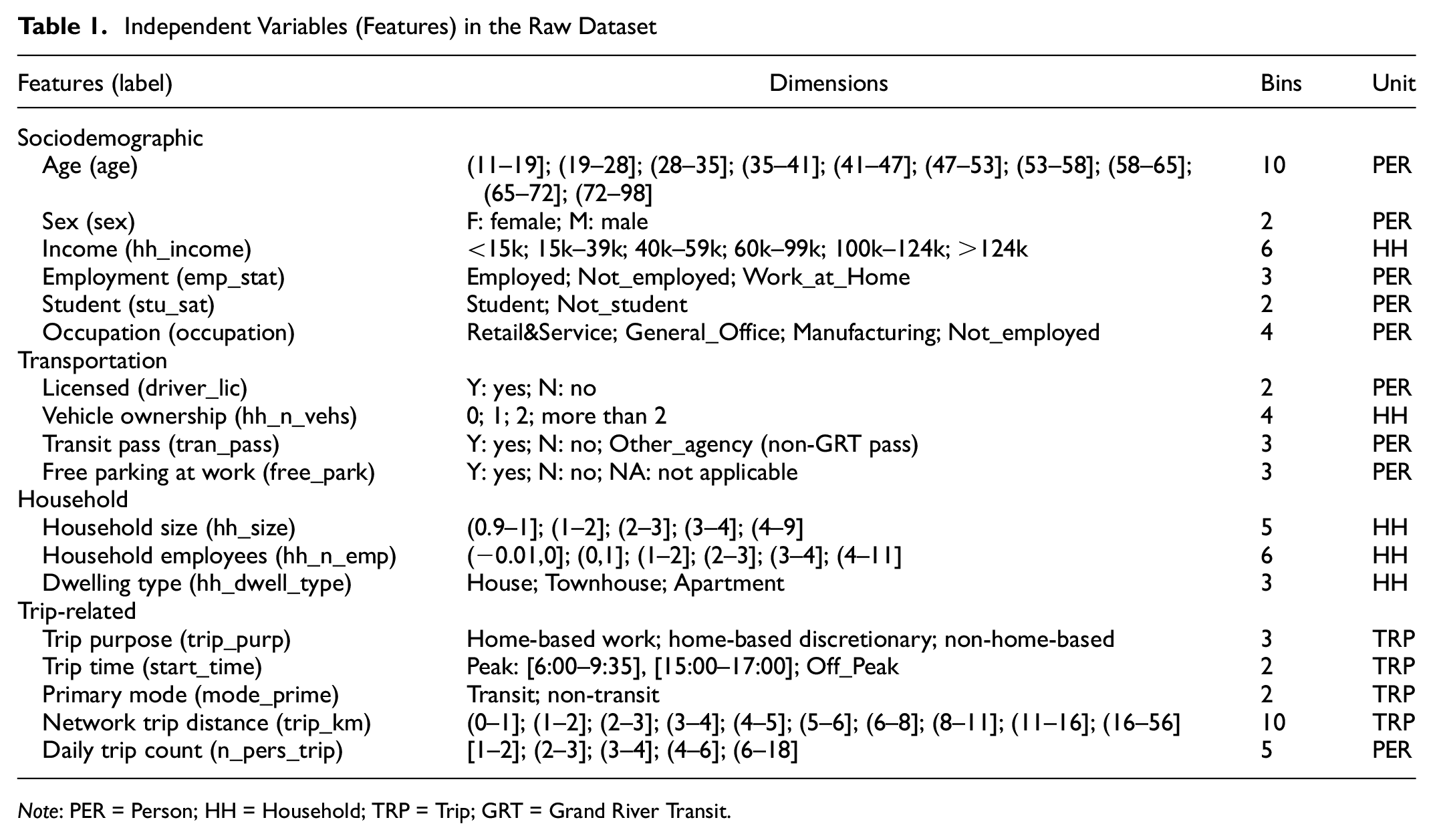
Note: PER = Person; HH = Household; TRP = Trip; GRT = Grand River Transit.
Figure 1 illustrates the observed missingness of the raw dataset, which contains a total of 51,104 trips conducted by households within the Region of Waterloo. The total raw dataset consists of 11,502 trips with at least one missing feature. Of the 18 features outlined in Table 1, the following seven features have incomplete observations: trip_km, age, driver_lic, trans_pass, emp_stat, occupation, and free_park. Of the missing features, hh_income and free_park have the highest proportions of incomplete observations totaling 16.1% and 7.7%, respectively.
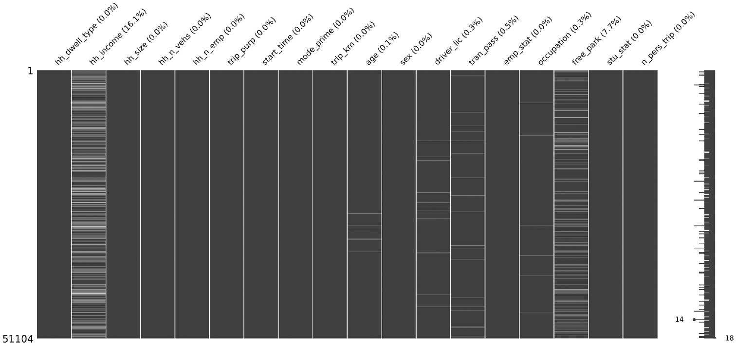
Observed missing data and missing proportions by feature (percentage of missing data).
Data Amputation for Simulation
A data amputation procedure is used to generate missing values in the processed dataset so that the performance of techniques can be evaluated. The data amputation aims to accurately reproduce the missing combinations, as summarized in Table 2, with the respective proportions to mimic the original dataset. This procedure allows the data imputation techniques to be tested on a representative dataset.
Missing Combinations of Raw Data (by Frequency)
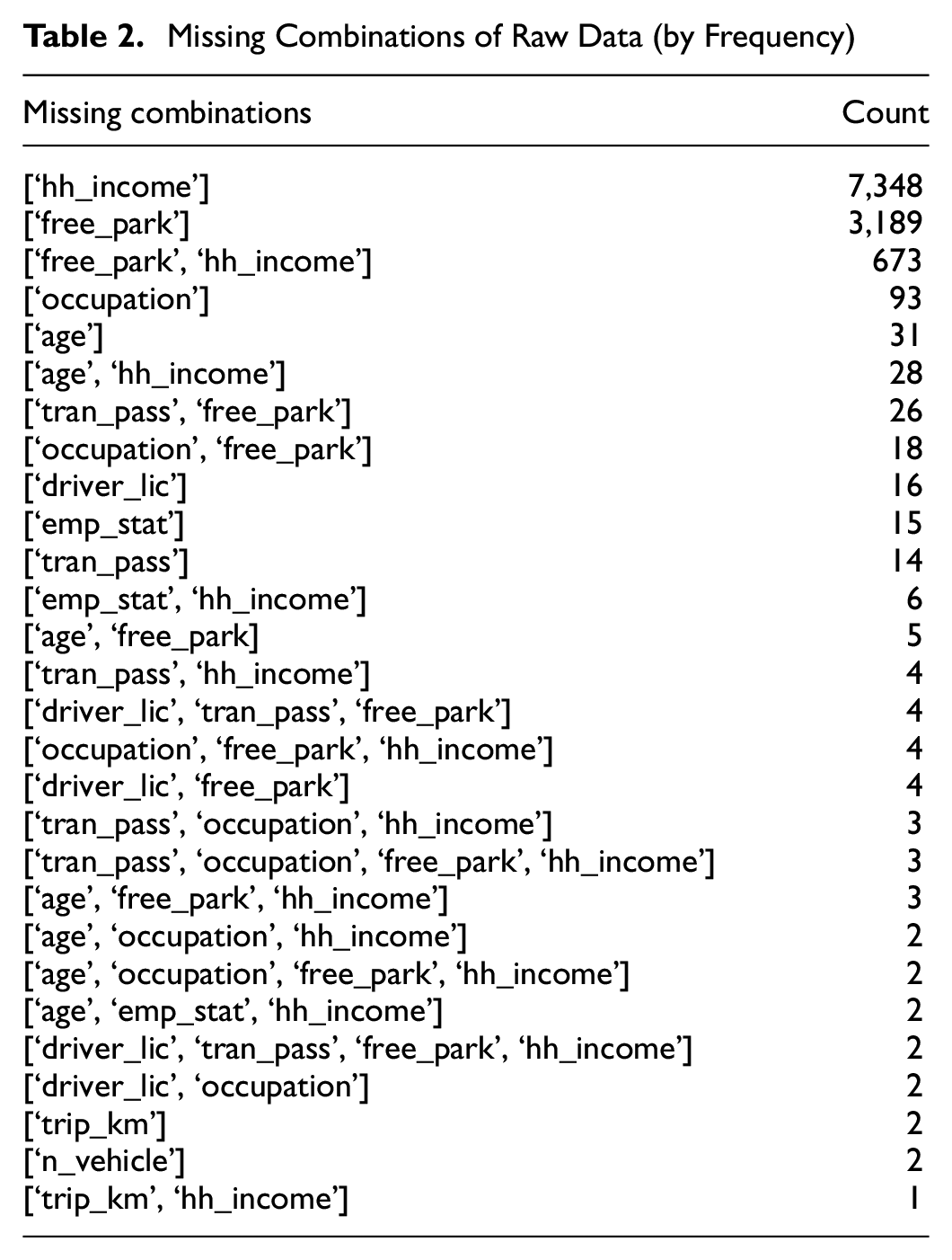
For this study, all records with missing items in the original survey dataset were deleted. The resulting dataset with fully known observations consists of 42,549 trips amongst 9,790 households. The amputation procedure starts at the household dataset and let this dataset with no missing values be called
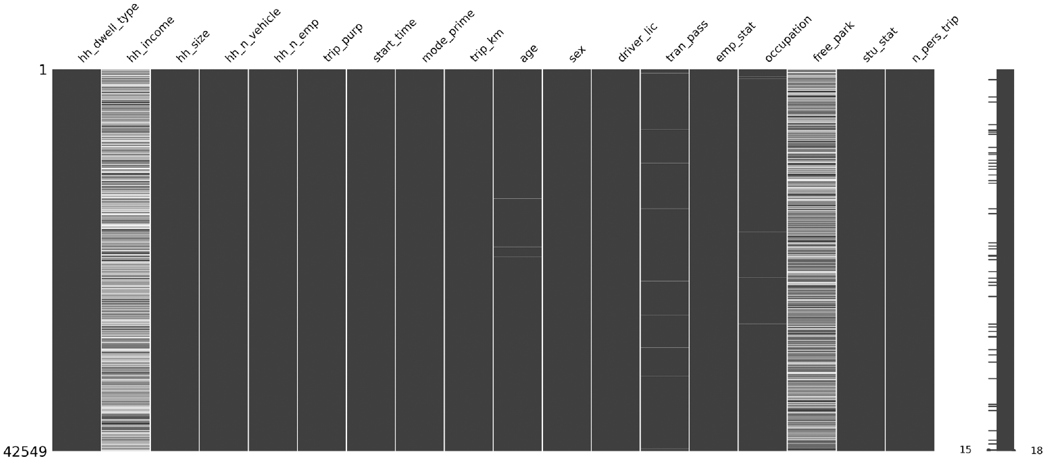
Simulated missing data for 50% missingness.
Data Imputation Techniques
Before testing the imputation techniques, all features were dummy encoded for preparation. The techniques utilized in imputing household travel survey data can be broadly classified into three categories: simple models, discriminative models, and generative models.
Multiple imputation—another popular imputation technique—is considered, but ultimately excluded from this study. Multiple imputation is sequential single imputation where several imputed versions of the incomplete data sets are first created by considering multiple candidates for each missing data point. The imputed sets of incomplete data are then evaluated using standard statistical procedures resulting in multiple different outcomes of the statistical analyses. Finally, these results are combined into an overall statistical analysis in which the uncertainty about the missing data is integrated in the standard errors and significance tests. A limiting factor of multiple imputation is the requirement of repeated imputation of the dataset, ultimately leading to a computationally expensive technique. Furthermore, it traditionally assumes a continuous metric for missing data and imputes continuous data, therefore converting categorical values into continuous ones. This assumption can cause problems with binary variables (e.g., free_park) by imputing a value of 0.8, thus creating impractical results. This problem would increase as the amount of missingness in the dataset increases. The fundamental concern of multiple imputation is that it fails to understand the meaning of the measure it is imputing where, even if no bias is present, it degrades the meaning of the considered variables ( 51 ).
Simple Imputation
The simple imputation methods used in this research are mode imputation and hot-deck imputation. Mode and hot-decking are simple imputation methods in which the missing values are filled by standard measure or constant. These methods do not require any training, since they instantly fill in the missing values based on simplistic calculations. Therefore, the dataset is not required to be dummy encoded for these methods. Both the methods are implemented using the scikit-learn library in Python 3.
Mode
Mode imputation replaces the missing values with the most frequent value in the column ( 52 ). It is the mean equivalent for the categorical variables. This method is a relatively common alternative to listwise deleting the missing data in the dataset. In this work, this approach is considered as the baseline method.
Hot-Deck Imputation
Hot-deck imputation is another simple imputation technique for filling missing data. It is especially useful for imputing missing data in large datasets ( 53 ). In this method, a missing item or value from a record (recipient) is replaced by a value from another similar case (donor) that has complete data.
For this study, the nearest neighbor (NN) hot-deck (k-NN) imputation is used, where a record with a missing value (recipient) is assigned the value of the NN case (donor) based on a distance metric. This imputation was conducted using the KNNImpute module from the scikit-learn library. This module carries out matrix completion of the data frame by choosing the mean values of the k closest samples for features where both samples are present. The distance metric used for this study was nan-Euclidean distance and only one neighbor was chosen for imputation.
Consider that a household survey case is represented by an n-dimensional input vector,
The nan-Euclidean distance between

where
This distance can either be 0 or 1 as all the features are categorical and dummy encoded. The weight term,
Discriminative Models
Discriminative models are models used for classification and regression. They study the probability of a class label,
For a simulated incomplete dataset,
For each feature in each combination of missing features in
After the models are trained, for each feature in each missing combination in
Overall accuracy of a feature is obtained by averaging the accuracy of all the different models used for that feature.
The above steps are conducted for all of the synthetic datasets.
This methodology was implemented with the scikit-learn library in Python 3.
Logistic Regression
This model is a generalization of the logistic regression model, which is used to model the relationship between a binary dependent variable and a set of

where
The left-hand side of the equation is also known as the binary logit model.
The simple logistic regression model can be generalized for multi-class dependent variables (multinomial logistic regression). For this case, with
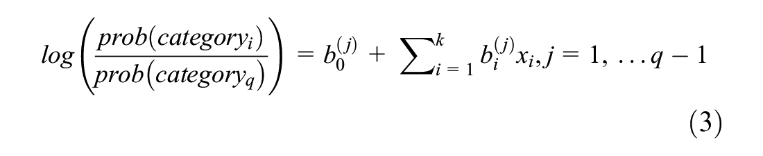
This model can be used for imputation by considering the dependent categorical variable with the missing value and all other features as the predictors.
Support Vector Machines (SVM)
SVM is another discriminative model used for imputation. This method takes a set of input data and predicts to which of one of the two possible classes each given input belongs. It does so by making a hyperplane that separates the data into two categories. The best separation is achieved by the hyperplane that has the largest distance to the nearest training data of any class (known as the margin), since the larger the margin, the lower the generalization error of the classifier ( 55 ). At times, the hyperplane will allow misclassifications, to prevent overfitting of the training data. In this case, the nearest training point to the hyperplane will be called a soft margin.
For a given dataset

where
In each case,
The optimization problem of SVM is as follows:
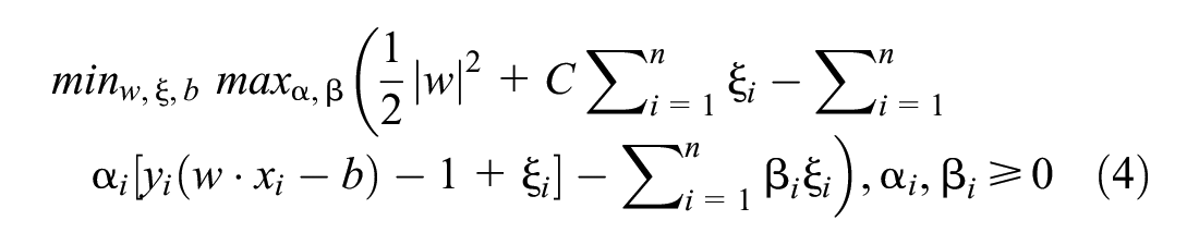
where
–
Other terms in the optimization problem are less critical hyperparameters and are left as default values ( 55 ).
For multiclass classification of
Multi-Layered Perceptron (MLP)
MLP is a neural network that consists of multiple layers of nodes interconnected in a feed-forward fashion. Each node or neuron is connected to the nodes of the next layer. These connections are called weights. The common MLP structure is made up of three layers: input layer, hidden layer, and output layer. The input layer connects the input data to the
For an input vector

where
The function

where
Since this study solely focuses on categorical variables, a logistic sigmoid was used as the

This study utilizes a two-layered MLP network (two hidden layers) as it is sufficient to model any complex relationships between the inputs and outputs ( 57 , 58 ). The network weights are found through model training on the Adam optimization method to minimize the cost function. Each hidden layer consists of 30 neurons based on a parameter sweep of hidden layer size (from 1 to 50). MLP networks can be used as an imputation technique by training the model to learn the missing features (used as outputs), using the remaining complete features as inputs ( 59 , 60 ).
Generative Model
Generative models capture the joint probability of
For a simulated incomplete dataset,
Create a corrupt set,
The
The percentage of missing data generated in set
The methodology is implemented where dataset X is not dummy encoded.
Autoencoders
Autoencoders are a type of neural network, having the same fundamental theory, that learn a distributed representation of their input ( 62 ). They transform the data into a smaller hidden layer, called the bottleneck layer, and reconstruct the entire dataset using the inputs from the bottleneck layer. By using a hidden layer (bottleneck) smaller than the input layer, the autoencoder learns the most important features present in the data.
For this study, an autoencoder with a categorical hinge cost is created between the reconstructed layer (output) and the input data, as it had the best performance. The weights and biases of the autoencoder are trained only on the complete dataset,
Measures of Effectiveness
Since the amputated dataset can provide a ground truth scenario, an objective metric is utilized for data imputation technique comparison. This study utilizes accuracy, shown in the formula below:

where
Results
Figures 3 and 4 summarize the accuracies of the six data imputation models across a percentage of missing data varying from 5% to 50% for high dimension and low dimension features, respectively. The baseline method of mode imputation is highlighted in Figures 3 and 4 with a dashed line type. The predictive accuracies of features with high dimensionalities, shown in Figure 3, reveal that autoencoders obtain the best overall averages accuracy of 84.1% (ranging from 33% to 100%). Apart from emp_stat, autoencoders perform significantly higher than the other five models. The SVM model typically follows autoencoders in relation to predictive accuracy averaging at 61.7% (ranging from 19% to 100%). The MLP and regression models then follow with average accuracies of 53.8% and 50.5%, respectively (both ranging from 0% to 100%). Lastly, the baseline mode imputation and k-NN performs with average accuracies of 46.8% and 48.4%, respectively (both ranging from 0% to 100%).
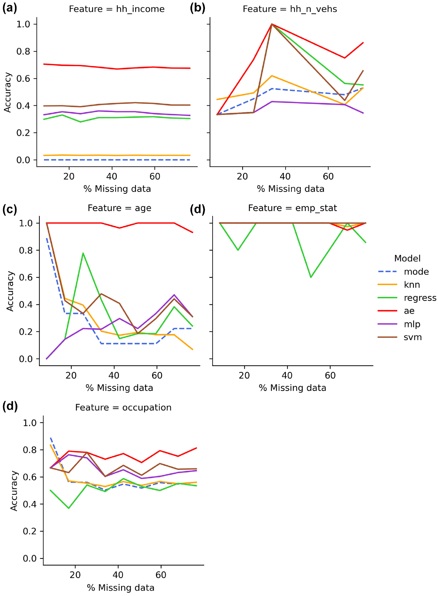
Comparative model performance for high dimension features: (a) income, (b) vehicle ownership, (c) age, (d) employment, and (e) occupation.
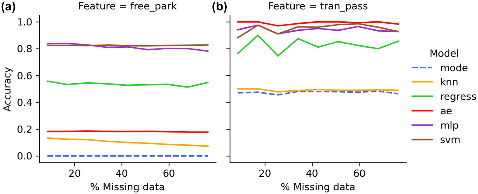
Comparative model performance for low dimension features: (a) free parking at work and (b) transit pass.
The predictive accuracies of features with low dimensionalities shown in Figure 4 reveal SVM and MLP models typically obtain the highest overall accuracies, averaging 88.7% (ranging from 82% to 99%) and 87.7% (ranging from 78% to 98%), respectively. Unlike high dimension features, the regression model performs with higher predictive accuracy and typically follows the SVM and MLP models averaging 68.1% accuracy (ranging from 51% to 90%). Unlike features with high dimensionality, the accuracy of autoencoders is inconsistent in performance and has a lower average accuracy of 58.7% (ranging from 18% to 100%). The k-NN performs poorly amongst the low dimension features with an accuracy averaging 29.7% (ranging from 5% to 50%). The baseline mode imputation performs at an average accuracy of 23.7% (ranging from 0% to 48%). Amongst the models that have average accuracies of 50% or higher, the autoencoder is the only model that has a higher predictive accuracies with higher dimension features than with lower dimension features.
For both high and low dimension figures, k-NN and mode imputation performed with very low accuracies overall with predictions of <5% accuracy for many features. It is also shown that the estimation accuracies of most features in all techniques do not show much impact with an increase in the percentage of missing data.
Discussion
Amongst the six methods assessed, autoencoders performed the best across varied missing data in datasets designed to be not at random. Furthermore, the performance, on average, for any of the models does not significantly change by the missingness of the dataset in the tested range (5%–50%), corresponding to previous findings from research on imputation in microarrays ( 64 ). Because of a low proportion of missingness in many features (e.g., emp_stat, hh_n_vehs), the training dataset for many machine learning models is limited. From the small training dataset, ranging the percentage of missing data may not cover critical amounts of data to warrant a change in predictive accuracies.
The results from autoencoders show limitations with low dimension features. A possible explanation might be not having optimal hidden layers and/or optimal neuron combinations, which could affect the model’s ability to optimally learn the latent space of the dataset. Better hypertuning of the hidden layer and neuron parameter may help with the model performance on features with binary classes. Additionally, the potential for autoencoders could be improved with further training, such as more epochs and less bottlenecking. Methods like MLP and SVM would be better suited to deal with features with low dimensions as seen through their performances. The remaining methods (mode, hot-deck, and logistic regression) are not recommended for imputation because of their poor performances on average.
Earlier research imputed one high dimension feature, number of cars, and one low dimension feature, drivers license, by utilizing SVM with inputs such as household composition, income, age, and so forth ( 13 ). Consistent with the findings of this study, their results reveal that the SVM performs better with lower dimension features (89% accuracy) than high dimension feature (69% accuracy) ( 13 ). When compared with the results of this study, the comparable feature of number of cars would be hh_n_vehs (33%–100% accuracy). Additionally, one previous study imputed an income feature through hot-deck and regression methods, finding better results with hot-deck than regression, which is also consistent with the findings of this study ( 6 ).
Although mode imputation is the simplest and easiest form of imputing data, it lowers the variability of the data and undermines the standard deviations and variances ( 65 , 66 ). While regression models utilize data from other variables used to predict the missing, it overestimates the correlations between predicted variables and its features while also underestimating variances and co-variances ( 65 ). Additionally, the hot-deck approach, commonly used in surveys, can bias the imputed results ( 53 , 67 ). The shortcomings of the aforementioned approaches present an opportunity for machine learning models where results are not biased. Consistent with the results of this research, machine learning methods outperform traditional statistical methods in imputing missing data, resulting in better overall accuracy because of their complex and flexible structure that allows for better pattern prediction and correlation detection ( 11 ).
This research is a promising step in using machine/deep learning techniques (both generative and discriminative) for missing data imputation for household surveys. All machine learning techniques are computationally expensive, some more so than others. Autoencoders are the fastest of the machine learning techniques to compute while the discriminative models take longer (SVM being the longest) because of the imputation scheme used for them. As the dataset size becomes larger, autoencoder time for training increases linearly; the same is true for the other neural network model, MLP. Models like SVM require computing a distance matrix, which increases exponentially in time.
Conclusion
In this study, the performances of six different imputation techniques are compared for household surveys. The six different imputation techniques include two simple imputation techniques (mode and hot-deck), three discriminative models (logistic regression, MLP, SVM) and one generative model (autoencoder). The assessment and comparison of these techniques resulted in several key findings. First, simple imputation techniques used previously in transportation, such as mode and hot-decking, performed considerably worse than the newer methods compared in this study (e.g., autoencoders, MLP, and SVM). Second, the dimensionality of the item had an impact on the most accurate imputation technique—for example, autoencoders performed very well with high dimensionality items, but less so with low dimensionality items. A related third finding is that the hypertuning of machine/deep learning techniques may require tailoring for specific items or for groups of items with similar dimensionality—of course, this can be done in practice the same way the techniques were assessed in this research (i.e., create a synthetic dataset with amputations). Fourth, imputation is generally more accurate with low dimension items compared with high dimension items. And fifth, the amount of missing data did not have a large influence on the accuracy of the imputation techniques in the ranges tested.
This research should be considered a first exploratory analysis of these methods. Future investigation is needed to confirm whether the performances shown by the machine learning models in this paper are a result of the structure of this specific household travel survey data or are suitable for generalization. Additionally, this study conducted imputation on the trip file, even for household characteristics, and some data imputation techniques such as hot-deck and regression imputation may perform better when applied at the household- and person- level files. Furthermore, because of spatial aggregation biases, spatial location is excluded from the original dataset. Further investigation with detailed spatial analysis to support data is noted as an opportunity for future research. The size of 42,549 cases is relatively large and methods may differ in performance with larger or smaller datasets. Similarly, investigation needs to be done on how the performance of the models might change if the continuous features were not binned and converted into categorical variables (where applicable). Lastly, detailed studies focused on hyperparameter tuning specifically for household travel survey data are warranted to determine if the tuning techniques used in other fields and adopted in this research are optimal for these data.
Footnotes
Author Contributions
The authors confirm contribution to the paper as follows: study conception and design: A. Budhwani, T. Lin, D. Feng, C. Bachmann; data collection: D. Feng; analysis and interpretation of results: A. Budhwani, T. Lin, C. Bachmann; draft manuscript preparation: A. Budhwani, T. Lin, D. Feng, C. Bachmann. All authors reviewed the results and approved the final version of the manuscript.
Declaration of Conflicting Interests
The author(s) declared no potential conflicts of interest with respect to the research, authorship, and/or publication of this article.
Funding
The author(s) received no financial support for the research, authorship, and/or publication of this article.