Sage Journals: Discover world-class research

Abstract

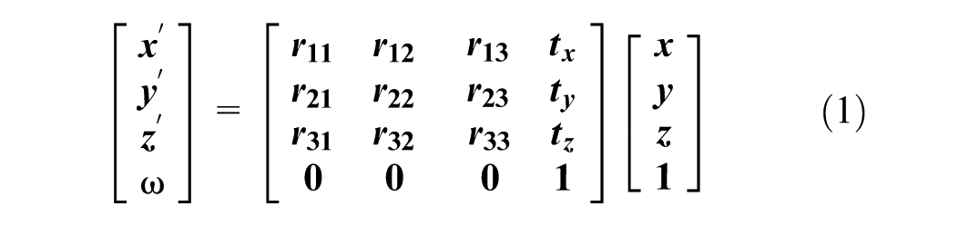
The FHWA classification scheme provides a standardized method for vehicle classification based on the number of axles and axle configuration, making it essential for effective traffic management, toll collection, and transportation planning. Although image-based classification methods have advanced significantly, they often struggle to accurately distinguish between certain FHWA vehicle classes using visual data alone. This challenge has led researchers to combine classes that are difficult to differentiate visually, thereby reducing the granularity and effectiveness of classification systems. In this research, we present a novel approach that enhances vehicle classification by leveraging the complementary strengths of both camera and LiDAR data. Because of the lack of existing fine-grained camera-LiDAR data sets for vehicle classification, we collected our own comprehensive dataset for the FHWA 13 classes. We employ a pretrained YOLOv8 model to detect and localize vehicles. Features from these localized images are extracted using a ResNet model. Simultaneously, the localized LiDAR point clouds are used to generate distance maps and calculate vehicle features such as length and height. The combined features and dimensions are input into a camera-LiDAR fusion multilayer perceptron classifier for final classification. To evaluate the performance of our proposed models, we employed metrics including recall, precision, and F1 score. Our comparative analysis demonstrates that the model fusing images and the distance maps yielded the highest performance, achieving a precision of 0.958, a recall of 0.932, and an F1 score of 0.938 across all classes.

Keywords

FHWA vehicle classification camera-LiDAR fusion vehicle detection sensor fusion supervised learning

Introduction

The FHWA introduced a standardized vehicle classification system in the mid-1980s to establish a uniform method for categorizing vehicles based on their physical and functional characteristics. This system organizes vehicles into 13 categories according to the number of axles, axle configurations, and spacing. Federal standardization of vehicle classifications ensures accurate traffic data collection and analysis, essential for various applications such as pavement design, highway maintenance scheduling, predicting commodity flows, highway capacity planning, and weight enforcement strategies ( 1 ). The detailed categorization enables precise differentiation between vehicle types. For instance, different truck classes are defined by the number of axles and their configurations, which influence pavement durability and infrastructure development. Figure 1 illustrates the FHWA vehicle classes, ranging from motorcycles (Class 1) to multitrailer trucks with seven or more axles (Class 13), facilitating detailed traffic analysis and management.

Figure 1.

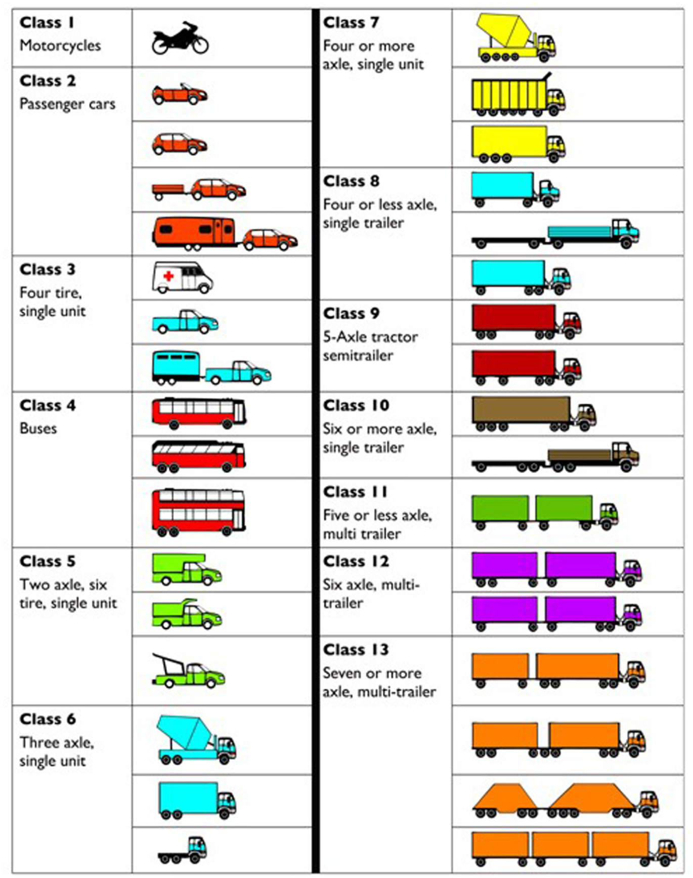
FHWA vehicle classification ( 2 ).

Traditional approaches to vehicle classification have primarily relied on inductive loop detectors, radar systems, and image-based methods. Inductive loop detectors, embedded in the road surface, measure changes in inductance caused by passing vehicles, providing reliable vehicle counts but limited classification capabilities ( 3 ). While dual-loop detectors can perform basic automatic classification, their performance is known to degrade on high-volume roads and their classification granularity is limited ( 4 ). Radar systems offer advantages in speed estimation but have limitations in dense traffic ( 5 , 6 ); however, modern frequency modulated continuous wave traffic radar sensors can detect both moving and stationary vehicles and are widely used for queuing and stop-bar detection ( 7 ).

On the other hand, image-based methods use cameras to capture visual data, which is processed to classify vehicles. While these methods have shown promise, they are sometimes challenged by varying lighting conditions and occlusions ( 8 ). Each of these traditional methods has its advantages and disadvantages. For instance, inductive loops are durable but require specialized expertise for installation, which can disrupt traffic flow during the process ( 5 ). In addition, radar systems can operate in various weather conditions but have limited classification granularity. To overcome the limitation of classification granularity, advanced sensor fusion approaches are being explored, combining multiple data sources to enhance vehicle classification accuracy.

Computer vision approaches have made significant strides in vehicle classification, leveraging deep learning models to achieve high accuracy. Models such as AlexNet ( 9 ) and VGGNet ( 10 ) influenced recent image classification by demonstrating the power of convolutional neural networks (CNNs) in extracting hierarchical features from images. These models were followed by more advanced architectures such as ResNet, which introduced residual connections to tackle the vanishing gradient problem. In the realm of vehicle detection and classification, models such as YOLO ( 11 ) and Faster R-CNN ( 12 ) have demonstrated impressive performance in detecting and classifying vehicles in real-time. These methods have excelled in scenarios with clear images and distinct vehicle features. However, they face challenges in distinguishing between vehicles with similar visual appearances, such as different models of sedans or trucks, especially when these vehicles have varying sizes ( 13 ). The lack of granularity in image-based classification can lead to misclassifications, influencing the effectiveness of traffic management systems. In addition, adverse weather conditions, poor lighting, and occlusions can further degrade the performance of these systems. To address these limitations, integrating a second modality, such as LiDAR, can provide additional spatial data, enhancing the robustness and accuracy of vehicle classification systems.

LiDAR technology has revolutionized several fields, including autonomous driving, robotics, and remote sensing, by providing precise 3D spatial data. LiDAR sensors emit laser pulses and measure the time it takes for the reflections to return, creating detailed point clouds that represent the environment ( 14 ). This technology’s strength lies in its ability to operate effectively in various lighting conditions and its capacity to capture minute details of objects’ shapes and sizes ( 15 ). LiDAR’s high spatial resolution and accuracy make it an ideal candidate for enhancing vehicle classification systems. By leveraging the detailed 3D data from LiDAR, we can accurately determine vehicle dimensions, such as length and height, which are challenging to extract from images alone. This capability is particularly beneficial for distinguishing between FHWA vehicle classes that are visually similar but differ in size. The integration of LiDAR data with camera data can significantly improve the granularity and accuracy of vehicle classification, addressing the limitations of image-only approaches.

The scope and objective of this study is to advance FHWA 13-class vehicle classification by addressing critical gaps in existing research, including the reliance on less granular data sets and the aggregation of vehicle classes. This research adds to the body of literature by introducing a custom LiDAR-camera data set that encompasses the FHWA axle-based vehicle classification scheme without aggregation and proposes a novel feature-level fusion framework that integrates camera and LiDAR data. By incorporating methodologies such as the use of distance maps and vehicle dimensions, this study presents a comprehensive and straightforward approach to dual-sensor vehicle classification, enhancing classification granularity and accuracy.

To achieve these objectives, this study develops three different approaches for our fusion methodology. Within this framework, we employ a pretrained YOLOv8 model for vehicle detection in images and use a ResNet model for feature extraction. In the first approach, the localized LiDAR point clouds are used to generate a distance map. This distance map is processed through a multilayer perceptron (MLP) to extract features, which are then concatenated with the image features obtained from the ResNet model. The combined features are input into an MLP classifier to predict the vehicle class. In the second and third approaches, the vehicle dimensions are calculated from the point cloud data. Each point in the point cloud is defined by its (x, y, z) coordinates, representing its position in 3D space. The vehicle length is determined by identifying the maximum and minimum points along the x-axis, which corresponds to the vehicle’s longitudinal axis. For the third approach, the height is also calculated using the maximum and minimum points along the z-axis, which corresponds to the vehicle’s vertical axis. These dimensions (length in the second approach, and both length and height in the third approach) are converted into feature vectors using an MLP. The resulting vectors are then concatenated with the image features extracted by the ResNet model and processed through the MLP classifier for final classification. The results are evaluated based on recall, precision, and F1 score, selected for their ability to provide a comprehensive assessment of classification performance. This research contributes significantly to three key aspects:

Comprehensive data collection: We collected extensive data using a Logitech C920 webcam and an Ouster OS2 LiDAR sensor mounted on a vehicle. This data set provides detailed information for FHWA classes, addressing the lack of fine-grained classification data sets for LiDAR and camera data.

Novel camera-LiDAR fusion methodology: We present an innovative approach that integrates camera and LiDAR data to improve vehicle classification accuracy. This fusion methodology combines vehicle dimensions from LiDAR with visual features from cameras within a robust framework.

Comparative analysis and evaluation: We conducted a comparative analysis of the three proposed models utilizing distance maps, vehicle length, and combined vehicle dimensions (length and height) from LiDAR data. Our evaluation metrics, including recall, precision, and F1 score, provide a comprehensive assessment of classification performance.

The rest of this paper is organized as follows. In the next section, we review existing literature on vehicle classification methods, highlighting their strengths and limitations. The following section describes our proposed fusion methodology in detail, including data collection, feature extraction, and classification techniques. The penultimate section explains the experimental setup, presents the results, and discusses the findings in the context of previous research. The final section concludes the study, summarizing the key contributions and suggesting directions for future research.

Literature Review

This literature review is structured into three subsections, starting with an examination of vision-based approaches, followed by an exploration of LiDAR-based methods, and concluding with a discussion of fusion-based approaches. Each method offers distinct advantages, with vision-based approaches being cost-effective, LiDAR providing comprehensive spatial information, and fusion integrating the strengths of both modalities.

Vision-Based Approach for Vehicle Classification

Vision-based methods utilize advancements in computer vision to detect and classify vehicles using 2D images. A prevalent limitation in many of these studies is the aggregation of FHWA classes into broader categories, which simplifies classification but compromises granularity and the ability to distinguish between similar vehicle types. Gothankar et al. ( 16 ) employed the MIO-TCD data set for vehicle detection using Tiny YOLOv3. To develop their wheel detection network, they sampled 2,500 images from 20 videos to classify vehicles into five axle-based classes (1-axle to 5-axle). Axles were detected using a CNN and the Circular Hough Transform, integrating multiobject detection with wheel detection to achieve an average accuracy of 89.4%. However, their classification system does not align with the FHWA’s 13-class scheme, particularly in distinguishing between different types of trucks. Similarly, Sasongko et al. ( 17 ) classifies vehicles into five groups (Nontruck, 2-Axle Truck, 3-Axle Truck, 4-Axle Truck, and 5-Axle Truck) using a fine-tuned CNN for image segmentation and pretrained ResNet model for classification. Their data set of 2,300 images, collected from toll roads and parking areas, achieved a high accuracy of 99%. However, their focus remained on simplified truck classes without addressing FHWA-specific distinctions, such as differentiating multitrailer trucks from single-unit trucks. Data set limitations are a recurring issue in vision-based approaches. Liu et al. ( 18 ) applied transfer learning to classify vehicles into four aggregated FHWA groups, namely Class 1, Classes 2–5, Classes 6–9, and Classes 10–12. Their method incorporated weak camera calibration and image-to-world homography for vehicle tracking and counting. However, their test data set contained only one vehicle in Class 10–12, revealing a significant class imbalance. Faster R-CNN performed better than YOLOv2 because of more precise bounding box detections, but the lack of representation for larger classes highlighted challenges in generalizability. Hussain et al. ( 19 ) explored vehicle-type classification with digital cameras, evaluating classifiers on downscaled, grayscale data sets. Using the BIT-Vehicle and LabelMe data sets, which include six categories (Sedan, Microbus, SUV, Bus, Minivan, and Truck), their ResNet model demonstrated superior performance, achieving an F1 score of 0.995. Efforts to improve classification under challenging conditions often remain constrained by non-FHWA data sets. Pemila et al. ( 20 ) classified vehicles into ten categories, including two-wheelers, three-wheelers, autos, buses, cars, and trucks, using wavelet transforms for feature extraction and XGBoost for classification. Their data set of 75,436 images achieved 98.81% accuracy but lacked adherence to the FHWA classification system. He et al. ( 13 ) focused on FHWA truck categories by detecting and counting axles, identifying trailers, and analyzing size and aspect ratios using deep learning. Their data set grouped trucks into nine FHWA-defined classes but also conducted a secondary 3-class experiment, combining Class 5–7, Class 8–10, and Class 11–13 for improved accuracy. The 9-class experiment achieved 91.32% accuracy, while the aggregated 3-class experiment yielded a higher accuracy of 96.34%, illustrating the difficulty of distinguishing visually similar vehicle types in the full FHWA scheme.

LiDAR-Based Approach for Vehicle Classification

LiDAR-based systems provide precise spatial measurements and detailed 3D modeling, which is essential for vehicle classification. Lee et al. ( 21 ) adopted a LiDAR-based system utilizing side-fire sensors to differentiate between vehicle and nonvehicle returns, cluster vehicles, identify occlusions, and classify nonoccluded vehicles into six categories. The system achieved over 99.5% accuracy but faced challenges in distinguishing commuter cars from motorcycles and encountered challenges with occlusions as a result of the sensor’s low height. Wu et al. ( 22 ) utilizes roadside LiDAR sensors, extracting six features from vehicle trajectories to classify them into ten FHWA-defined types. A data set of 1,056 samples was analyzed using Naïve Bayes, K-nearest neighbor, Random Forest (RF), and support vector machines. Among several machine learning models, RF achieved the highest accuracy, with a 91.98% success rate when vehicles were within 30 feet of the sensor. LiDAR’s capability for truck classification is highlighted in studies by Asborno et al. ( 23 ) and Vatani et al. ( 24 ). Asborno et al. ( 23 ) classified five-axle tractor-trailers into body types using LiDAR sensor to capture sparse point clouds, reconstructing dense 3D point clouds of trucks through a two-stage framework, and training a classification model with ensemble PointNet algorithms, achieving an 81% true positive rate and 87% volume accuracy, which correlated well with commodity flows on interstate and local roads. Similarly, Vatani et al. ( 24 ) employed pretrained CNN models such as AlexNet, VggNet, and ResNet to classify trucks with different trailers using 3D point cloud data. Their experiments demonstrated high feature extraction accuracy even with a small training data set. However, both studies primarily focused on truck-specific classifications, neglecting nontruck vehicle classes in the FHWA’s 13-class system. Some studies extend LiDAR applications beyond trucks to include other road users. Asborno et al. ( 23 ) classified motor vehicles, nonmotor vehicles, pedestrians, and bicyclists using point cloud data from roadside LiDAR sensors. Six features were manually extracted and used with machine learning algorithms, including support vector machine (SVM), RF, back propagation neural network (BPNN), and probabilistic neural network (PNN), to classify users into ten groups. These included eight FHWA vehicle classes and two additional classes for pedestrians and bicyclists. The SVM model with a Gaussian kernel achieved the highest F1 score of 84%, improving to 87.15% with reduced feature dimensionality. Yao et al. ( 25 ) and Dewan et al. ( 26 ) explored movement-based vehicle classification using LiDAR data. Yao et al. ( 25 ) employed airborne LiDAR with adaptive 3D segmentation and binary classification via SVM to distinguish between moving and stationary vehicles. They achieved absolute accuracy for object extraction scores of 83.2% and 81.7% and relative accuracy for object extraction scores of 82.7% and 84.5% on two data sets. In contrast, Dewan et al. proposed a pointwise semantic classification framework that categorized vehicles into three groups: nonmovable, movable, and dynamic. Their approach integrated semantic and motion cues using a deep neural network and a Bayes filter, achieving an F1 score of 84.44% on a standard benchmark data set. While both methods demonstrated effective movement-based classifications, neither addressed the detailed granularity required for FHWA’s 13-class axle-based system.

LiDAR and Camera Fusion-Based Approach for Vehicle Classification

Fusion approaches, combining visual and point cloud data, typically enhance vehicle classification by leveraging geometry and depth information. Fusion approaches are categorized by when the integration occurs, with early fusion combining raw sensor data, medium fusion merging feature representations, and late fusion integrating decision outputs from separate models. Using an early fusion approach, Niessner et al. ( 27 ) utilized red, green, and blue (RGB) and LiDAR data from an urban area data set provided by the IEEE Geoscience and Remote Sensing Society to detect vehicles, treating all vehicles as a single category without class distinctions. Three CNN training methods were evaluated, namely feature extraction with a pretrained CNN and SVM, fine-tuning a pretrained CNN, and training a CNN from scratch. An early fusion approach combining LiDAR intensity and elevation features at the input level achieved the highest F-Score of 0.927, outperforming models trained solely on RGB data, which yielded an F-Score of 0.722. Similarly, Gao et al. ( 28 ) trained their model on the RGB-LiDAR data set, which contains approximately 7,000 images categorized into pedestrians, cyclists, cars, and trucks. Each object is represented by RGB channels and an additional depth channel. This approach achieved an average accuracy of 96% by integrating pixel-level upsampled LiDAR depth information with RGB data and processed it through a CNN. At the decision level, Liu et al. ( 29 ) utilized sparse LiDAR point cloud data, which was denoised and ground-separated before applying a clustering algorithm to identify surrounding vehicles. The processed LiDAR data was fused with classification outputs from a neural network trained on image data. This method, which treated all vehicles as a general category without specific classifications, achieved an average accuracy of 85.5% for obstacle detection. The approach demonstrated the effectiveness of decision-level fusion in a cost-effective sensing setup, validated through real-field testing. Oh et al. ( 30 ) evaluated a decision-level fusion method on the KITTI benchmark data set, which includes categories for cars, pedestrians, and cyclists. The approach combined outputs from 3D LiDAR point clouds and image data processed by a five-layer CNN. Pretrained convolutional layers and region of interest (ROI) pooling were used to enhance data representation for both LiDAR and charge-coupled device (CCD) sensors. The method achieved a mean average precision of 77.72%, demonstrating the effectiveness of decision-level fusion for multiclass detection and classification. Using a feature-level fusion, Lee et al. ( 31 ) used a multistage method for 3D object detection and classification on a data set of 6,680 frames categorized into vehicles, pedestrians, and cyclists. The approach applied a LiDAR-based centerpoint-pillars detector with pillar feature encoding, a ResNet50-Tiny backbone, and a detection head. Camera calibration parameters projected 3D bounding boxes onto images, followed by camera-based image classification to refine results and eliminate false positives. The method achieved 91.48% accuracy and 78.1% balanced accuracy.

The scope of this study focuses on enhancing FHWA 13-class vehicle classification by addressing limitations in prior works that relied on less granular data sets or aggregated vehicle classes. Unlike previous studies, our work uses a custom, fine-grained data set collected with a Logitech C920 webcam and an Ouster OS2 LiDAR sensor, covering the 13 FHWA vehicle classes without any class aggregation. This data set enables precise evaluation of classification systems, particularly for visually similar classes that are often challenging to distinguish. This research introduces a novel, feature-level fusion methodology that integrates detailed vehicle dimensions, such as length and height, and distance maps generated from localized LiDAR point clouds with visual features extracted from cameras. These approaches provide a comprehensive yet straightforward framework for camera-LiDAR fusion, designed to address the challenges of vehicle classification accuracy and granularity. By leveraging these distinct fusion strategies, our study contributes a new method to the domain, providing an alternative to existing techniques that primarily focus on either aggregated classes or more complex fusion processes.

Data Set

Camera and LiDAR Data Collection

In this study, we utilized the Ouster OS2 360-degree LiDAR, which generates substantial data because of its wide scanning range. To manage the large volume of data and enhance processing efficiency, we filtered out irrelevant point cloud data. Specifically, we retained only the point clouds within the ROI area. By assessing the bird’s-eye view of the map, we determined that the furthest point of interest on the highway was approximately 62 m from the LiDAR. Consequently, we established a filtering range of 70 m to effectively exclude any points beyond this range, thus removing unnecessary background data such as trees.

In this study, an OUSTER OS2 64-channel LiDAR, which provides a detection range of 200 meters at 10% reflectivity and a maximum range of 400 m was utilized. The OS2 LiDAR features a 22.5° vertical field of view and a 360° horizontal field of view. It operates with 128 channels of resolution, capturing up to 2.62 million points per second at a maximum frame rate of 20 Hz, enabling detailed and comprehensive 3D data acquisition. In addition, a Logitech 1080p Webcam, which provides a camera resolution of 640×480, 90-degree field of view and operates at a frame rate of 30 Hz was installed on the LiDAR unit and positioned to face the Interstate 70, where the speed limit is 70 mph, from a parking lot. The LiDAR and camera devices were positioned at an optimal height of approximately 3 m and at a distance of 40 to 70 m away from Interstate 70 to ensure a broader field of view in the camera images, thereby reducing the likelihood of missed detections. Before data collection, the LiDAR and camera were oriented toward the roadway using a level measurement app and a compass app on an iPhone, and cross-checked with the roadway heading from Google Maps. This procedure ensured basic alignment between the LiDAR x-axis and the traffic flow direction.

As shown in Figure 2, this simple setup, using LiDAR as a stable base for the camera, enabled the concurrent collection of point cloud and image data on Interstate 70 with synchronized timestamps, making the process accessible and efficient for researchers without requiring specialized expertise. The entire system was operated using the Robot Operating System, which enabled synchronized data collection from both sensors. Given the 360-degree horizontal field of view of the OUSTER LiDAR, only the points within the ROI were cropped to fuse with the image data. The data was collected over three separate one-hour sessions, each limited by the Ouster LiDAR’s battery capacity.

Figure 2.

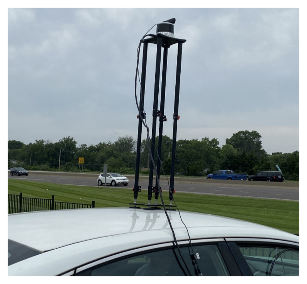
LiDAR and camera system setup for data collection.

Data Description

Following collection, video data were processed into individual frames, with consecutive frames showing the same vehicles removed to reduce unnecessary repetition. In addition, frames containing only Class 2 vehicles, which were already overrepresented, were selectively excluded to improve class balance. Figure 3 illustrates the distribution of image counts across the 13 FHWA vehicle classes in our data set. The data set reveals significant variability in the number of images per class. Notably, Class 2, representing passenger cars, dominates the data set with nearly 2,000 images. This is followed by Class 3, which includes two-axle, four-tire, single-unit vehicles, with over 1,000 images. Other classes, such as Class 5 and Class 9, also have substantial representation, with each containing several hundred images. However, many classes, including Class 1, Class 4, and Classes 6 through 12, exhibit much lower frequencies, with some classes having fewer than 100 images. It is important to note that there were no vehicles obtained for Class 7 and Class 13. Consequently, these classes were omitted from both training and testing phases. Figure 4 provides a sample of localized images for each of the 13 FHWA vehicle classes, illustrating the diversity of vehicle types included in the data set.

Figure 3.

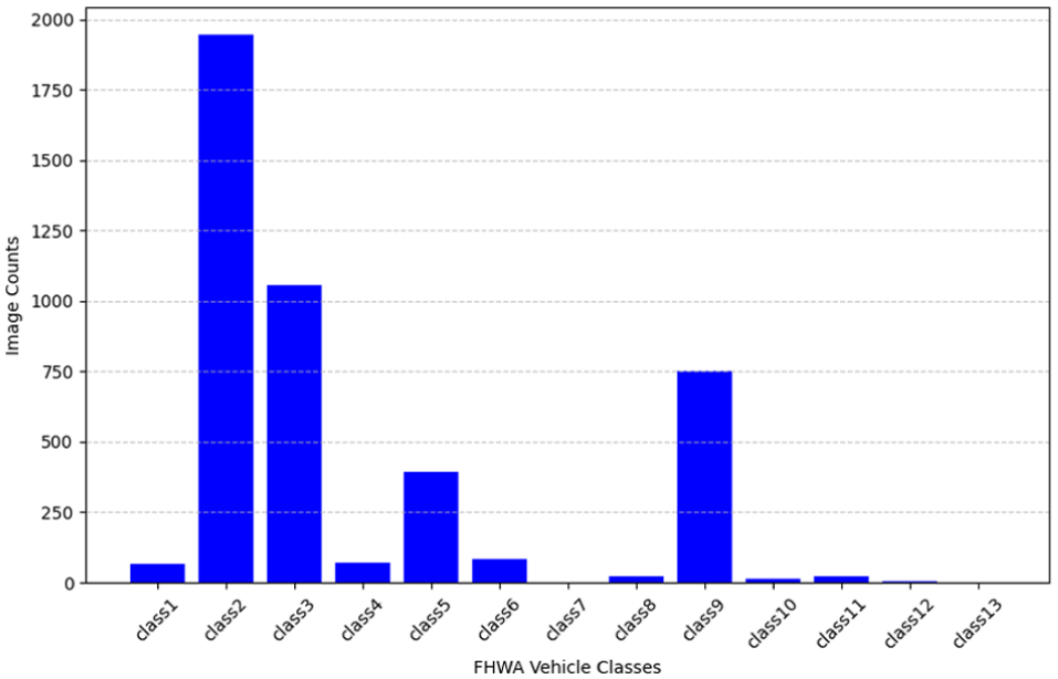
Distribution of LiDAR and image data among FHWA classes.

Figure 4.

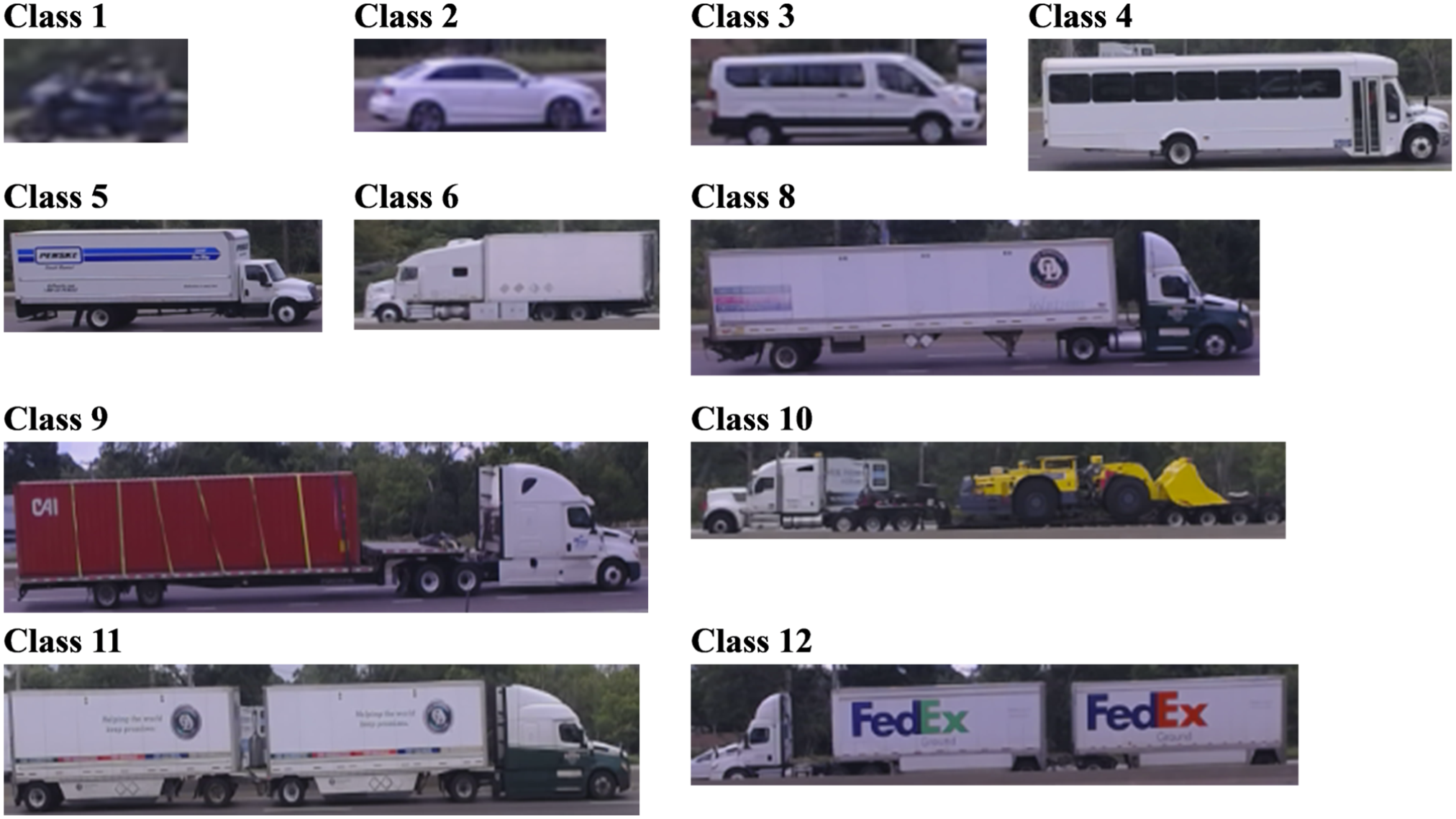
Sample of localized image in each of the 13 FHWA vehicle classes.

Because of data set imbalance from collecting data primarily on a single highway dominated by passenger cars, we recommend counteracting this by obtaining additional data from locations with higher truck traffic, such as industrial areas, ports, distribution centers, or weighing stations. To further enhance the data set’s diversity without extensive resource allocation, implementing oversampling strategies for underrepresented classes is advisable. While data augmentation techniques such as rotations and scaling are feasible for LiDAR data, caution is necessary in a camera-LiDAR fusion context, as these methods might disrupt the synchronization between modalities and compromise data integrity.

Camera and LiDAR Data Synchronization

The LiDAR point cloud, a collection of data points in a 3D coordinate system, captures attributes such as shape, position, color, distance, and intensity. To ensure accurate data fusion for vehicle classification, it is essential to synchronize the data from the camera and LiDAR sensors. Our setup involved a camera operating at 30 frames per second (fps) and a LiDAR sensor operating at 20 fps. This discrepancy in frame rates necessitated careful preprocessing to achieve synchronization.

The initial step in this process is temporal alignment, matching each camera frame with the corresponding LiDAR frame based on their timestamps. This temporal synchronization ensures consistent data fusion despite the frame rate mismatch. Following temporal alignment, spatial synchronization is performed by transforming the LiDAR points to align with the camera’s perspective. This involves applying calibration between 3D LiDAR points (x, y, and z coordinates) and 2D images. The calibration, composed of intrinsic calibration and extrinsic calibration, converts LiDAR points from the LiDAR coordinate system to the camera coordinate system, ensuring spatial alignment. Intrinsic parameters define the camera’s internal characteristics, such as focal length and optical center, while extrinsic parameters describe the transformation between the 3D points from the LiDAR sensor and the pixels from the camera sensor.

The Ouster OS2 360-degree LiDAR generates substantial data because of its wide scanning range. To manage the large volume of data and enhance processing efficiency, we filtered out irrelevant point cloud data. Specifically, we retained only the point clouds within the ROI area. By assessing the bird’s-eye view of the map, we determined that the furthest point of interest on the highway was approximately 62 m from the LiDAR. Consequently, we established a filtering range of 70 m to effectively exclude any points beyond this range, thus removing unnecessary background data such as trees.

Projecting 3D point cloud data onto the 2D image plane typically involves utilizing a $4 \times 4$ transformation matrix, which is composed of a $3 \times 3$ rotation matrix and a $3 \times 1$ translation vector. Equation 1 demonstrates this process, where $r_{11}$ to $r_{33}$ denote the components of the rotation matrix, while $t_{x}$ to $t_{z}$ represent the elements of the translation vector. The homogeneous coordinate $ω$ is included to facilitate the projection and normalization procedures. As illustrated in Equation 1, solving for the 12 unknown parameters of this transformation requires a minimum of six pairs of corresponding points between the 3D point cloud and the 2D image plane.

[\begin{matrix} x^{'} \\ y^{'} \\ \begin{matrix} z^{'} \\ ω \end{matrix} \end{matrix}] = [\begin{matrix} \begin{matrix} r_{11} r_{12} \\ r_{21} r_{22} \end{matrix} \begin{matrix} r_{13} t_{x} \\ r_{23} t_{y} \end{matrix} \\ \begin{matrix} r_{31} r_{32} \\ 0 0 \end{matrix} \begin{matrix} r_{33} t_{z} \\ 0 1 \end{matrix} \end{matrix}] [\begin{matrix} \begin{matrix} x \\ y \end{matrix} \\ \begin{matrix} z \\ 1 \end{matrix} \end{matrix}]

(1)

By applying the transformation matrix, we transform and rotate the LiDAR points based on the camera’s position and project them onto the 2D image plane. To validate our synchronization and calibration, Figure 5 displays the superimposition of LiDAR point clouds onto camera images. This visual representation demonstrates the effectiveness of our synchronization process, with the point clouds accurately overlaying the corresponding vehicles in the images.

Figure 5.

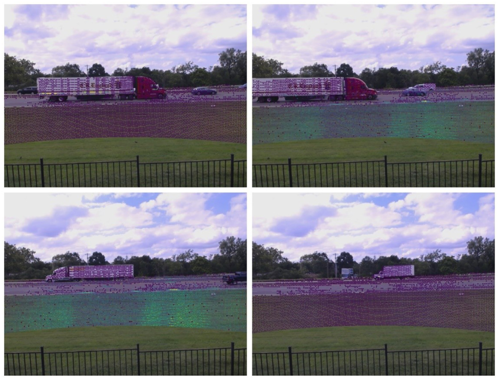
LiDAR point clouds superimposed on camera image to visualize dual-sensor data synchronization.

The LiDAR and camera were positioned about 40–70 m from Interstate 70. In the data processing stage, only vehicles in the near lanes were retained, as those farther away often suffered from significant occlusion. The usable data therefore mainly represent vehicles at an effective distance of roughly 40 m from the sensors. At this range, based on the intrinsic parameters of the 640×480 camera and its extrinsic calibration with the LiDAR, each pixel corresponds to about 7.8 cm in both horizontal and vertical directions. Under this geometry, the full image covers approximately 49.9 m across the roadway laterally and 37.5 m vertically, providing sufficient coverage for vehicle observations.

Methodology

In this research, we propose a novel framework that integrates camera and LiDAR data to enhance the accuracy of FHWA axle-based vehicle classification, employing three distinct fusion approaches. Initially, a pretrained YOLOv8 model detects vehicles in images, and a ResNet model extracts features from these localized images. As depicted in Figure 6, the first approach, localized LiDAR point clouds are used to generate a distance map, which is then processed through an MLP to extract features. In the second approach, vehicle length is calculated from the point cloud data by identifying the maximum and minimum points along the vehicle’s longitudinal axis (x-axis). As shown in Figure 7, the third approach extends the second by also calculating vehicle height using the vertical axis (z-axis) in the point cloud data. The extracted features (distance map, length, and height) are converted into feature vectors using an MLP. These vectors are concatenated with the image features from the ResNet model. The combined features are then input into a final MLP classifier to predict the FHWA vehicle class.

Figure 6.

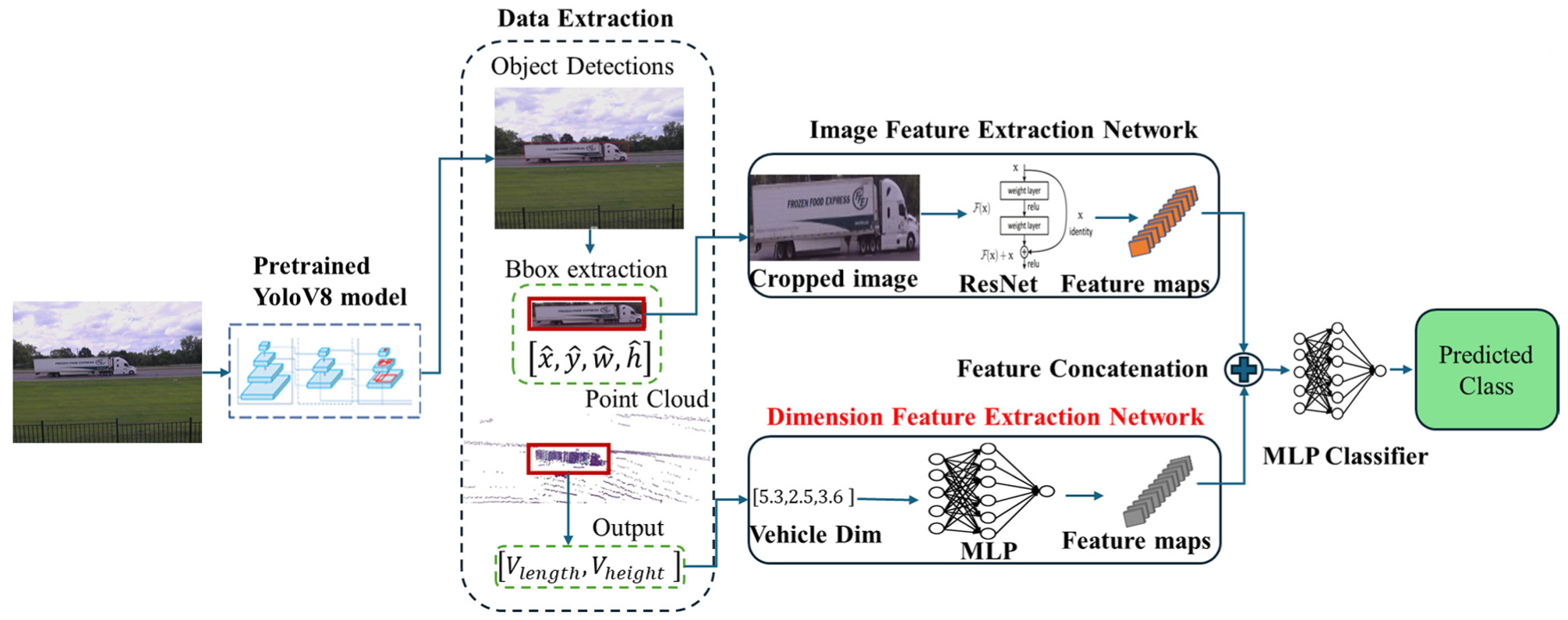
Proposed camera-LiDAR fusion framework using vehicle dimensions.

Figure 7.

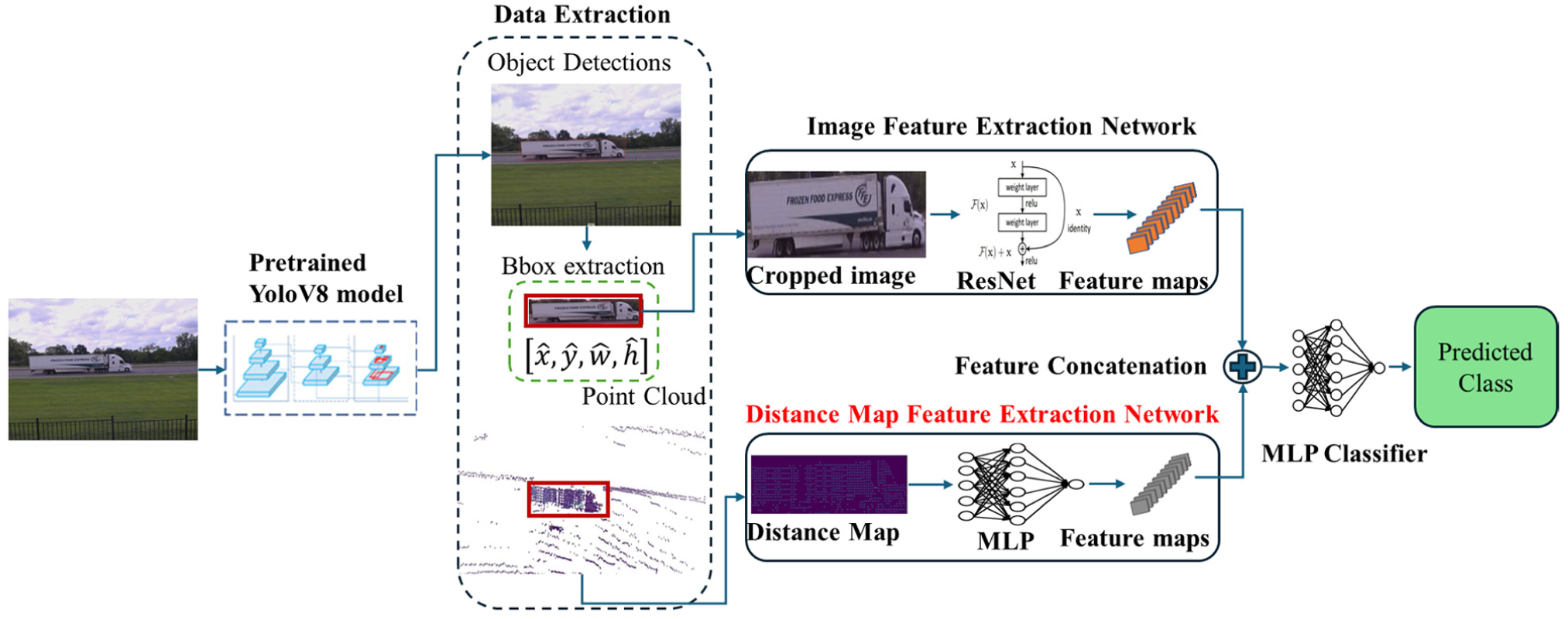
Proposed camera-LiDAR fusion framework using distance map.

Pretrained Yolov8

In our framework, a pretrained YOLOv8 ( 32 ) model is employed to generate bounding box coordinates that are subsequently used to localize vehicles in both the images and their corresponding LiDAR point clouds, thereby forming the foundation for subsequent feature extraction. YOLOv8 is a state-of-the-art single-stage object detection algorithm known for its balance of speed and accuracy.

The architecture of YOLOv8, as illustrated in Figure 8, consists of two main components: the Backbone and the Head. The Backbone captures multiscale visual representations through convolutional layers and C2f blocks that integrate convolutional and bottleneck modules to merge high-level features with contextual information, along with a spatial pyramid pooling – fast (SPPF) module that enhances spatial context through pyramid pooling, and a Head that processes these outputs to produce bounding box and class predictions. The Head of YOLOv8 processes the features from the Backbone through a combination of convolutional, C2f, and upsampling layers to generate box and class predictions. Key innovations in YOLOv8, such as anchor-free detection, mosaic augmentation, and self-adversarial training, contribute to its efficiency and effectiveness. It should be noted that our evaluation assesses classification performance only on vehicles successfully detected by YOLOv8, which represented the majority of vehicles in the data set.

Figure 8.

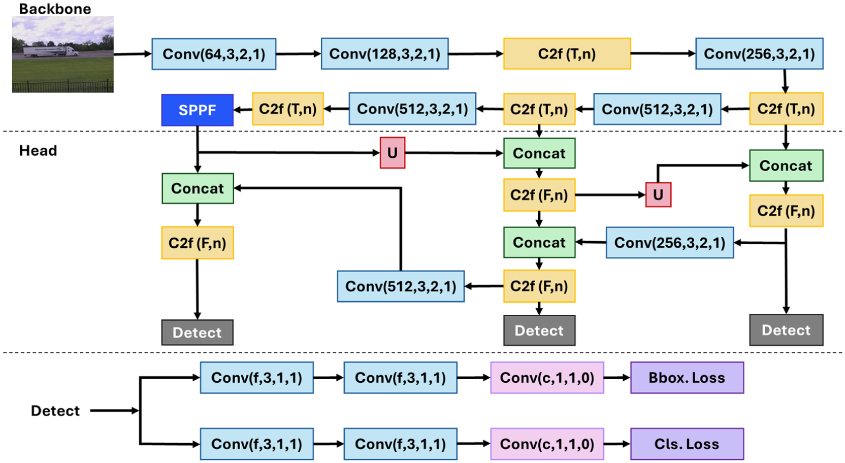
YOLOv8 model structure ( 33 ).

Image Feature Extraction

After vehicle localization with YOLOv8, the cropped images are passed through a ResNet model to extract feature maps. ResNet ( 34 ) is a robust deep learning architecture designed to overcome the vanishing gradient problem, which can impede the training of deep networks. It achieves this through residual learning, where shortcut connections bypass one or more layers, enabling the network to learn residual functions relative to the layer inputs. The core component of ResNet is the bottleneck block, comprising three convolutional layers: a 1×1 convolution for dimensionality reduction, a 3×3 convolution for feature processing, and a final 1×1 convolution to restore dimensionality. Each convolutional layer is followed by batch normalization and ReLU activation. The shortcut connections facilitate direct gradient flow through the network, allowing the construction of much deeper architectures, which leads to enhanced performance on various tasks. As depicted in Figure 9, the ResNet model starts with an initial convolutional layer and a max-pooling layer, followed by multiple stages of bottleneck blocks that increase in depth and complexity. This is followed by an adaptive average pooling layer and a fully connected layer that produces the final feature maps. These feature maps are then utilized in our camera-LiDAR fusion model for further processing and classification.

Figure 9.

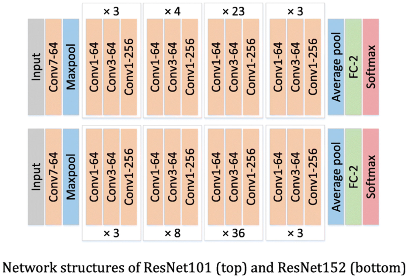
ResNet-152 architecture ( 35 ).

Distance Map Feature Extraction

The distance map is generated by computing the Euclidean distance from a reference point within each localized vehicle point cloud to all other points in that same point cloud. The reference point is selected as the top-left corner point of the vehicle’s bounding box in the cropped point cloud data. The distance is calculated using

d = \sqrt{{(x - x_{0})}^{2} + {(y - y_{0})}^{2} + {(z - z_{0})}^{2}}

(2)

where d = distanc; and $x_{0}$ , $y_{0}$ , and $z_{0}$ = coordinates of the reference point. The resulting distances are stored in a 2D grid to represent spatial distribution and depth. These maps are then input into an MLP for feature extraction, preserving 3D geometric details of the vehicle.

Vehicle Dimension Feature Extraction

The LiDAR point cloud data, localized within bounding boxes around detected vehicles, is used to extract vehicle dimensions, specifically length and height. The vehicle length is determined by identifying the maximum and minimum points along the longitudinal axis (x-axis), while the height is calculated using the maximum and minimum points along the vertical axis (z-axis). These dimensions provide critical geometric information about the vehicle. The extracted length and height features are converted into feature vectors using an MLP.

Final MLP Classifier

The final classification in our framework is performed by an MLP classifier that combines features from both image and LiDAR data. Image features extracted using a ResNet152 backbone with a dimensionality of 2048 are concatenated with LiDAR features processed through a convolutional network with a dimensionality of 64. The combined feature vector with a dimensionality of 2112 is passed through a series of fully connected layers that sequentially reduce the dimensions to 512, then to 256, and finally to the number of vehicle classes. Each layer incorporates ReLU activation and LayerNorm with dropout applied for regularization. The output of the classifier is a vector of class probabilities, indicating the likelihood of the input belonging to each vehicle class. This architecture effectively utilizes the combined features from both sensors for accurate vehicle classification.

Baseline Models for Comparison

Three baseline models were employed for comparison: RGB ResNet, red, green, blue, and depth (RGBD) ResNet, and PointFusion. The RGB ResNet model, based on the ResNet152 architecture, processes standard three-channel RGB images and serves as a baseline for image-only classification. The RGBD ResNet model extends this architecture to handle four-channel RGB-D inputs by modifying the initial convolution layer to process depth information alongside RGB data. This modification allows the model to incorporate geometric features in addition to visual information. Lastly, the PointFusion model integrates RGB images and 3D LiDAR point clouds, extracting features from images using a ResNet152 backbone and from point clouds using a PointNet architecture. These features are concatenated and passed through an MLP for classification, utilizing complementary visual and spatial data. These models were selected to provide a robust baseline for evaluating the performance of our proposed fusion framework.

Experiment and Results

Training and Validation

In this study, the performance of the fusion model was evaluated using different feature sets. Model training and testing were achieved using an Alienware m16 R1 system equipped with NVIDIA GeForce RTX 4080 GPU (12 GB VRAM) and CUDA 12.6 support. The data set was divided into training, validation, and test sets with a split ratio of 70% for training, 15% for validation, and 15% for testing. All localized images were resized to 224×224 pixels to ensure consistency in input dimensions. The loss function used for training was cross-entropy loss, which is suitable for multiclass classification tasks as it measures the performance of a classification model whose output is a probability value between 0 and 1. As shown in Equation 3, cross-entropy loss penalizes the deviation of the predicted probability from the true class label, thus effectively guiding the optimization process. The formula for cross-entropy loss is given by

L = - \frac{1}{N} \sum_{i = 1}^{N} \sum_{c = 1}^{C} y_{ic} \log (\hat{y_{ic}})

(3)

where $N$ = number of samples; $C$ = number of classes; $(y_{ic})$ = binary indicator (0 or 1) if class label $(c)$ is the correct classification for sample $(i)$ ; and $(\hat{y_{ic}})$ = predicted probability that sample $(i)$ belongs to class $(c)$ .

The hyperparameters for each model were independently tuned to optimize performance. Table 1 outlines the specific hyperparameters used for each model. Early stopping with a patience of 10 was employed during training. The proposed models were trained for 50 epochs, while the baseline models were trained for 100 epochs to achieve optimal performance.

Table 1.

Hyperparameter for Each Model

Model	Epochs	Batch size	Learning Rate	Optimizer
Fusion model using length	50	16	0.001	AdamW
Fusion model using size	50	16	0.001	AdamW
Fusion model using distance map	50	16	0.001	AdamW
RGB ResNet	52	24	0.00001	AdamW
RGBD ResNet	44	24	0.00001	Adam
PointFusion	33	10	0.00001	AdamW

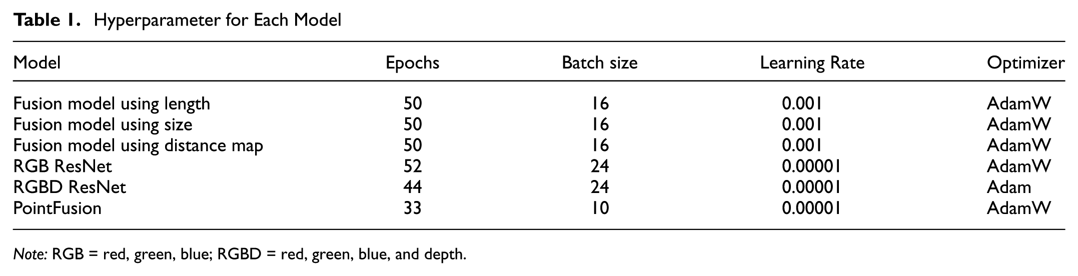
Note: RGB = red, green, blue; RGBD = red, green, blue, and depth.

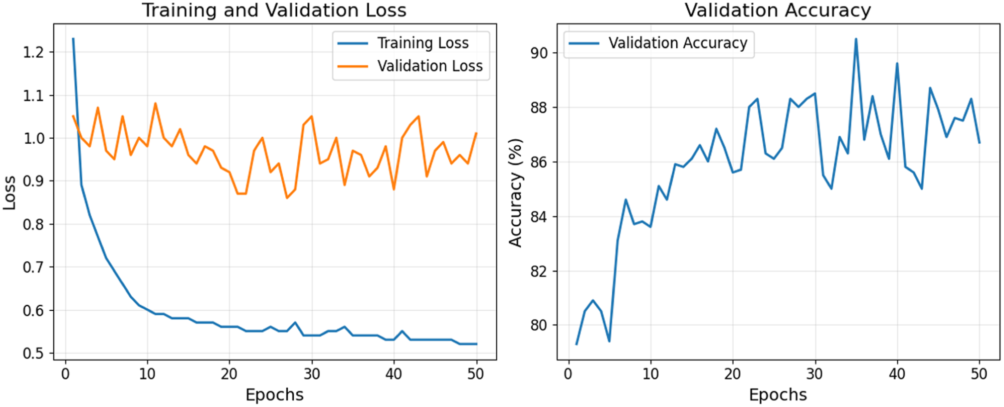
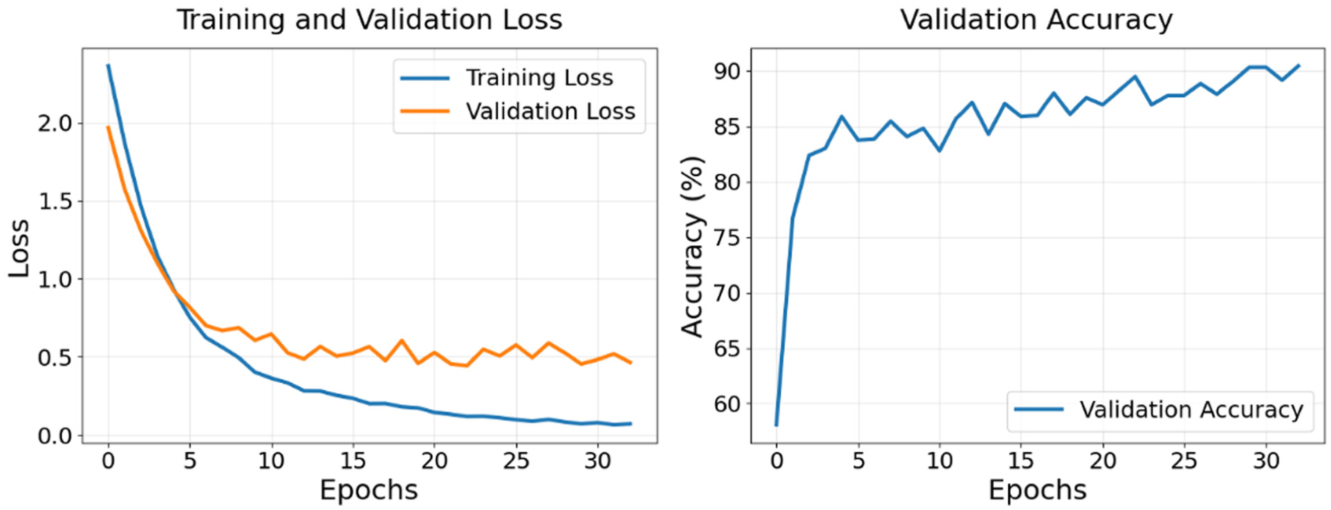
Figures 10 –15 illustrate the training and validation loss (left) and validation accuracy (right) for the models. Both the proposed models (Figures 10 –12) and the baseline models (Figures 13 –15) show consistently decreasing training loss, indicating effective optimization. The validation loss also decreases across all models, with some fluctuations, reflecting efforts to minimize error on unseen data. Validation accuracy improves during the early epochs and stabilizes over time for all models, demonstrating their ability to generalize effectively to validation data. It should be noted that the y-axis scales are not identical across figures, as the models converge within different ranges, and uniform scales would suppress meaningful fluctuations. The figures are therefore intended to illustrate each model’s convergence and the improvement of validation accuracy with increasing epochs, rather than to enable direct visual comparisons across models.

Figure 10.

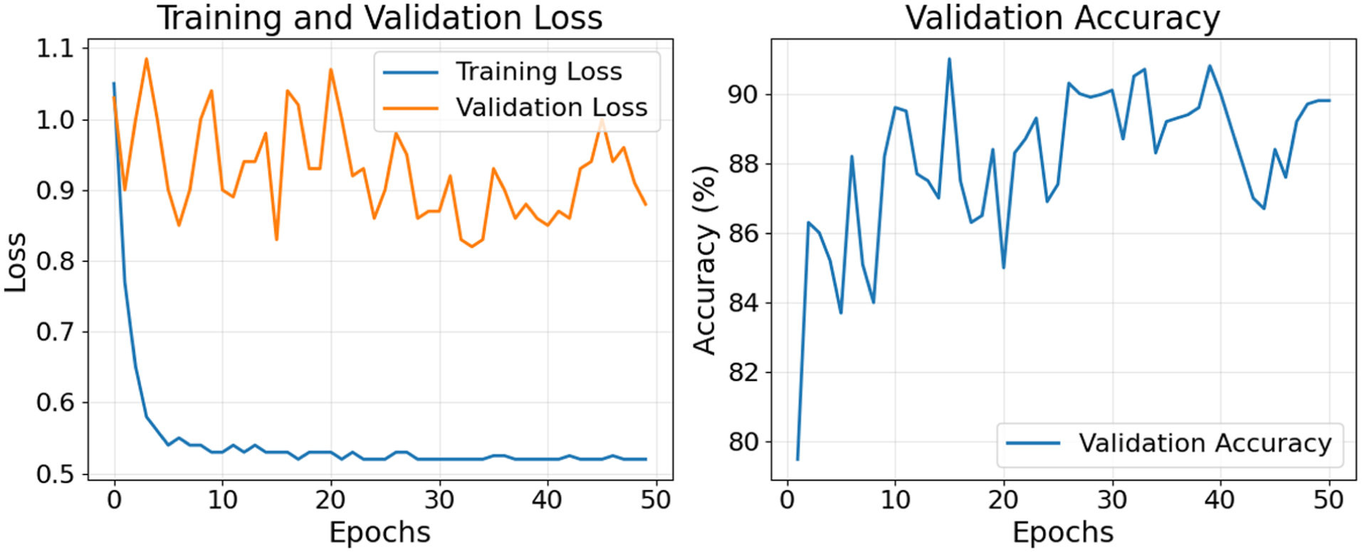
Training and validation loss (left) and validation accuracy (right) fusion method using distance map.

Figure 11.

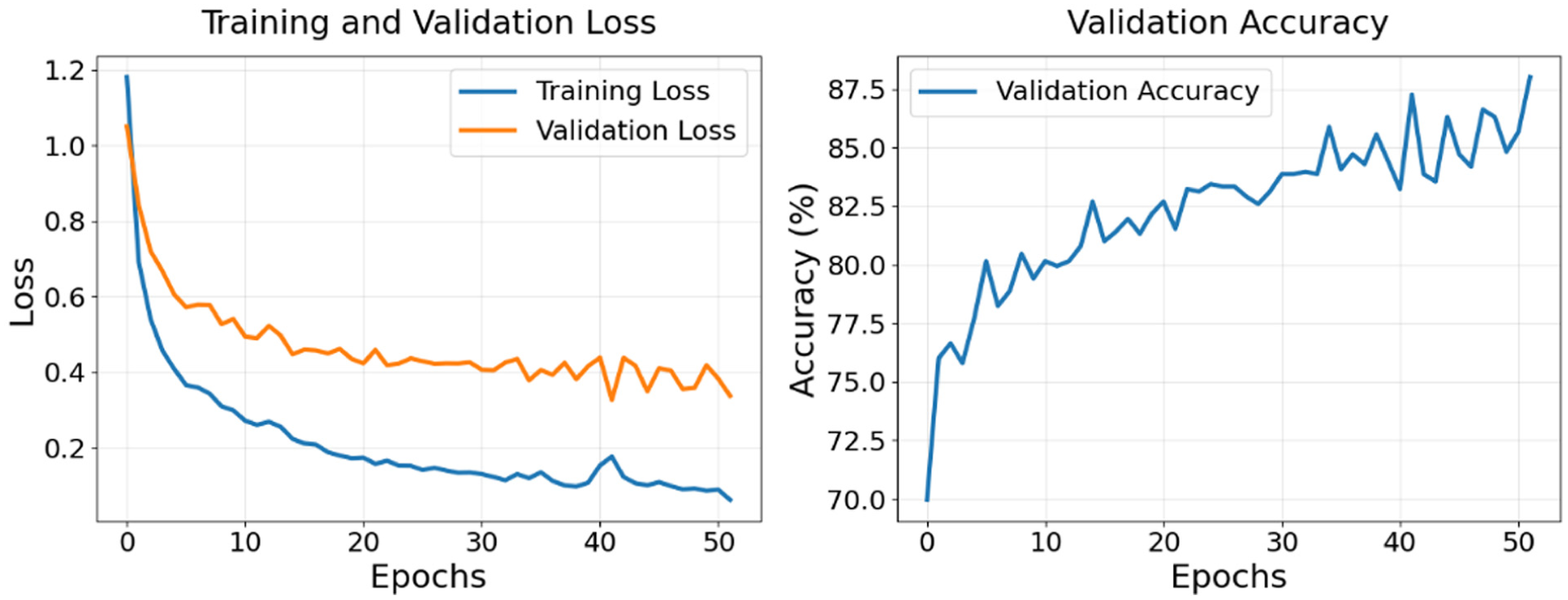
Training and validation loss plot (left) and validation accuracy plot (right) for fusion model using vehicle length.

Figure 12.

Training and validation loss plot (left) and validation accuracy plot (right) for fusion model using vehicle size.

Figure 13.

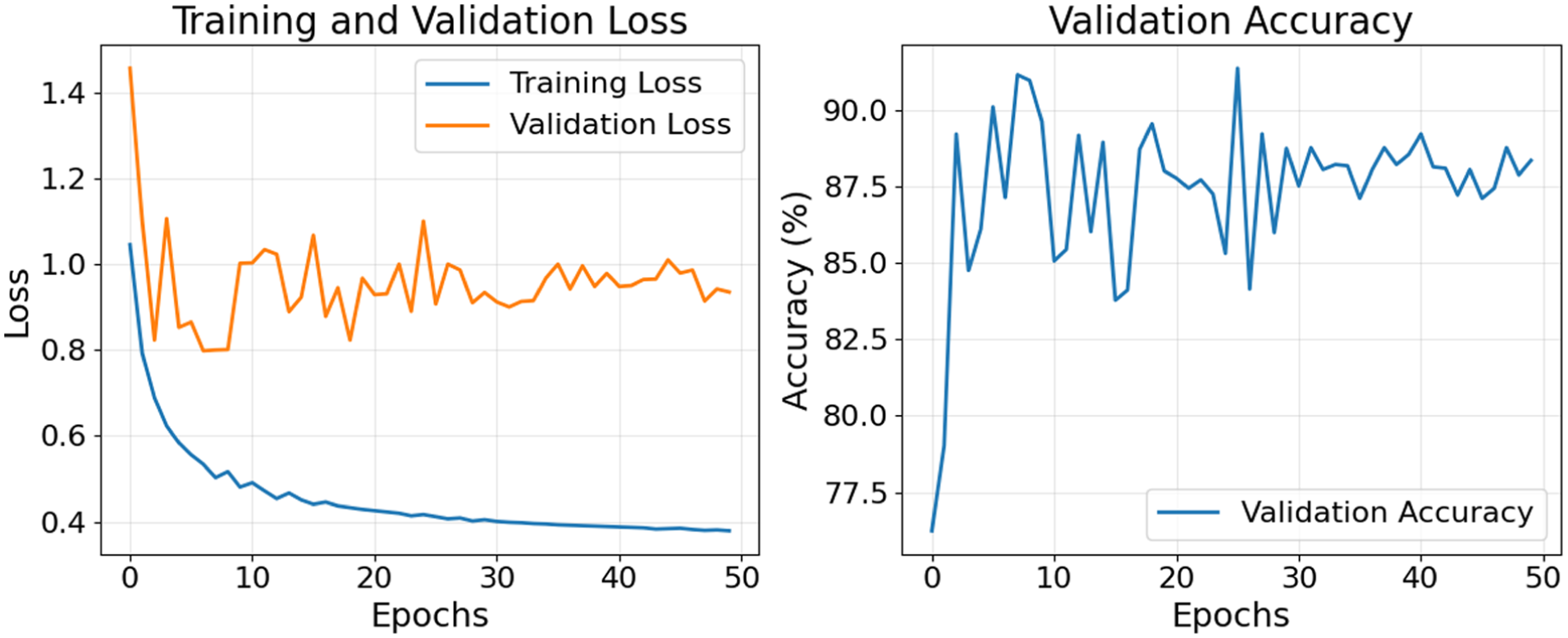
Training and validation loss plot (left) and validation accuracy plot (right) for red, green, blue, and depth (RGBD) ResNet model.

Figure 14.

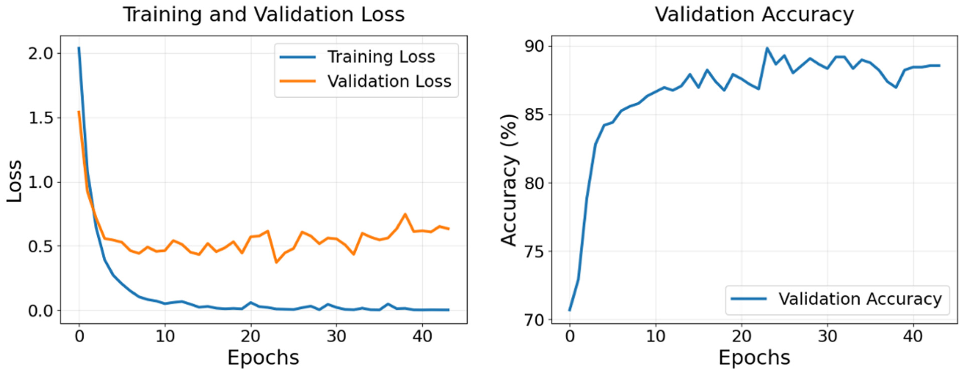
Training and validation loss plot (left) and validation accuracy plot (right) for red, green, blue (RGB) ResNet model.

Figure 15.

Training and validation loss plot (left) and validation accuracy plot (right) for PointFusion model.

Evaluation Metric

The confusion matrix is a table that helps visualize the performance of a classification model. Table 2 shows a generic confusion matrix. The true positive (TP) represents the number of correctly predicted positive instances, the false positive (FP) denotes the number of instances incorrectly predicted as positive, the true negative (TN) indicates the number of correctly predicted negative instances, and the false negative (FN) reflects the number of instances incorrectly predicted as negative.

Table 2.

Confusion Matrix

	Predicted positives	Predicted negatives
Actual positives	True positives	False negatives
Actual negatives	False positives	True negatives

The evaluation of models developed using imbalanced data sets necessitates the use of carefully selected metrics to ensure an accurate and unbiased assessment. Accuracy can be misleading when applied to imbalanced data sets, as it solely reflects the overall rate of correct predictions. Accuracy measures the ratio of correctly predicted instances to the total instances in the data set. To address this issue, precision, recall, and the F1 score are used instead. These metrics are calculated directly from the confusion matrix and do not depend on TN, focusing instead on the model’s performance on both majority and minority classes independently. Precision, as shown in Equation 4, measures the proportion of true positives among all positive predictions. Recall, as illustrated in Equation 5, measures the proportion of true positives among all actual positive instances. The F1 Score, defined in Equation 6, calculates the harmonic mean of precision and recall, providing a balanced measure that accounts for both.

Precision = \frac{TP}{TP + FP}

(4)

Recall = \frac{TP}{TP + FN}

(5)

F 1 Score = 2 \times \frac{Precision \times Recall}{Precision + Recall}

(6)

Results and Discussions

This section evaluates the performance of the fusion and baseline models. Tables 3 –8 provide a detailed summary of precision, recall, and F1 scores for each vehicle class, along with overall averages for each model. Figures 16 –21 present the confusion matrices, offering further insight into the classification performance. In addition, the models are compared based on training and inference times to assess their computational efficiency.

Table 3.

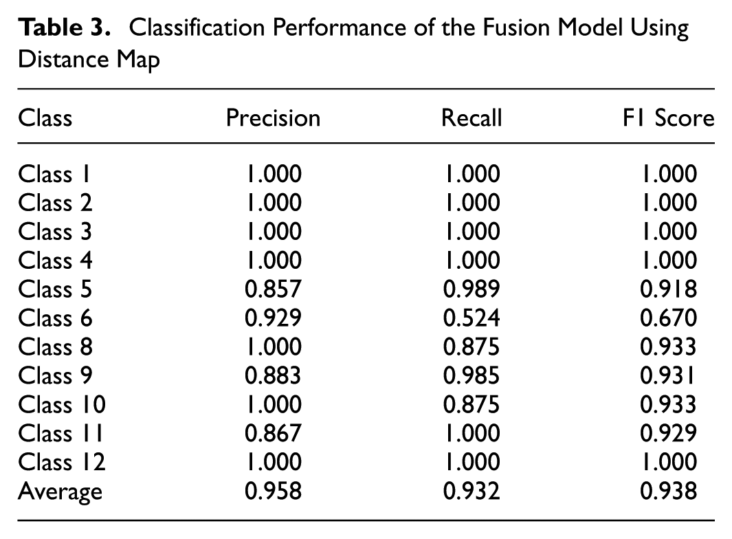
Classification Performance of the Fusion Model Using Distance Map

Class	Precision	Recall	F1 Score
Class 1	1.000	1.000	1.000
Class 2	1.000	1.000	1.000
Class 3	1.000	1.000	1.000
Class 4	1.000	1.000	1.000
Class 5	0.857	0.989	0.918
Class 6	0.929	0.524	0.670
Class 8	1.000	0.875	0.933
Class 9	0.883	0.985	0.931
Class 10	1.000	0.875	0.933
Class 11	0.867	1.000	0.929
Class 12	1.000	1.000	1.000
Average	0.958	0.932	0.938

Table 4.

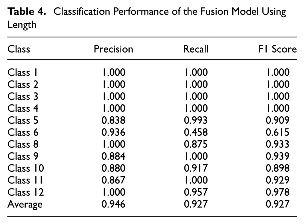
Classification Performance of the Fusion Model Using Length

Class	Precision	Recall	F1 Score
Class 1	1.000	1.000	1.000
Class 2	1.000	1.000	1.000
Class 3	1.000	1.000	1.000
Class 4	1.000	1.000	1.000
Class 5	0.838	0.993	0.909
Class 6	0.936	0.458	0.615
Class 8	1.000	0.875	0.933
Class 9	0.884	1.000	0.939
Class 10	0.880	0.917	0.898
Class 11	0.867	1.000	0.929
Class 12	1.000	0.957	0.978
Average	0.946	0.927	0.927

Table 5.

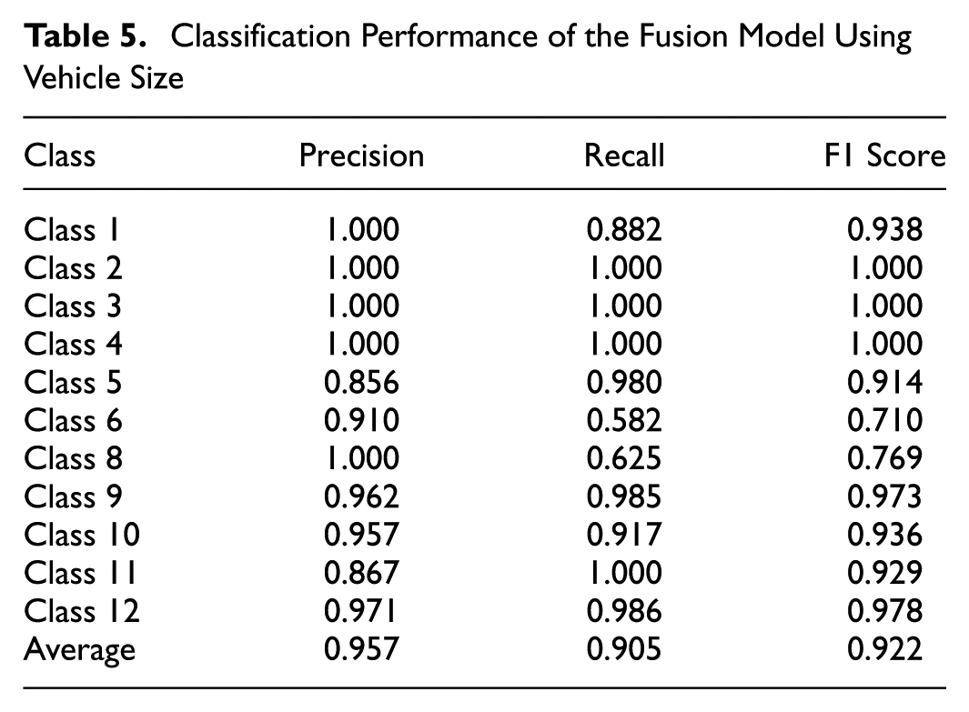
Classification Performance of the Fusion Model Using Vehicle Size

Class	Precision	Recall	F1 Score
Class 1	1.000	0.882	0.938
Class 2	1.000	1.000	1.000
Class 3	1.000	1.000	1.000
Class 4	1.000	1.000	1.000
Class 5	0.856	0.980	0.914
Class 6	0.910	0.582	0.710
Class 8	1.000	0.625	0.769
Class 9	0.962	0.985	0.973
Class 10	0.957	0.917	0.936
Class 11	0.867	1.000	0.929
Class 12	0.971	0.986	0.978
Average	0.957	0.905	0.922

Table 6.

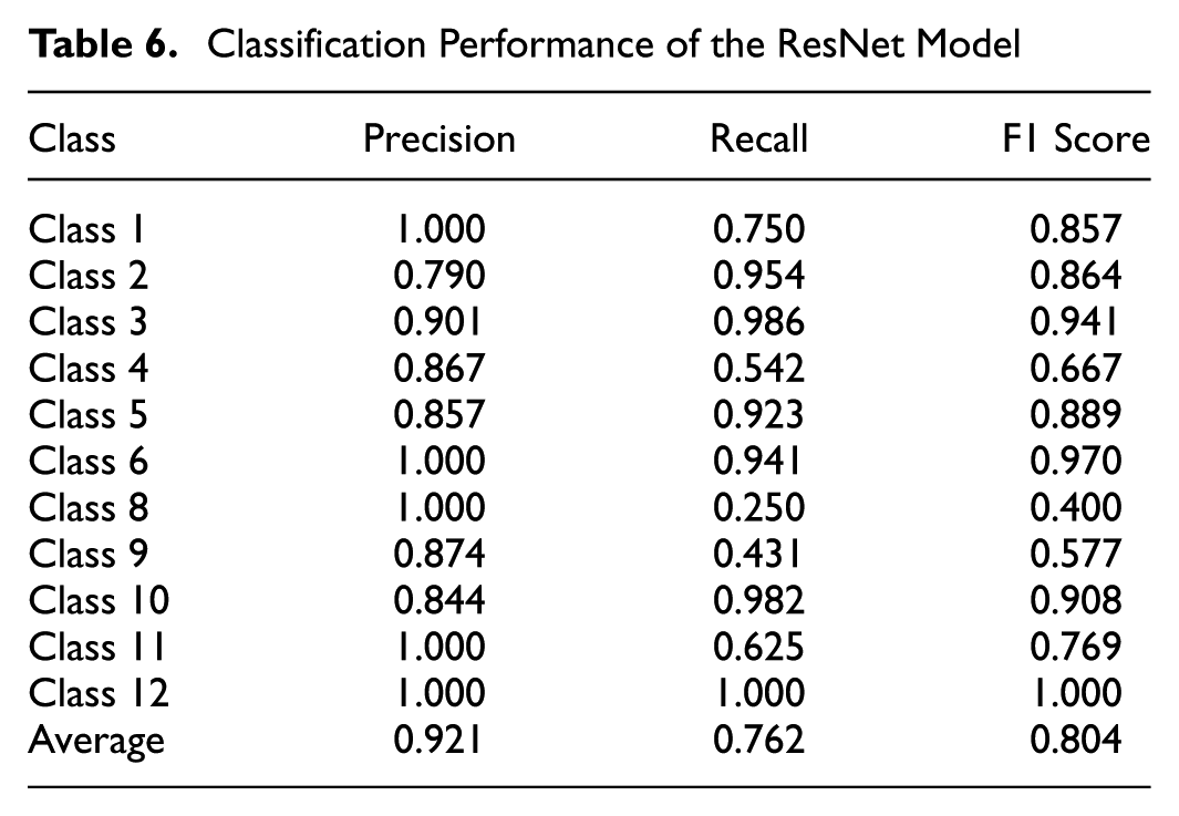
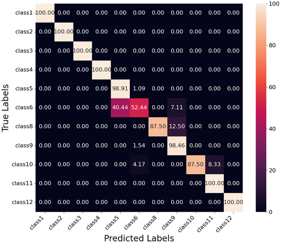
Classification Performance of the ResNet Model

Class	Precision	Recall	F1 Score
Class 1	1.000	0.750	0.857
Class 2	0.790	0.954	0.864
Class 3	0.901	0.986	0.941
Class 4	0.867	0.542	0.667
Class 5	0.857	0.923	0.889
Class 6	1.000	0.941	0.970
Class 8	1.000	0.250	0.400
Class 9	0.874	0.431	0.577
Class 10	0.844	0.982	0.908
Class 11	1.000	0.625	0.769
Class 12	1.000	1.000	1.000
Average	0.921	0.762	0.804

Table 7.

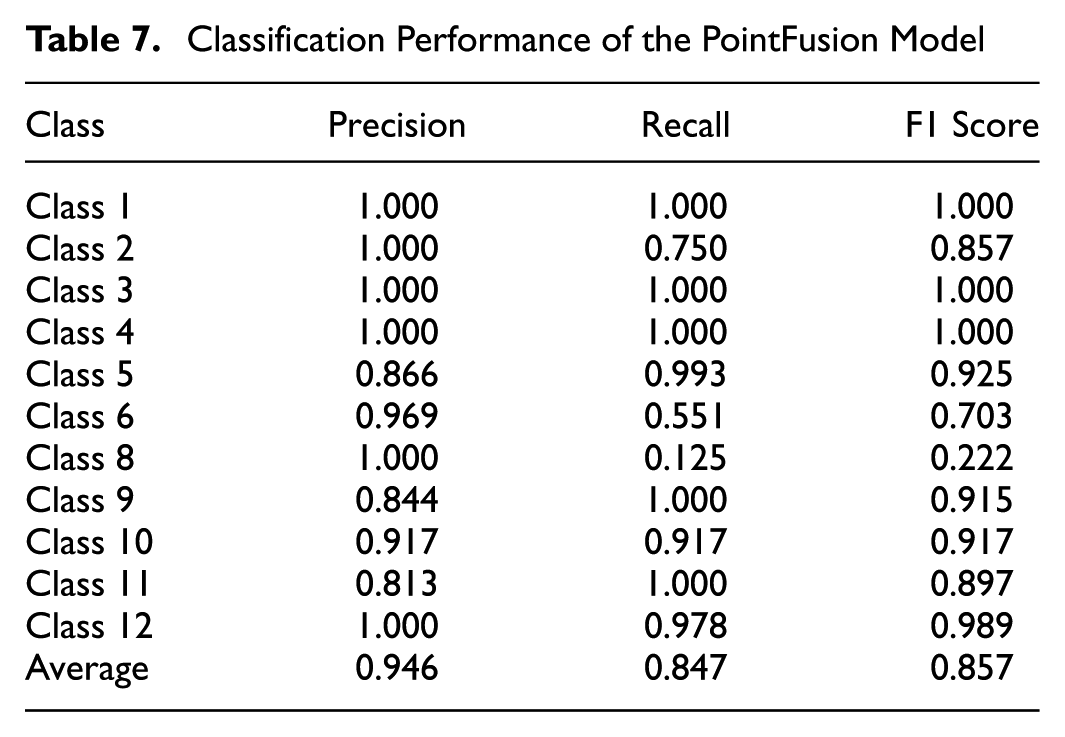
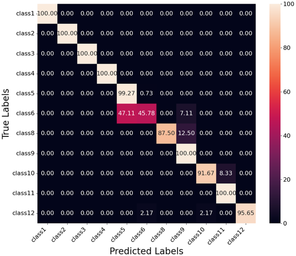
Classification Performance of the PointFusion Model

Class	Precision	Recall	F1 Score
Class 1	1.000	1.000	1.000
Class 2	1.000	0.750	0.857
Class 3	1.000	1.000	1.000
Class 4	1.000	1.000	1.000
Class 5	0.866	0.993	0.925
Class 6	0.969	0.551	0.703
Class 8	1.000	0.125	0.222
Class 9	0.844	1.000	0.915
Class 10	0.917	0.917	0.917
Class 11	0.813	1.000	0.897
Class 12	1.000	0.978	0.989
Average	0.946	0.847	0.857

Table 8.

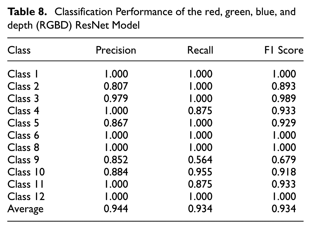
Classification Performance of the red, green, blue, and depth (RGBD) ResNet Model

Class	Precision	Recall	F1 Score
Class 1	1.000	1.000	1.000
Class 2	0.807	1.000	0.893
Class 3	0.979	1.000	0.989
Class 4	1.000	0.875	0.933
Class 5	0.867	1.000	0.929
Class 6	1.000	1.000	1.000
Class 8	1.000	1.000	1.000
Class 9	0.852	0.564	0.679
Class 10	0.884	0.955	0.918
Class 11	1.000	0.875	0.933
Class 12	1.000	1.000	1.000
Average	0.944	0.934	0.934

Figure 16.

Confusion matrix for fusion model using the distance map.

Figure 17.

Confusion matrix fusion model using vehicle length.

Figure 18.

Confusion matrix for fusion model using vehicle size.

Figure 19.

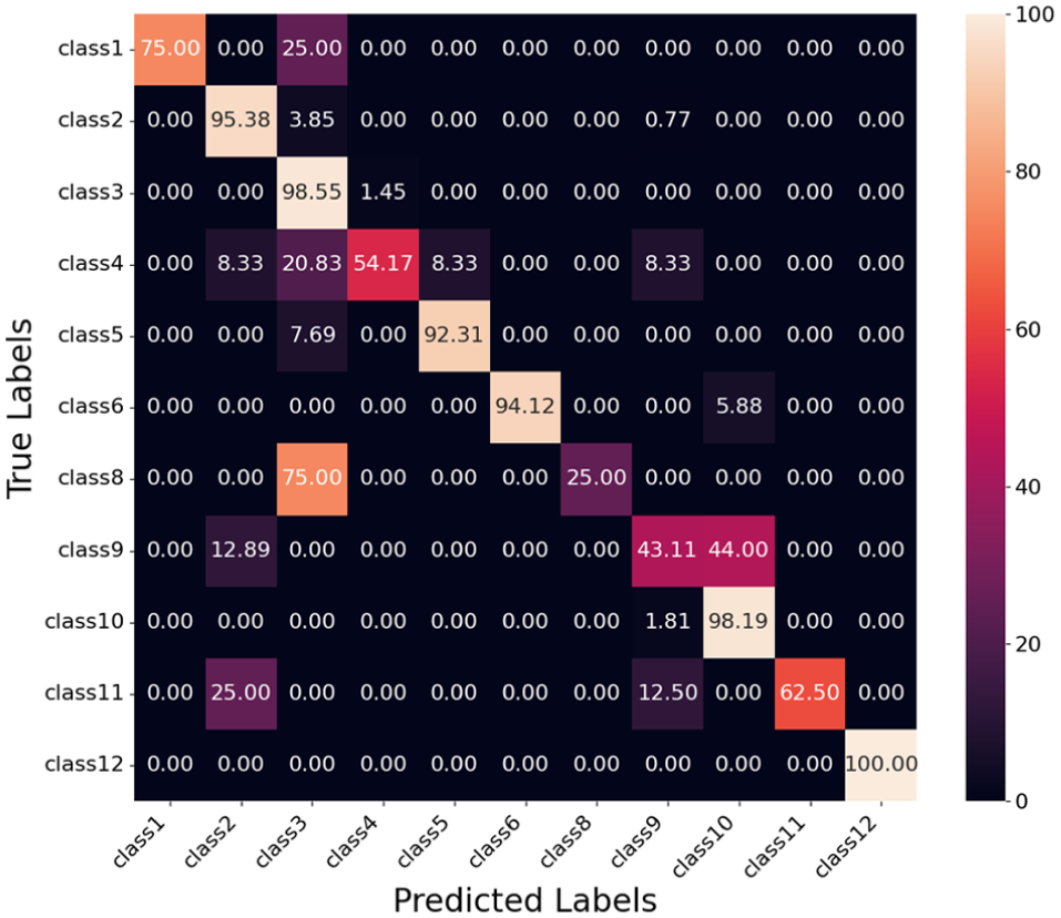
Confusion matrix for ResNet model.

Figure 20.

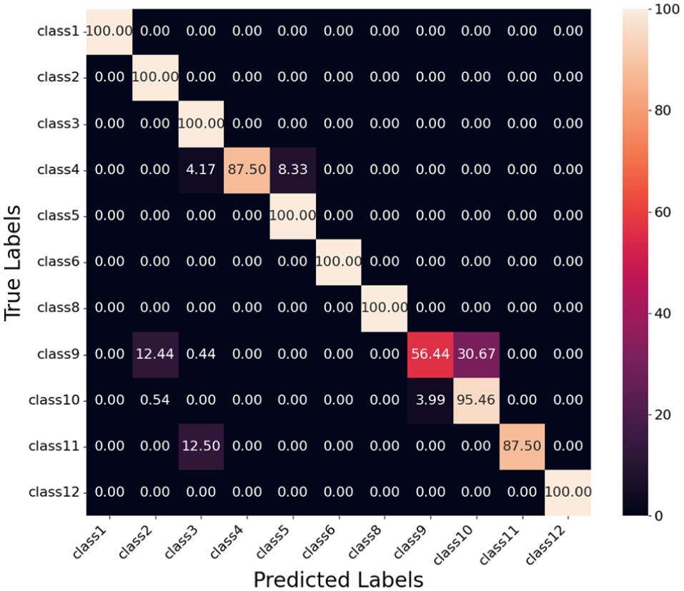
Confusion matrix for PointFusion model.

Figure 21.

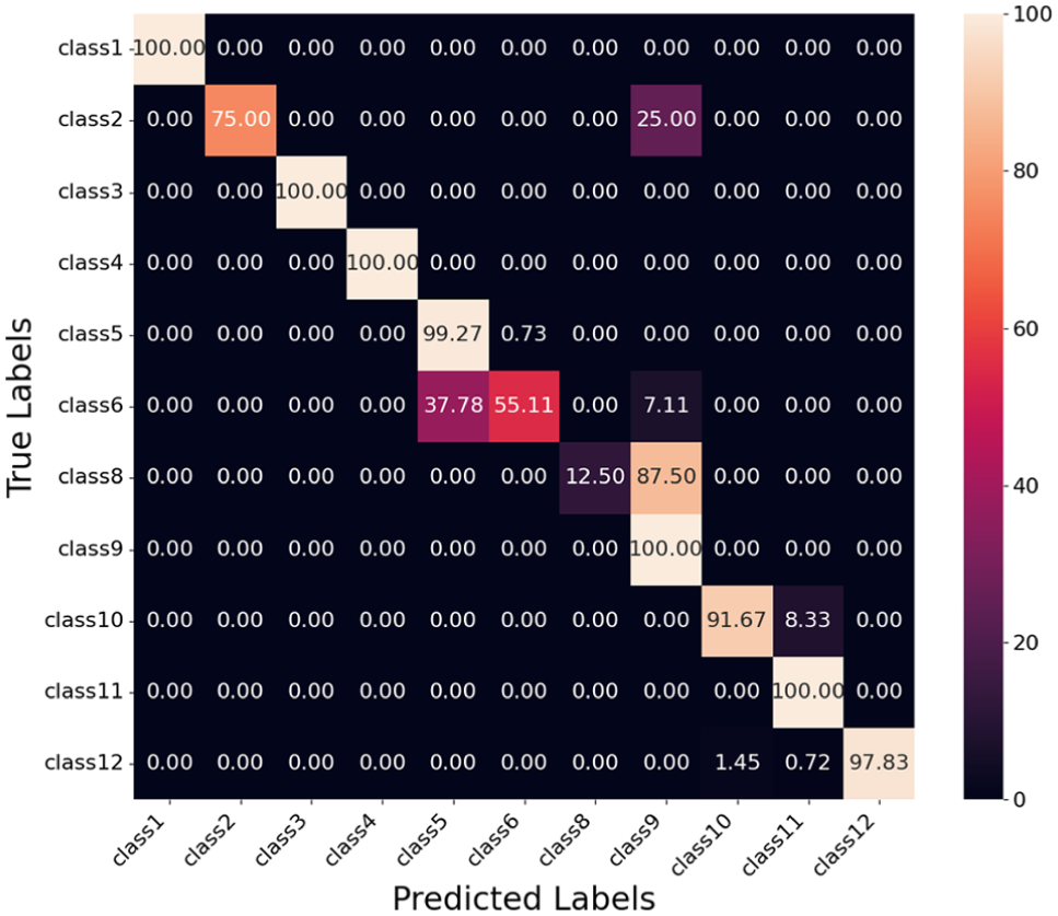
Confusion matrix for red, green, blue, and depth (RGBD) ResNet model.

Evaluation of Fusion Model Using Distance Map

Table 3 summarizes the classification performance of the fusion model using the distance map. Classes 1, 2, 3, 4, and 12 achieve perfect precision, recall, and F1 scores of 1.000, indicating that the model classifies these classes without errors when tested on our test data. Classes 8, 9, 10, and 11 also perform well, with F1 scores of 0.933, 0.931, 0.933, and 0.929, respectively.

Class 6 shows the lowest F1 score of 0.670, with a precision of 0.929 and a recall of 0.524. This indicates that while the model has high precision for Class 6, it fails to identify a significant number of true instances, as shown by the confusion matrix in Figure 16. Specifically, Class 6 is confused with Class 5 (40.44%) and Class 9 (7.11%). This confusion contributes to the high false negatives for Class 6 and explains its low recall.

Class 5 achieves an F1 score of 0.918 with a precision of 0.857 and a recall of 0.989. The relatively lower precision is a result of false positives, as a large portion of Class 6 vehicles (40.44%) are misclassified as Class 5. The high recall indicates that nearly all true Class 5 vehicles are correctly identified, with only a small fraction (1.09%) misclassified as Class 6.

Class 8 achieves high precision but has a recall of 0.875, which suggests that some true instances of Class 8 are misclassified. The confusion matrix shows these misclassifications are mainly into Class 9 (12.50%) and to a lesser extent into Class 10 (4.17%).

Overall, the model demonstrates strong performance across most classes, with an average precision, recall, and F1 score of 0.958, 0.932, and 0.938, respectively. The confusion matrix highlights areas for improvement, particularly for Class 6, where reducing misclassifications into Class 5 and Class 8 can enhance performance.

Evaluation of Fusion Model Using Length

Table 4 summarizes the classification performance of the fusion model using vehicle length. Classes 1, 2, 3, and 4 achieve perfect precision, recall, and F1 scores of 1.000, demonstrating that the model accurately classifies these classes without errors on the test data. Classes 8, 9, 10, 11, and 12 also perform well, with F1 scores of 0.933, 0.939, 0.898, 0.929, and 0.978 respectively.

Class 6 shows the lowest F1 score of 0.615, with a precision of 0.936 and a recall of 0.458. This indicates a high rate of false negatives, where many true instances of Class 6 are misclassified. The confusion matrix in Figure 17 reveals that Class 6 is predominantly confused with Class 5 (47.11% of its predictions) and Class 9 (7.11%). This explains the low recall for Class 6 and highlights the need to reduce these misclassifications.

Class 5 achieves an F1 score of 0.909 with a precision of 0.838 and a recall of 0.993. The relatively lower precision reflects false positives, as a large portion of Class 6 instances (47.11%) are misclassified as Class 5. Class 8 has high precision but a recall of 0.875, indicating that some true instances of Class 8 are misclassified as Class 9 (12.50%).

Overall, the model performs well across most classes, achieving average precision, recall, and F1 scores of 0.946, 0.927, and 0.927, respectively. The confusion matrix highlights challenges for Class 6, where reducing misclassifications of Class 6 into Class 5 and Class 9 can improve performance.

Evaluation of Fusion Model Using Size

Table 5 presents the classification performance of the fusion model using vehicle size. Classes 2, 3, and 4 achieve perfect precision, recall, and F1 scores of 1.000, demonstrating the model’s ability to classify these classes without errors. Classes 9, 10, 11, and 12 also perform well, with F1 scores of 0.973, 0.936, 0.929, and 0.978, respectively.

Class 6 shows the lowest F1 score of 0.710, with a precision of 0.910 and a recall of 0.582. The low recall indicates a high rate of false negatives, where true instances of Class 6 are being misclassified. The confusion matrix in Figure 18 shows that Class 6 is misclassified as Class 5 (40.44%) which explains its low recall. This misclassification contributes to the relatively low overall performance for this class.

Class 8 achieves an F1 score of 0.769, with a precision of 1.000 but a recall of 0.625. The lower recall suggests that many true instances of Class 8 are being misclassified, primarily into Class 12 (37.50%), as shown in the confusion matrix.

Class 5 performs well with an F1 score of 0.914, achieving a recall of 0.980 but a precision of 0.856. The lower precision reflects false positives, with many Class 6 instances (40.44%) being misclassified as Class 5.

Overall, the model achieves strong performance across most classes, with average precision, recall, and F1 scores of 0.957, 0.905, and 0.922, respectively. However, challenges remain for Class 6 and Class 8, where reducing their confusion with other classes such as Class 5 and Class 12 could further improve model performance.

Evaluation of ResNet Model

Table 6 presents the classification performance of the ResNet-152 model. Class 12 achieves the highest performance, with perfect precision, recall, and F1 scores of 1.000, demonstrating that the model classifies these classes without errors. Class 3 also performs well, achieving an F1 score of 0.941, with high precision and recall values.

Class 8 shows the lowest F1 score of 0.400, with a precision of 1.000 and a recall of 0.250. The low recall indicates that most true instances of Class 8 are misclassified, with 75% of its instances predicted as Class 3, as shown in the confusion matrix in Figure 19.

Class 9 also struggles, with an F1 score of 0.577, driven by a precision of 0.874 and a recall of 0.431. The low recall reflects high false negatives, as many instances of Class 9 are misclassified as Class 10 (44.00%) and Class 2 (12.89%).

Class 4 achieves an F1 score of 0.667, with a precision of 0.867 and a recall of 0.542. The confusion matrix shows that Class 4 is primarily confused with Class 3 (20.83%) and Class 2, 5, and 9 (8.33%), contributing to its performance limitations.

Overall, the ResNet-152 model achieves average precision, recall, and F1 scores of 0.921, 0.762, and 0.804, respectively. While it performs well for several classes, challenges remain for Class 8, where significant confusion with Class 3 occurs, and for Class 9 and Class 4, where high false negatives and misclassifications limit performance.

Evaluation of PointFusion Model

Table 7 presents the classification performance of the PointFusion model. Classes 1, 3, and 4 achieve perfect precision, recall, and F1 scores of 1.000, demonstrating that the model effectively classifies these classes without errors. Class 12 also performs well, with an F1 score of 0.989, driven by a precision of 1.000 and a recall of 0.978.

Class 8 shows the lowest F1 score of 0.222, with a precision of 1.000 but a recall of 0.125. This indicates that while the model makes no false positive predictions for Class 8, it fails to identify most true instances. The confusion matrix in Figure 20 reveals that 87.50% of Class 8 instances are misclassified as Class 9, which contributes to its low recall.

Class 6 achieves an F1 score of 0.703, with a precision of 0.969 and a recall of 0.551. The low recall reflects a significant number of false negatives, where Class 6 is predominantly misclassified as Class 5 (37.78%) and Class 9 (7.11%). This explains the performance gap for Class 6.

Class 2 also shows lower performance, with an F1 score of 0.857, driven by a recall of 0.750. This indicates that 25% of true Class 2 instances are misclassified, primarily into Class 9, as shown in the confusion matrix.

Overall, the model demonstrates good performance across most classes, with average precision, recall, and F1 scores of 0.946, 0.847, and 0.857, respectively. The challenges for Classes 6 and 8, where significant confusion occurs with other classes such as Class 5 and Class 6, highlight areas for further improvement.

Evaluation of RGBD ResNet Model

Table 8 presents the classification performance of the RGBD ResNet model. Classes 1, 6, 8, and 12 achieve perfect precision, recall, and F1 scores of 1.000, demonstrating that the model classifies these classes without errors. Classes 3, 4, and 11 also perform well, with F1 scores of 0.989, 0.933, and 0.933, respectively.

Class 9 exhibits the lowest F1 score of 0.679, with a precision of 0.852 and a recall of 0.564. The low recall indicates a significant number of false negatives, as many true instances of Class 9 are misclassified. The confusion matrix in Figure 21 shows that Class 9 is misclassified as Class 10 (30.67%) and Class 2 (12.44%). This confusion explains the performance gap for Class 9.

Class 2 achieves an F1 score of 0.893, driven by a perfect recall of 1.000 but a precision of 0.807. The lower precision reflects false positives, where Class 9 is occasionally misclassified as Class 2 (12.44%), as indicated in the confusion matrix.

Class 4 achieves an F1 score of 0.933, with a recall of 0.875 and a precision of 1.000. The lower recall suggests that some true instances of Class 4 are being misclassified as Class 5 (8.33%) and Class 3 (4.17%).

Overall, the model demonstrates strong performance across most classes, with average precision, recall, and F1 scores of 0.944, 0.934, and 0.934, respectively. The challenges for Class 9 stem from confusion with Class 10 and Class 2 highlighting areas for potential improvement.

Comparative Analysis of Models

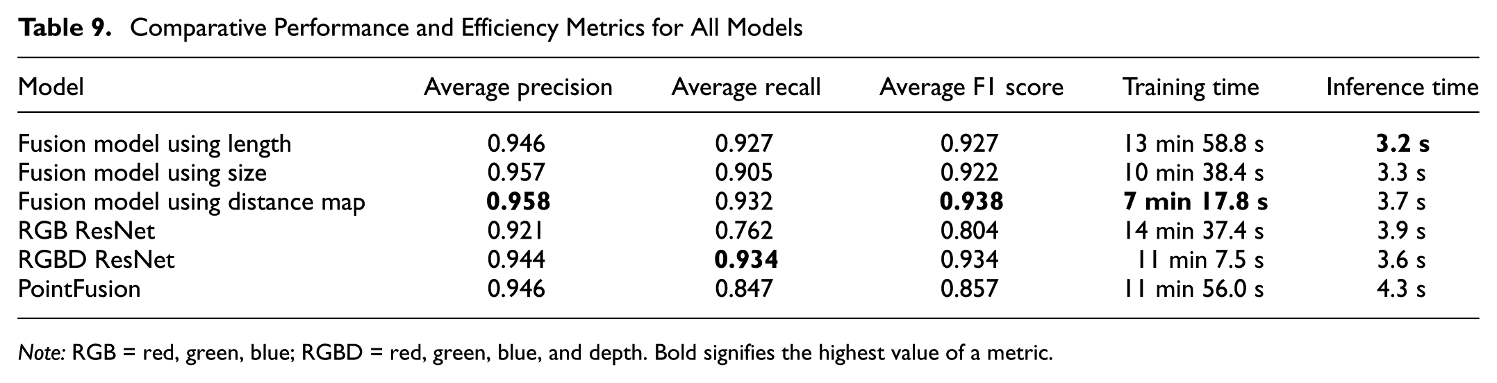
Table 9 provides a detailed summary of the models’ performance and efficiency, highlighting their respective strengths and trade-offs. Among the fusion models, the model using the distance map achieves the highest precision (0.958), and F1 score (0.938), making it the most accurate option. However, the vehicle size model offers a slightly lower F1 score of 0.922. The fusion model using vehicle length balances precision (0.946) and recall (0.927), though it has a slightly lower F1 score (0.927).

Table 9.

Comparative Performance and Efficiency Metrics for All Models

Model	Average precision	Average recall	Average F1 score	Training time	Inference time
Fusion model using length	0.946	0.927	0.927	13 min 58.8 s	3.2 s
Fusion model using size	0.957	0.905	0.922	10 min 38.4 s	3.3 s
Fusion model using distance map	0.958	0.932	0.938	7 min 17.8 s	3.7 s
RGB ResNet	0.921	0.762	0.804	14 min 37.4 s	3.9 s
RGBD ResNet	0.944	0.934	0.934	11 min 7.5 s	3.6 s
PointFusion	0.946	0.847	0.857	11 min 56.0 s	4.3 s

Note: RGB = red, green, blue; RGBD = red, green, blue, and depth. Bold signifies the highest value of a metric.

In relation to efficiency, the fusion model using the distance map is the fastest to train (7 min and 17.8 s), while the model using vehicle length achieves the shortest inference time (3.2 s). The fusion model using vehicle size combines reasonable training time and inference efficiency, offering balanced performance across metrics.

Baseline models exhibit lower precision and F1 scores overall, with the RGB ResNet achieving the lowest F1 score (0.804). However, the RGBD ResNet performs competitively, achieving the best recall (0.934) and achieving an F1 score of 0.934. Despite this, baseline models generally require longer training and inference times, with PointFusion being the slowest during inference (4.3 s).

These results highlight the superiority of the fusion models, particularly those using the distance map and vehicle length, in relation to accuracy and computational efficiency. Baseline models, while adequate, lag in performance and are less efficient under the tested conditions.

Conclusion

This research addressed the challenge of accurately classifying vehicles according to the FHWA 13-category scheme, which is essential for effective traffic management, toll collection, and transportation planning. Unlike previous studies that relied on less granular data sets or aggregated vehicle classes, this work introduces a novel methodology using a custom data set covering the 13 FHWA classes without aggregation. The approach integrates distance maps and vehicle dimensions, such as length and height, extracted from localized LiDAR point clouds with visual features from cameras. This feature-level fusion framework enhances classification granularity and accuracy, providing a practical alternative to methods that rely on aggregated data or overly complex fusion processes.

The evaluation of our proposed models demonstrates that the fusion approach using the distance map achieves the best overall performance, with an average F1 score of 0.938, recall of 0.932, and the highest precision of 0.958. This model performs exceptionally well in classes such as Classes 1, 2, 3, 4, and 12, where it achieves perfect F1 scores. Its superior performance is attributed to its ability to effectively capture spatial distribution and depth information, which provides robust geometric representations of vehicles. In contrast, the vehicle size model offers lower F1 score of 0.922. The fusion model using vehicle length demonstrates balanced performance across metrics, with precision (0.946), recall (0.927), and slightly lower F1 score of 0.927. While the RGBD ResNet performs competitively with an F1 score of 0.934, the baseline models generally show lower precision and recall overall, with RGB ResNet achieving the lowest F1 score of 0.804. The reported classification results are contingent on successful detection by YOLOv8, and the perfect F1 scores observed for certain classes reflect the characteristics of our data set and experimental setup. Performance may differ under other data conditions.

Despite the promising results, our study has certain limitations. The imbalance in the data set, particularly the underrepresentation of specific vehicle classes, may impact model performance. In addition, the omission of certain classes from the training data restricted the model’s ability to accurately classify those categories because of a lack of sufficient exposure to their features. Future work will address this limitation by incorporating the omitted classes, enhancing the model’s comprehensiveness and prediction accuracy. Another challenge was the sparseness of point clouds for vehicles at greater distances from the LiDAR sensor, which reduced the effectiveness of feature extraction. As the distance increases, fewer reflected points are available, especially for smaller vehicles, limiting the capture of key geometric details such as shape, size, and edge contours. To improve accuracy, future research should aim to expand the data set for a more balanced class distribution and develop methods to mitigate the effects of sparse point clouds for distant vehicles.

To improve LiDAR performance, manufacturers could focus on increasing laser pulse frequency and enhancing sensor resolution, which would allow for finer detail capture even at longer distances. In addition, adaptive scanning, where resolution adjusts based on object distance, could provide high detail where needed while conserving power and processing resources. For future research, integrating additional sensors such as radar can also be explored to improve model performance at a lower cost because of radar’s simpler hardware and lower processing needs. However, LiDAR remains essential for accurate vehicle classification with its high precision and 360-degree view. Radar’s durability in bad weather can complement LiDAR’s detailed resolution, supporting accurate FHWA-class classification.

Footnotes

Author Contributions

The authors confirm contribution to the paper as follows: study conception and design: Adu-Gyamfi, Zhang, Arthur; data collection: Zhang, Arthur; analysis and interpretation of results: Arthur; draft manuscript preparation: Arthur, Zhang, Adu-Gyamfi. All authors reviewed the results and approved the final version of the manuscript.

Declaration of Conflicting Interests

The authors declared no potential conflicts of interest with respect to the research, authorship, and/or publication of this article.

Funding

The authors disclosed receipt of the following financial support for the research, authorship, and/or publication of this article: The authors acknowledge financial support received for the research, authorship, and/or publication of this article from the National Science Foundation under grant award number 2045786.

ORCID iDs

Elizabeth Arthur

Linlin Zhang

Yaw Adu-Gyamfi

References

Kashuba

Vehicle Classification System: FHWA Perspective. United States Department of Transportation, Federal Highway Administration, Office of Highway Policy Information, 2000.

Traffic Monitoring Guide. Report No. FHWA-PL-022-026. Federal Highway Administration, U.S. Department of Transportation, 2022.

Coifman

Improved Velocity Estimation Using Single Loop Detectors. Transportation Research Part A: Policy and Practice, Vol. 35, No. 10, 2001, pp. 863–880.

Gholamhosseinian

Seitz

Vehicle Classification in Intelligent Transport Systems: An Overview, Methods and Software Perspective. IEEE Open Journal of Intelligent Transportation Systems, Vol. 2, 2021, pp. 173–194. https://doi.org/10.1109/OJITS.2021.3096756

Klein

L. A.

Mills

M. K.

Gibson

D. R.

Traffic Detector Handbook: Third Edition – Volume I. Publication No. FHWA-HRT-06-108. Federal Highway Administration, US Department of Transportation, McLean, VA, 2006.

Shokravi

Bakhary

Heidarrezaei

Rahimian Koloor

S. S.

Petrů

A Review on Vehicle Classification and Potential Use of Smart Vehicle-Assisted Techniques. Sensors (Basel, Switzerland), Vol. 20, No. 11, 2020, p. 3274. https://doi.org/10.3390/s20113274

Klein

L. A.

Roadside Sensors for Traffic Management. IEEE Intelligent Transportation Systems Magazine, Vol. 16, No. 4, 2024, pp. 21–44.

Premaratne

Jawad Kadhim

Blacklidge

Lee

Comprehensive Review on Vehicle Detection, Classification and Counting on Highways. Neurocomputing, Vol. 556, 2023, p. 126627. https://doi.org/10.1016/j.neucom.2023.126627

Krizhevsky

Sutskever

Hinton

G. E.

ImageNet Classification with Deep Convolutional Neural Networks. Communications of the ACM, Vol. 60, No. 6, 2017, pp. 84–90. https://doi.org/10.1145/3065386

10.

Simonyan

Zisserman

Very Deep Convolutional Networks for Large-Scale Image Recognition. arxiv.org/abs/1409.1556, 2024.

11.

Redmon

Divvala

Girshick

Farhadi

You Only Look Once: Unified, Real-Time Object Detection. IEEE Conference on Computer Vision and Pattern Recognition (CVPR), Las Vegas, NV, USA, 2016, pp. 779–788.

12.

Ren

Girshick

Sun

Faster R-CNN: Towards Real-Time Object Detection with Region Proposal Networks. IEEE Transactions on Pattern Analysis and Machine Intelligence, Vol. 39, No. 6, 2017, pp. 1137–1149. https://doi.org/10.1109/TPAMI.2016.2577031

13.

Huang

Scott

Rangarajan

Ranka

Deep Learning Based Geometric Features for Effective Truck Selection and Classification from Highway Videos. 2019 IEEE Intelligent Transportation Systems Conference (ITSC), Auckland, New Zealand, 2019, pp. 824–830.

14.

Pendse

An Overview on LiDAR for Autonomous Vehicles. Zenodo, 2024.

15.

Behley

Milioto

Stachniss

A Benchmark for Lidar-Based Panoptic Segmentation Based on Kitti. IEEE International Conference on Robotics and Automation (ICRA), Xi’an, China, 2021, pp. 13596–13603.

16.

Gothankar

Kambhamettu

Moser

Circular Hough Transform Assisted CNN Based Vehicle Axle Detection and Classification. 2019 4th International Conference on Intelligent Transportation Engineering (ICITE), Singapore, 2019, pp. 217–221.

17.

Sasongko

A. T.

Ivan Fanany

Indonesia Toll Road Vehicle Classification Using Transfer Learning with Pre-Trained Resnet Models. 2019 International Seminar on Research of Information Technology and Intelligent Systems (ISRITI), Yogyakarta, Indonesia, 2019, pp. 373–378.

18.

Liu

Huynh

D. Q.

Sun

Reynolds

Atkinson

A Vision-Based Pipeline for Vehicle Counting, Speed Estimation, and Classification. IEEE Transactions on Intelligent Transportation Systems, Vol. 22, No. 12, 2020, pp. 7547–7560.

19.

Hussain

K. F.

Afifi

Moussa

A Comprehensive Study of the Effect of Spatial Resolution and Color of Digital Images on Vehicle Classification. IEEE Transactions on Intelligent Transportation Systems, Vol. 20, No. 3, 2019, pp. 1181–1190. https://doi.org/10.1109/TITS.2018.2838117

20.

Pemila

Pongiannan

Narayanamoorthi

Sweelem

E. A.

Hendawi

Abu El-Sebah. Real Time Classification of Vehicles Using Machine Learning Algorithm on the Extensive Data set. IEEE Access, Vol. 12, 2024, pp. 98338–98351. https://doi.org/10.1109/ACCESS.2024.3417436

21.

Lee

Coifman

Side-Fire Lidar-Based Vehicle Classification. Transportation Research Record: Journal of the Transportation Research Board, 2012. 2308: 173–183.

22.

Zheng

Zhang

Tian

Automatic Vehicle Classification Using Roadside LiDAR Data. Transportation Research Record: Journal of the Transportation Research Board, 2019. 2673: 153–164.

23.

Asborno

M. I.

Burris

C. G.

Hernandez

Truck Body-Type Classification Using Single-Beam Lidar Sensors. Transportation Research Record: Journal of the Transportation Research Board, 2019. 2673: 26–40.

24.

Vatani Nezafat

Sahin

Cetin

Transfer Learning Using Deep Neural Networks for Classification of Truck Body Types Based on Side-Fire Lidar Data. Journal of Big Data Analytics in Transportation, Vol. 1, No. 1, 2019, pp. 71–82. https://doi.org/10.1007/s42421-019-00005-9

25.

Yao

Hinz

Stilla

3D Object-Based Classification for Vehicle Extraction from Airborne LiDAR Data by Combining Point Shape Information with Spatial Edge. 2010 IAPR Workshop on Pattern Recognition in Remote Sensing, Istanbul, Turkey, 2010, pp. 1–4.

26.

Dewan

Oliveira

G. L.

Burgard

Deep Semantic Classification for 3D LiDAR Data. 2017 IEEE/RSJ International Conference on Intelligent Robots and Systems (IROS), Vancouver, BC, Canada, 2017, pp. 3544–3549.

27.

Niessner

Schilling

Jutzi

Investigations on the Potential of Convolutional Neural Networks for Vehicle Classification Based on RGB and Lidar Data. ISPRS Annals of the Photogrammetry, Remote Sensing and Spatial Information Sciences, Vol. IV-1-W1, 2017, pp. 115–123. https://doi.org/10.5194/isprs-annals-IV-1-W1-115-2017

28.

Gao

Cheng

Wang

Zhao

Object Classification Using CNN-Based Fusion of Vision and LIDAR in Autonomous Vehicle Environment. IEEE Transactions on Industrial Informatics, Vol. 14, No. 9, 2018, pp. 4224–4231.

29.

Liu

Yuwen

Wan

Luo

A Lightweight Lidar-Camera Sensing Method of Obstacles Detection and Classification for Autonomous Rail Rapid Transit. IEEE Transactions on Intelligent Transportation Systems, Vol. 23, No. 12, 2022, pp. 23043–23058.

30.

S.-I.

Kang

H.-B.

Object Detection and Classification by Decision-Level Fusion for Intelligent Vehicle Systems. Sensors (Basel, Switzerland), Vol. 17, No. 1, 2017, p. 207. https://doi.org/10.3390/s17010207

31.

Lee

Han

S.-J.

Min

K.-W.

Choi

Park

C. H.

EMOS: Enhanced Moving Object Detection and Classification via Sensor Fusion and Noise Filtering. ETRI Journal, Vol. 45, No. 5, 2023, pp. 847–861. https://doi.org/10.4218/etrij.2023-0109

32.

Ultralytics. YOLOv8. https://docs.ultralytics.com/models/yolov8. Accessed Oct 22, 2023.

33.

Arthur

Muturi

Adu-Gyamfi

Training Vehicle Detection and Classification Models with Less Data: An Active Learning Approach. Transportation Research Record: Journal of the Transportation Research Board, 2024. 2678: 2146–2164.

34.

Zhang

Ren

Sun

Deep Residual Learning for Image Recognition. Proceedings of the IEEE Conference on Computer Vision and Pattern Recognition, Las Vegas, 2016, pp. 770–778.

35.

Wang

Tian

Zhang

Luo

Wang

An Improved Deep Learning Approach and Its Applications on Colonic Polyp Images Detection. BMC Medical Imaging, Vol. 20, No. 1, 2020, p. 83. https://doi.org/10.1186/s12880-020-00482-3.

Automated FHWA Vehicle Classification System via LiDAR and Camera Data Fusion

Abstract

Keywords

Introduction

Literature Review

Vision-Based Approach for Vehicle Classification

LiDAR-Based Approach for Vehicle Classification

LiDAR and Camera Fusion-Based Approach for Vehicle Classification

Data Set

Camera and LiDAR Data Collection

Data Description

Camera and LiDAR Data Synchronization

Methodology

Pretrained Yolov8

Image Feature Extraction

Distance Map Feature Extraction

Vehicle Dimension Feature Extraction

Final MLP Classifier

Baseline Models for Comparison

Experiment and Results

Training and Validation

Evaluation Metric

Results and Discussions

Evaluation of Fusion Model Using Distance Map

Evaluation of Fusion Model Using Length

Evaluation of Fusion Model Using Size

Evaluation of ResNet Model

Evaluation of PointFusion Model

Evaluation of RGBD ResNet Model

Comparative Analysis of Models

Conclusion

Footnotes

Author Contributions

Declaration of Conflicting Interests

Funding

ORCID iDs

References