Sage Journals: Discover world-class research

Abstract

The growing volume of available infrastructural monitoring data enables the development of powerful data-driven approaches to estimate infrastructure health conditions using direct measurements. This paper proposes a deep learning methodology to estimate infrastructure physical parameters, such as railway track stiffness, using drive-by vibration response signals. The proposed method employs a long short-term memory (LSTM) feature extractor accounting for temporal dependencies in the feature extraction phase, and bidirectional long short-term memory (BiLSTM) networks to leverage bidirectional temporal dependencies in both the forward and backward paths of the drive-by vibration response in the condition estimation phase. In addition, a framing approach is employed to enhance the resolution of the monitoring task to the beam level by segmenting the vibration signal into frames equal to the distance between individual beams, centering the frames over the beam nodes. The proposed LSTM-BiLSTM model offers a versatile tool for various bridge and railway infrastructure conditions monitoring using direct drive-by vibration response measurements. The results demonstrate the potential of incorporating temporal analysis in the feature extraction phase and emphasize the pivotal role of bidirectional temporal information in infrastructure health condition estimation. The proposed methodology can accurately and automatically estimate railway track stiffness and identify local stiffness reductions in the presence of noise using drive-by measurements. An illustrative case study of vehicle–track interaction simulation is used to demonstrate the performance of the proposed model, achieving maximum mean absolute percentage errors of 1.7% and 0.7% in estimating railpad and ballast stiffness, respectively.

Keywords

deep learning infrastructure inspection railway supervised learning

Infrastructure health monitoring is a fundamental component of maintaining a safe and reliable infrastructure network. Continuous monitoring over time and across the infrastructure network facilitates the infrastructure health conditions estimation, which can be used for condition-based maintenance strategies ( 1 , 2 ). This process involves assessing infrastructure damage and tracking changes in physical properties, such as modal frequencies, modal mass, modal damping, stiffness, and mode shapes ( 3 – 6 ).

In railway systems, monitoring the physical properties of infrastructure is crucial for capturing changes caused by dynamic train loading and aging track components. Track stiffness forms a primary feature determining the degradation progress of railway infrastructure ( 7 , 8 ). A sudden change in track stiffness is often related to changes in track type or associated with local damage to the ballast, substructure, and subgrade (fouled ballast, mud pumping, or hanging ties). Moreover, track stiffness is influenced by the superstructure and missing/degraded fastening components ( 9 ). Given the determining nature of track stiffness for railway condition estimation, accurate measurements of this property can significantly support maintenance decisions.

Infrastructure health conditions can be measured indirectly under both loaded and unloaded conditions using dynamic loads or external excitation forces. Two common techniques for measuring health conditions under loaded conditions are pass-by and vehicle-based (drive-by) measurements ( 10 ). Pass-by measurements are typically used for specific locations of interest and involve placing a network of accelerometers to record vibration responses at strategic points, such as bridges. These methods incur costs for sensor deployment and limit measurements to a single location. Consequently, vehicle-based measurements have become increasingly preferred since they present high-accuracy and cost-effective measurements along the entire infrastructure network.

Traditionally, infrastructure physical parameter estimation methods relied on sophisticated identification algorithms to solve inverse problems in modal parameter estimation ( 11 – 13 ). For example, Quirke et al. ( 12 ) and Zhu et al. ( 13 ) investigated track stiffness estimation using optimization techniques, namely cross-entropy ( 12 ) and adaptive regularization ( 13 ), to solve the identification optimization problem and to infer the railway track stiffness profile. However, implementing such algorithms is often computationally expensive and time-consuming ( 14 ). Furthermore, the centralized nature of parametric damage detection methods makes them infeasible for real-time damage detection applications, especially as infrastructure data continue to grow exponentially. Therefore, recent advances in machine learning, particularly deep learning techniques, offer promising alternatives for overcoming these challenges ( 15 – 22 ).

In the current paper, we further explore the estimation of infrastructure physical parameters through deep learning approaches. Railway inspection often relies on axle box acceleration (ABA) monitoring systems ( 9 , 23 , 24 ). Therefore, we develop a novel deep learning framework to estimate infrastructure health parameters using ABA measurements and demonstrate the application of our model utilizing simulated ABA signals for different track stiffness parameters. Furthermore, our methodology holds promise for broader applications in infrastructure inspections utilizing drive-by vibration measurements. For further information on drive-by infrastructure inspections, readers can refer to Hajializadeh ( 25 ).

Deep Learning in Structure Health Monitoring using Vibration Response

Deep learning techniques have increasingly gained attention in infrastructure health monitoring in recent years. The strength of these techniques to detect and locate damage directly from vibration response without any need for data preprocessing or hand-crafted feature extraction is highly promising compared to traditional vibration-based structure monitoring techniques ( 14 ). Deep learning techniques generally require a two-stage process including a damage-sensitive feature extraction through the raw acceleration signals, and processing the extracted features to assess the health state of the structure ( 14 , 26 ). Accordingly, an autoencoder-based framework has been proposed by Pathirage et al. ( 26 ) for structural damage identification, comprising two main components: dimensionality reduction and relationship learning. The first component reduces the dimensionality of the original input vector, and the second component learns the relationship between the features and the stiffness reduction. Furthermore, Huang et al. ( 27 ) proposed a convolutional neural network (CNN) framework to predict the track dynamic stiffness using the ABA measurements in real-time, including a comparison of the performance between the standard CNN and dilated CNN algorithms. Both models performed well considering their accuracy, with the dilated CNN requiring less computation time in both the training and deployment processes. While the CNN effectively captures relevant information within a neighborhood of samples, it often struggles to learn long-term dependencies in sequential datasets, which is relevant for railway track parameter estimation over a long period of data. To address this, Le-Xuan et al. ( 28 ) proposed a 1DCNN-LSTM-ResNet architecture to identify structural damages based on time-dependent data. The model employs a one-dimensional CNN (1DCNN) for feature extraction, long short-term memory (LSTM) for recognizing long-term dependencies, and ResNet to counteract the vanishing gradient problem during deep network training. The proposed architecture outperformed the 1DCNN, LSTM, and their combination in diagnosing the damage states of the Z24 bridge located in the Bern district near Solothurn, Switzerland. In Locke et al. ( 29 ), the frequency spectrum of simulated acceleration signals was utilized to develop and train a 1DCNN deep learning algorithm. The paper ( 29 ) showed that a one-dimensional (1D) variant of VGG convolutional networks can detect bridge damage across a range of real-world noise signals. In fact, CNNs are designed to efficiently extract spatial and hierarchical features from data, making them particularly effective for inputs like vibration response signals. The process of applying filters and pooling in a CNN helps capture essential features while reducing spatial dimensions, which not only enhances computational efficiency but also preserves critical information ( 29 ).

Moreover, structure health monitoring has been addressed with anomaly detection approaches. Jie et al. ( 30 ) and Sharma and Sen ( 31 ) developed LSTM-based anomaly detection frameworks to identify vibration sequence anomalies in subway tracks and bridges, respectively. The LSTM model was trained only on normal sequences, and the anomaly score was estimated via the reconstruction error between the model input sequence and output sequence. The input sequence was identified as an anomaly sequence through comparison with the anomaly threshold value. Although the anomaly detection approach is highly applicable when there are limited available data for malfunction conditions, since the model’s training process is biased toward normal cases, it may not generalize well to abnormal situations.

Contributions of this Paper

In this paper, we propose an innovative model architecture, namely bidirectional long short-term memory (BiLSTM) networks, to estimate infrastructure physical parameters using vehicle-based vibration responses. This work makes the following contributions with respect to the state-of-the-art. Firstly, our work highlights the pivotal role of the bidirectional temporal dependencies in both the forward and backward paths of the vibration response of the infrastructure. The idea stems from each sequence of vibration responses being influenced by both the forward and backward paths of the infrastructure’s vibration response. By using BiLSTM networks, we can effectively capture and integrate these temporal relations, leading to more accurate infrastructural health condition estimations. Secondly, we enhance the infrastructure monitoring resolution to beam nodes using the proposed framing approach to leverage accurate vibration signal positions. This framing approach segmentizes the vibration response within bearing spans over the beam nodes, which facilitates localized condition estimation at individual beam resolutions. Thirdly, the methodology employs a novel feature extraction method based on a LSTM layer and proposes the potential of incorporating temporal relations even at the feature extraction level. Our model exhibits excellent performance in a case study focusing on railway track segments, demonstrating accurate estimation of railpad and ballast stiffness, and identifying local stiffness reductions in a noisy environment.

Preliminaries

LSTM Cell

LSTM was introduced as an enhancement over traditional recurrent neural networks (RNNs) for long-term dependency ( 32 ). The LSTM network captures temporal dependencies with additional memory cells. A LSTM memory cell controls the flow of information and handles the memory efficiently using three types of gates: input, forget, and output gates, as shown in Figure 1. Given a time-series input $x = (x_{1}, \dots, x_{T})$ , where T represents the last time step t, the LSTM updates the hidden state $h_{t}$ using current input information $x_{t}$ , hidden prior information state $h_{t - 1}$ , input gate $g_{i, t}$ , forget gate $g_{f, t}$ , output gate $g_{o, t}$ , and a memory cell $c_{t}$ . The mathematical expression for a forward pass of a LSTM unit can be defined as follows:

g_{i, t} = σ (W_{x i} x_{t} + W_{h i} h_{t - 1} + b_{i})

(1)

g_{f, t} = σ (W_{x f} x_{t} + W_{h f} h_{t - 1} + b_{f})

(2)

g_{o, t} = σ (W_{x o} x_{t} + W_{h o} h_{t - 1} + b_{o})

(3)

{\tilde{c}}_{t} = \tanh (W_{x \tilde{c}} x_{t} + W_{h \tilde{c}} h_{t - 1} + b_{\tilde{c}})

(4)

c_{t} = g_{i, t} \otimes {\tilde{c}}_{t} + g_{f, t} \otimes c_{t - 1}

(5)

h_{t} = g_{o, t} \otimes \tanh (c_{t})

(6)

y_{t} = σ (W_{y} h_{t} + b_{y})

(7)

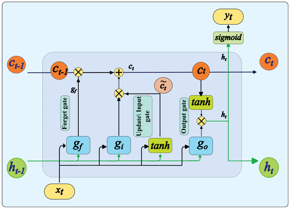
where the $notation \otimes$ is an operator for point-wise multiplication of vectors, $φ$ and $σ$ are the $\tanh$ and sigmoid activation functions, respectively, and W and b are respectively weight matrices and bias parameters for each LSTM cell. Moreover, ${\tilde{c}}_{t}$ denotes the cell input activation vector and $c_{t}$ and $c_{t - 1}$ denote the cell state values at time steps t and $t - 1$ respectively. The input gate $g_{i, t}$ determines the cell state that needs to be updated, the forget gate $g_{f, t}$ decides what information should be overlooked, and the output gate $g_{o, t}$ determines which part of the cell state should be exported.

Figure 1.

Long short-term memory (LSTM) cell. The fundamental components of a LSTM cell are the forget, input, and output gates, the updating cell state, and the hidden state.

A cell state $c_{t}$ consists of two components: (i) $g_{i, t} \otimes {\tilde{c}}_{t}$ , which includes the relevant information from ${\tilde{c}}_{t}$ through $g_{i, t}$ ; and (ii) $g_{f, t} \otimes c_{t - 1}$ , which forgets the less-relevant information from $c_{t - 1}$ . In the final step, the hidden state $h_{t}$ is employed to predict $y_{t}$ at each time step. The entire network is parameterized with the weight matrices and bias parameters and is learned during backpropagation.

1D Convolutional Neural Networks

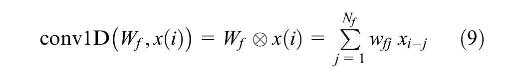
1DCNNs are recognized in deep learning for their proficiency in handling local relationships in sequential and time-series data. A basic 1DCNN comprises several 1D filters in the 1DCNN layer and 1D pooling layers to capture the spatial patterns by applying the convolution operation. During this process, filters slide across time steps, creating feature maps that capture detailed and abstract representations of the data’s patterns. Feature maps are essentially the outputs of the convolution process, depicting different aspects of the input data. Moreover, pooling layers complement this by downsampling the outcome of the convolution process, effectively emphasizing important features while reducing computational load. Max-pooling or average pooling layers are commonly used to summarize the feature maps by reducing their spatial dimensions and highlighting salient features in the process.

The formula of one typical convolutional layer is as follows:

\begin{matrix} h_{f} = conv 1 D (W_{f}, x) + b_{f} \end{matrix}

(8)

where $h_{f}$ , $W_{f}$ , and $b_{f}$ are respectively the output vector, weight matrices, and bias parameter of the filter f, while x is the input vector and $conv 1 D$ is the 1D convolution operator whose $i^{th}$ output is calculated by the following formula:

\begin{matrix} conv 1 D (W_{f}, x (i)) = W_{f} \otimes x (i) = \sum_{j = 1}^{N_{f}} w_{fj} x_{i - j} \end{matrix}

(9)

where $N_{f}$ is the length of the filter f and $W_{fj}$ is the $j^{th}$ element of matrices $W_{f}$ .

Methodology

Problem Statement

Infrastructure health condition estimation using vehicle-based vibration response requires spatial and temporal analysis of the vibration signals. We approach the drive-by vibration response as a sequence of vibration signals associated with the sequence of beams and their physical properties. Our framing approach segmentizes the vibration response signal with the spans, equal to the distances between individual beams, and located at the beam nodes. These bearing spans are associated with the lengths where, under normal conditions, a beam node bears a relative load between the beam nodes. By segmenting the vibration signal over the bearing spans at the beam nodes, we leverage domain knowledge about the position of beams and the vibration signal, enhancing the resolution of infrastructure health monitoring at the beam level. For instance, in the case of railway track monitoring, the vibration signal is framed for each sleeper as a beam node, with the length of the bearing span equal to the distance between individual sleepers, centered at each sleeper position. Consequently, the sequential model can estimate health conditions in a sequential manner at the resolution of individual sleepers.

The proposed approach involves a multi-level sequential data analysis. Firstly, the lower-level network performs the feature extraction task over the vibration response segments. Secondly, the upper-level BiLSTM network takes the extracted features to estimate the health conditions over the sequence of beams. The two steps are performed in sequence with an end-to-end approach. This eliminates defining hand-crafted features, which may require expert knowledge and limits a fully automated analysis. The hidden layers of the deep learning network are learned through the backpropagation process corresponding to the last layer of the network. The initial layers may extract more meaningful features, such as sharp changes in the input signal, and the deeper layers may extract more abstract and high-level features. The Lower Level-Bearing Span Feature Extractor section below discusses the lower-level bearing span feature extraction methods, followed by the Upper-Level BiLSTM Networks section, which discusses upper-level BiLSTM networks for the estimation of health conditions.

Lower-Level Bearing Span Feature Extractor

1DCNN

The idea behind using the 1DCNN in the feature extraction phase is to leverage the strength of the 1DCNN in capturing local relationships in this phase. The 1DCNN can provide features for the upper-level model based on local relations within the input signal. The 1DCNN architecture used in this paper consists of convolutional and max-pooling layers, followed by a flattening layer and a fully connected layer, which forms the output layer of the feature extraction process. The hyperparameters of the feature extraction network include the number of convolutional layers, the number of filters per layer, the filter lengths, and the size of the dense layer, which represents the latent space of the feature extractor.

To optimize the model architecture, grid search is employed for hyperparameter tuning. The resulting network processes high-frequency time-domain signals of length 8660 and applies three convolutional and max-pooling layers of 32, 64, and 128 filters with a filter length of 8. The output of the convolutional layers is activated by a rectified linear unit (ReLU) function to increase the nonlinear expression of networks. In max-pooling layers, the pool size is $1 \times 2$ and the stride is two. The CNN’s output is flattened and passed through a dense layer with 128 units to generate the final feature vector for the subsequent health condition estimator.

While 1DCNNs emphasize the local patterns in the input sequence, they can be less efficient in capturing temporal dependencies, especially when the filter size is not sufficiently large. However, recurrent architectures, such as LSTMs, effectively address this challenge by capturing temporal information using their cell memory. Therefore, we also investigate the performance of a LSTM feature extractor in the feature extraction phase.

LSTM

The LSTM feature extractor captures temporal relationships within the input sequence. While the vibration signal exhibits long-term temporal relations in the upper-level beam-to-beam context, temporal relations can be captured during the feature extraction phase using a LSTM feature extraction layer. The feature extraction network consists of a single LSTM layer, which processes frames of vibration signals and outputs the hidden state of the last time step as the extracted feature for each frame. This hidden state serves as the feature vector for the subsequent BiLSTM health condition estimator networks. The hyperparameters of the LSTM feature extractor networks include the number of LSTM layers and LSTM units per layer. Grid search tuning identified an optimal architecture with one LSTM layer containing 128 LSTM units.

Upper-Level BiLSTM Networks

After extracting features from the bearing span frames in the lower-level analysis, the output is fed into BiLSTM networks at the upper level to capture the long-term temporal relations between sequences of beams. This approach is based on the physics of vehicle-based vibration response signals, where sequences are related to both the forward and backward paths of the sequence. For example, when there is a defect in one of the beams in a sequence, it is reflected not only in the forward path of the drive-by vibration signal but also in the backward path. Therefore, we propose using BiLSTM networks consisting of two stacked BiLSTM layers with 128 and 64 units, respectively. The outputs of these layers are concatenated and passed to the subsequent layers. The bidirectional information is then fed into a fully connected network with two dense layers consisting of 64 and 2 units, respectively, to produce the final output vector. The key hyperparameters include the number of BiLSTM layers, the units in each layer, and the number of dense layers. A schematic view of the LSTM-BiLSTM model architecture is provided in Figure 2.

Figure 2.

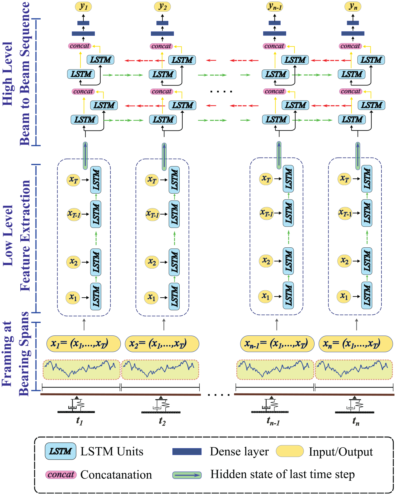
Model architecture of the proposed long short-term memory (LSTM)-bidirectional LSTM model.

Illustrative Case Study of Railway Track Monitoring

Railway track stiffness is a key indicator of track health and is widely used to monitor infrastructure conditions. It is influenced by various parameters associated with track components, including the rail, sleepers, fastening systems, ballast, and track substructure. Among these, ballast stiffness primarily determines overall track stiffness; however, fastening systems—comprising bolts, clamps, and rail pads—also play a significant role. In this study, track stiffness is characterized using railpad and ballast stiffness parameters, represented as the vector $k = [k_{p}, k_{b}]^{T}$ . The influence of fastening components, such as bolts and clamps, is considered through the rail pad stiffness parameter. The primary objective of this analysis is to estimate track stiffness parameters based on observed ABA vibration responses.

Data

Data used in the illustrative case study are based on the finite-element simulation model proposed by Shen et al. ( 9 ) and are available online ( 33 ). In this model, the rail and sleepers are meshed using Timoshenko beam elements, while the ballast and railpads are represented as discrete spring–damper pairs. Clamps and bolts are not explicitly modeled; instead, their stiffness is incorporated into the railpad stiffness, a widely accepted simplification in railway track modeling ( 9 , 34 , 35 ). The wheel is simplified as a rigid mass, and the wheel–rail contact is modeled using a Hertzian spring. In real-world railway networks, different track types exist because of variations in rail types, fastening systems, sleeper types, and sleeper spacing, which the current simulation may be limited in accounting for ( 9 ). Figure 3 illustrates a schematic view of the finite-element model for a 10-sleeper track segment alongside the corresponding framing approach for the vibration response signal. We use this model to simulate ABA measurements at an operational speed of 65 km/h by considering floating stiffness reduction and additive white Gaussian noise scenarios.

Figure 3.

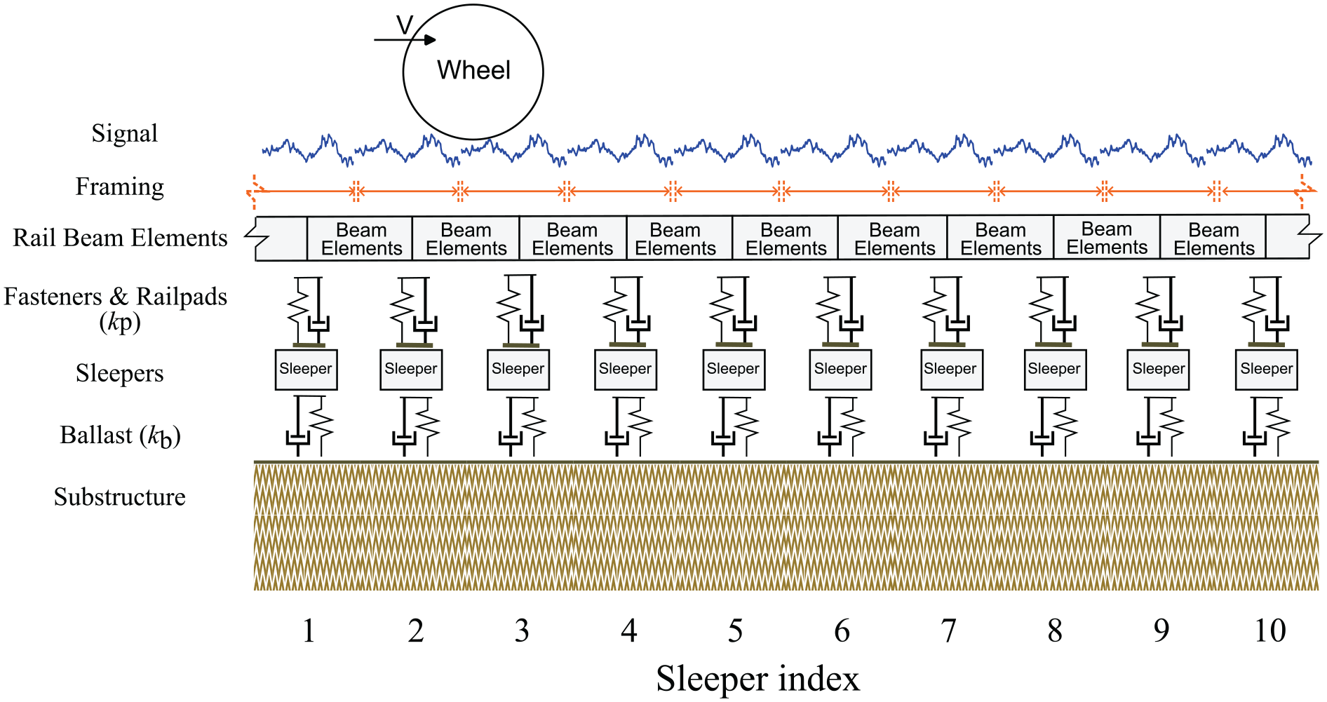
The layout of the 10-sleeper track segment.

The dataset includes cases of both constant track stiffness and local variations in track stiffness, caused by changes in railpad and ballast stiffness. The constant track stiffness scenario represents normal railway track conditions, where stiffness remains uniform along the track. To simulate this scenario, ballast and railpad stiffness values are randomly sampled from the stiffness range set R1 in Table 1, following a uniform distribution. The stiffness reduction is considered in two scenarios: reduction in one sleeper and reduction in three sleepers within a 10-sleeper segment at random locations. The stiffness reduction in one sleeper simulates a defect such as a hanging sleeper, where an unsupported sleeper hangs within the railway segment, causing a local reduction in track stiffness at that sleeper. The stiffness reduction in three sleepers simulates a scenario where a reduction in substructure support over a wider length leads to reduced stiffness in multiple sleepers ( 9 ). The stiffness of the railpad and ballast are simultaneously reduced to the stiffness range set R2 in Table 1, using a random variable with uniform distribution. The stiffness range set R2 represents multiple faults with varying severities, including degraded or missing railroads or local reductions in ballast stiffness ( 9 ). The lower bound of the range set R2 indicates more harsh scenarios of component degradation, such as ballast crushing or hanging sleepers ( 36 ). The random locations of stiffness reduction within the track segment prevent biases in the spatial distribution of defects, making the simulations more representative of real-world scenarios.

Table 1.

Range of Parameter Values Used for Railpad and Ballast Stiffness

Range sets (range of values of the model’s parameters)	$k_{p} (N / m)$	$k_{b} (N / m)$
R1	$1.5 \cdot 10^{8}$ – $3 \cdot 10^{8}$	$1.6 \cdot 10^{7}$ – $2.2 \cdot 10^{7}$
R2	$0.1 \cdot 10^{8}$ – $1.5 \cdot 10^{8}$	$0.4 \cdot 10^{7}$ – $1.6 \cdot 10^{7}$

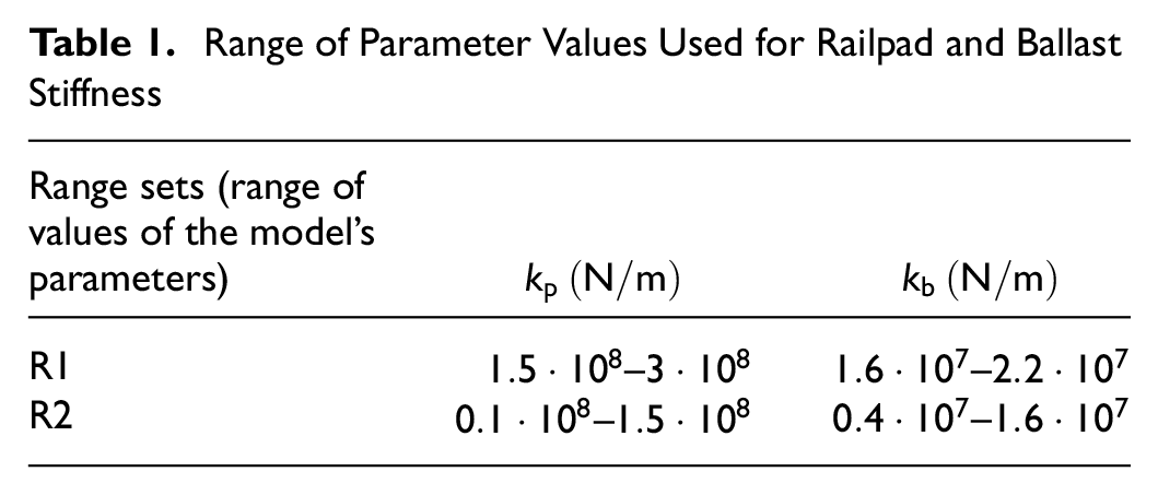
Noise is an inherent aspect of signal measurement, present even in data acquired from highly accurate sensors. Drive-by vibration responses are also affected by measurement noise caused by environmental and vehicle-induced noise. Therefore, an additive white Gaussian noise $~ N (0, σ^{2})$ is added to the ABA signal, where $σ$ is the standard deviation of the measurement noise. A noise-to-signal ratio of 15% is used, with a variance equal to 15% of the ABA signal power. The additive Gaussian noise in the ABA signal is considered to simulate real-world measurement conditions and evaluate the performance of the proposed model under such conditions ( 37 , 38 ). Each of the noise-free and noise-added scenarios consists of 15000 records of 10-sleeper track segments, and the datasets are split into training, validation, and test sets, with 60%, 20%, and 20% of the total records, respectively.

Results

In this section, we present the performance of the proposed LSTM-BiLSTM networks in estimating track stiffness using railway ABA measurements. For comparison, we also consider three other model architectures: 1DCNN-LSTM, LSTM-LSTM, and 1DCNN-BiLSTM.

During the training and validation process, the data is split into training and validation sets. Figure 4 shows the training and validation loss convergence of the four models (CNN-LSTM, LSTM-LSTM, CNN-BiLSTM, and LSTM-BiLSTM) on the noise-added datasets, demonstrating the loss convergence versus the number of epochs on a logarithmic scale. The figure indicates that the LSTM-BiLSTM architecture achieves the lowest training and validation loss compared to the other models. Furthermore, the figure shows no evidence of overfitting in the training process. The validation set is used to fine-tune the hyperparameters of the models using a grid search method. The performance of the selected fine-tuned models is then evaluated on the test set, with the results presented in Table 2. Two evaluation metrics, the mean absolute percentage error (MAPE) and root mean square error (RMSE), are used to compare the accuracy of the models in stiffness estimation. The MAPE measures the average absolute percentage difference between predicted and actual values, while the RMSE measures the square root of the average squared differences between predicted and actual values.

Figure 4.

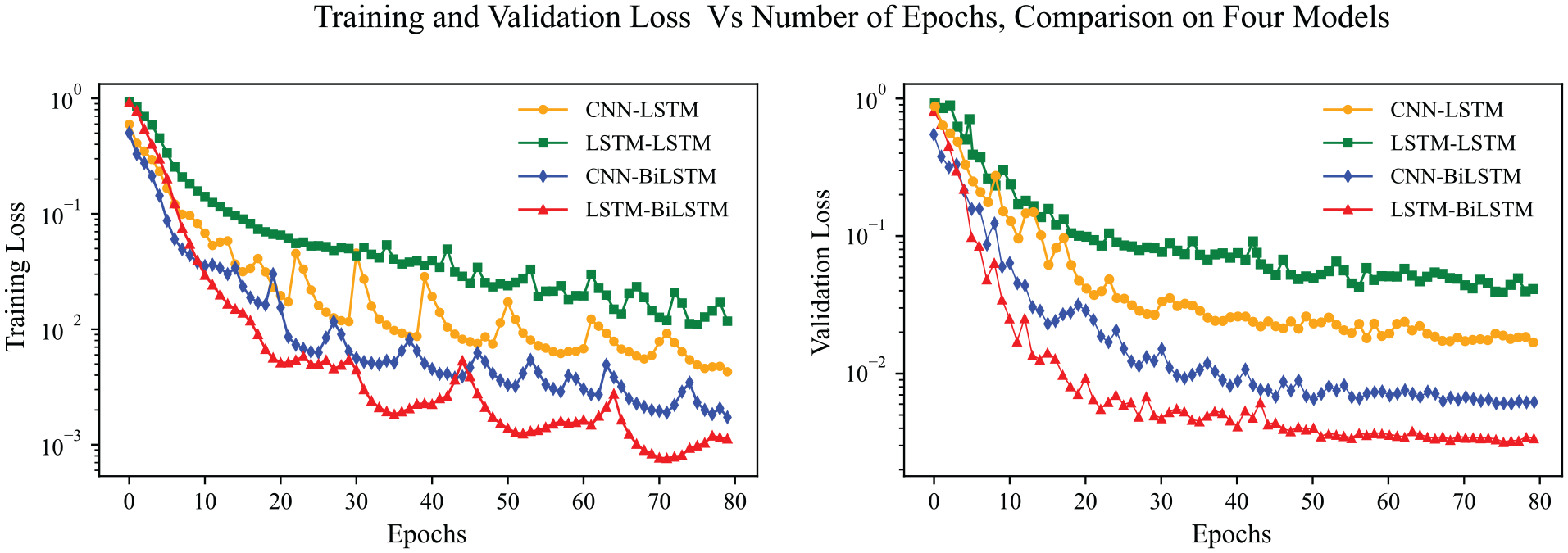
Training and validation loss convergence for the noisy dataset.

Table 2.

Models Estimation Accuracy Performance on the Test Set in Noise-Free and (15%) Noisy Datasets

Models	Noise-free dataset					Noisy dataset
	$k_{p}$		$k_{b}$		Overall	$k_{p}$		$k_{b}$		Overall
	RMSE	MAPE	RMSE	MAPE	MAPE	RMSE	MAPE	RMSE	MAPE	MAPE
CNN-LSTM	3.68	2.29%	0.18	1.04%	1.66%	8.59	5.15%	0.45	2.20%	3.60%
LSTM-LSTM	4.36	2.71%	0.25	1.12%	1.92%	11.71	6.41%	0.51	2.59%	4.50%
CNN-BiLSTM	2.81	1.76%	0.14	0.74%	1.25%	6.39	3.90%	0.38	1.57%	2.77%
LSTM-BiLSTM	0.82	0.61%	0.06	0.35%	0.47%	2.72	1.70%	0.13	0.70%	1.20%

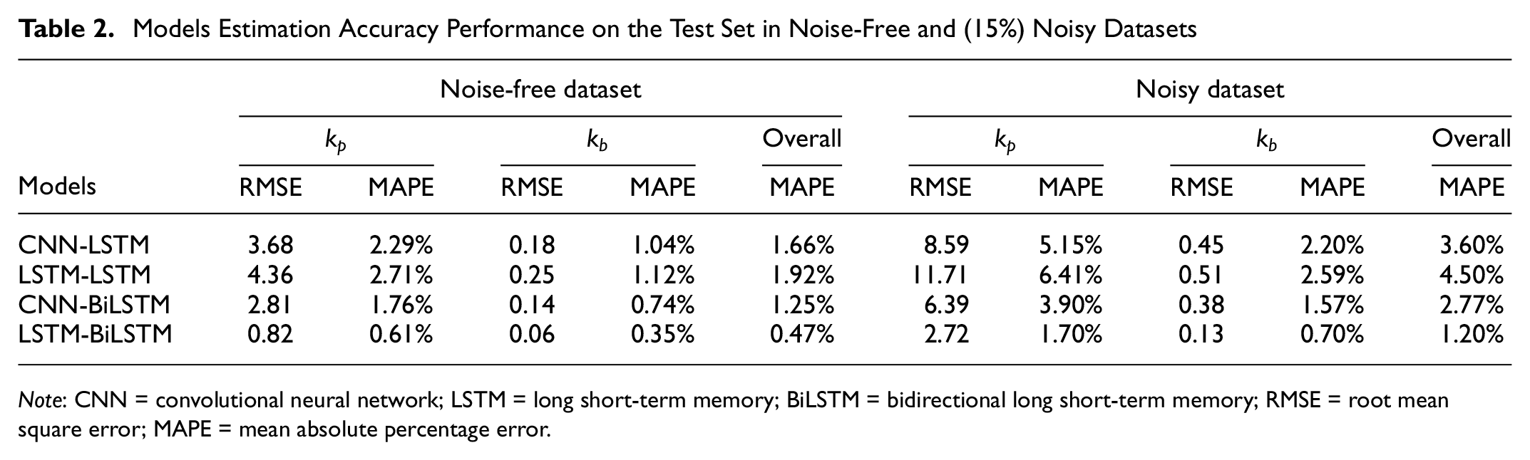
Note: CNN = convolutional neural network; LSTM = long short-term memory; BiLSTM = bidirectional long short-term memory; RMSE = root mean square error; MAPE = mean absolute percentage error.

Table 2 shows the estimation accuracy performance of the four models (CNN-LSTM, LSTM-LSTM, CNN-BiLSTM, and LSTM-BiLSTM) on the test set under two conditions: noise-free and noise-added datasets. The performance metrics include the RMSE and MAPE for two parameters, railpad ( $k_{p}$ ) and ballast ( $k_{b}$ ) stiffness, along with an overall MAPE.

In a noise-free environment, the LSTM-BiLSTM model outperforms the other models, achieving the lowest RMSE for $k_{p}$ at 0.82 (MN/m) and for $k_{b}$ at 0.06 (MN/m). The MAPE values for the LSTM-BiLSTM model are also the lowest, with 0.61% for $k_{p}$ and 0.35% for $k_{b}$ , resulting in an overall MAPE of 0.47%. The CNN-BiLSTM model demonstrated the second-best performance in the noise-free condition. It recorded a RMSE of 2.81 (MN/m) for $k_{p}$ and 0.14 (MN/m) for $k_{b}$ . Its MAPE values are 1.76% for k_p and 0.74% for $k_{b}$ , leading to an overall MAPE of 1.25%. The CNN-LSTM and LSTM-LSTM models rank below their BiLSTM counterparts, with overall MAPEs of 1.66% and 1.92%, respectively.

Under the 15% noise condition, the RMSE and MAPE values for all models increase. However, the LSTM-BiLSTM model remains the best performer, with a RMSE of 2.72 (MN/m) for $k_{p}$ and 0.13 (MN/m)for $k_{b}$ . The MAPE values are 1.70% for $k_{p}$ and 0.70% for $k_{b}$ , resulting in an overall MAPE of 1.20%. The CNN-BiLSTM model continued to show the second-best performance with a RMSE of 6.39 (MN/m) for $k_{p}$ and 0.38 (MN/m) for $k_{b}$ . The MAPE values were 3.90% for $k_{p}$ and 1.57% for $k_{b}$ , leading to an overall MAPE of 2.77%.

The LSTM-BiLSTM and CNN-BiLSTM models consistently outperform the other two models across both datasets. The LSTM-BiLSTM model, in particular, shows low RMSE and MAPE values, highlighting its superior capability in handling both noise-free and noisy data conditions. The LSTM-LSTM and CNN-LSTM models show similar performance in noise-free conditions; however, the LSTM-LSTM model shows poorer performance under noise-added conditions. Overall, all models perform better in predicting ballast stiffness than railpad stiffness.

Figure 5 illustrates the ground truth and predictions for railpad and ballast stiffness in noise-free and noise-added conditions for six railway track segments. The ground truth values of stiffness parameters are represented by the black line, and the estimations in noise-free and noisy conditions are represented with blue and red lines, respectively. Railpad and ballast stiffness are estimated simultaneously in scenarios of constant track stiffness and local stiffness reduction in one and three sleepers.

Figure 5.

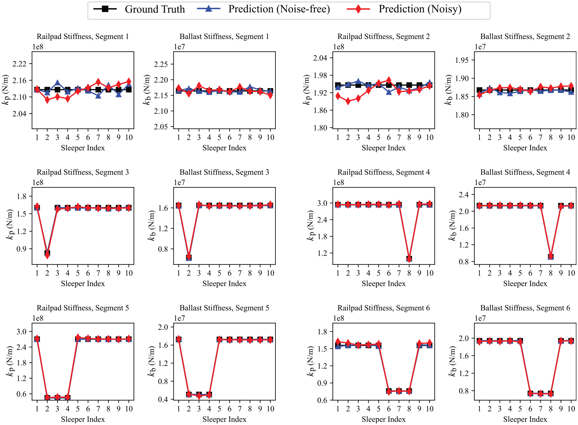
Long short-term memory (LSTM)-bidirectional LSTM model predictions on the noise-added test set, in the scenarios of constant and local changes of stiffness.

Discussion

The illustrative case study demonstrated that the proposed LSTM-BiLSTM model effectively estimates infrastructure stiffness using vehicle-based vibration signals, achieving a MAPE of 1.70% for railpad stiffness and 0.70% for ballast stiffness in the noise-added scenario. The BiLSTM networks outperformed their LSTM counterparts, highlighting the importance of incorporating bidirectional information to enhance infrastructure health monitoring algorithms. The analysis shows that employing BiLSTM in the higher-level health condition estimation phase can reduce the MAPE and RMSE by almost 50%, even in the presence of noise in the input signal. Therefore, this model architecture holds promise for future research and practical applications, given the prevalence of various types of noise in drive-by vibration response measurements.

In the feature extraction phase, the results indicate a nuanced performance pattern among the four model architectures. The best-performing model, LSTM-BiLSTM, employs a LSTM layer in the feature extraction phase, demonstrating the potential of utilizing LSTM layers in this phase. This model outperforms the CNN-BiLSTM model, suggesting that LSTM’s strength in capturing temporal dependencies can be more effective than CNNs when paired with BiLSTM networks. Moreover, the findings underscore the compatibility of BiLSTM networks with both CNN and LSTM feature extractors, as both the CNN-BiLSTM and LSTM-BiLSTM models notably outperform their LSTM counterparts in noise-added scenarios.

The comparative performance of the LSTM-LSTM and CNN-LSTM models introduces complexity in the evaluation of feature extraction methods. The performance of the LSTM-LSTM model slightly falls behind that of the CNN-LSTM model, specifically in noise-added cases. This necessitates further investigation into the utilization of LSTM networks in the feature extraction phase. The literature supports the significance of frequency domain analysis in feature extraction phases, as highlighted in studies such as Shen et al. ( 9 , 34 ) and Lamprea-Pineda et al. ( 39 ). Both approaches, LSTM layers and time–frequency transformations, focus on capturing temporal dependencies along the signal. LSTM networks achieve this through memory cells that learn patterns over time, making them promising candidates for feature extraction ( 40 , 41 ). This similarity points to an area for future research, where further investigations could explore novel feature extraction methods, including LSTM layers, for infrastructure health monitoring models.

The employed CNN and LSTM feature extractors process vibration response data in the time domain. In contrast to previous studies that utilize time–frequency transformations of signals as input for the models ( 26 , 29 ), the proposed method eliminates the need for data preprocessing or hand-crafted feature extraction. Instead, it provides an automatic health condition monitoring framework that learns relevant features directly through the training process. In this approach, we rely on the neural network’s model parameters to extract features from raw vibration signals. However, since drive-by vibration response signals are non-stationary, with components varying in both time and frequency, frequency decompositions may provide valuable insights over the signal ( 42 ). Therefore, future research could investigate novel methodologies that integrate spectral information into deep learning frameworks.

The results indicate that the estimation accuracy of all models decreases in the presence of noise. However, the proposed LSTM-BiLSTM model demonstrates greater robustness to noise compared to the other models, achieving the best performance in the noisy dataset. Despite this, its performance still declines when noise is introduced. Our models solely rely on the neural network parameters learning process to deal with the noise. However, recently, preprocessing techniques have been developed that employ denoising techniques to effectively deal with noisy conditions ( 43 ). Therefore, future research could explore techniques to further enhance the model’s resilience to noise and to develop more robust deep learning frameworks for noisy environments. This is especially important for real-world applications, where noisy data is a common challenge ( 43 ). Moreover, the CNNs employed in the current paper stem from the vanilla CNNs architecture employed by Locke et al. ( 29 ). This can be compared with other machine learning models and recent CNN architectures, such as GoogLeNet and ResNet architectures ( 44 ).

The proposed method effectively identifies and localizes multiple defects within the track segment, with floating locations. It simultaneously estimates railpad and ballast stiffness parameters and localizes stiffness reduction at a sleeper resolution. This enhances infrastructure monitoring tasks by providing detailed information on the type and severity of defects within the railway network. As a result, it can advance maintenance decision-making frameworks by offering comprehensive insights into the health conditions of the systems.

The illustrative case study considers a railway track infrastructure comprising beams and beam nodes. In this context, the rails and the sleepers function as the beams of the structure, while the locations of the sleepers are considered beam nodes that transfer the load to the ballast substructure. The proposed approach involves segmenting the vibration signal into bearing spans corresponding to individual sleepers or beam nodes. This methodology shows potential for application to other infrastructures with a similar configuration of beams and beam nodes, such as bridges.

The dataset used in this study is derived from the vehicle–track interaction finite-element simulation proposed by Shen et al. ( 9 ). While this case study demonstrates the proposed framework, simulated vehicle–track interaction signals may not fully capture all environmental and operational factors influencing drive-by measurements. For instance, the dataset in the current work assumes a constant measurement speed as the operational condition, whereas real-world drive-by measurements may involve speed variations. In addition, the simulated dataset represents a single type of railway track structure, whereas real-world railway networks may exhibit structural variations. Therefore, this study opens new research directions for evaluating the performance of the proposed LSTM-BiLSTM network using field measurements of drive-by vibration responses.

Conclusions and Future Work

In this paper, we proposed a novel method for estimating and localizing multiple physical parameters of infrastructures using drive-by vibration responses, achieved through the development of a LSTM-BiLSTM network. Our approach highlights the importance of utilizing both forward and backward temporal information via BiLSTM networks to improve algorithms for monitoring the health conditions of infrastructures. The findings demonstrate that incorporating BiLSTM networks in the higher-level health condition estimation phase significantly reduces both the MAPE and RMSE, even in the presence of noise. Moreover, the methodology highlights the potential of LSTM networks for extracting features from drive-by vibration signals. By accurately identifying the positions of vibration signals, our proposed framing approach improves the resolution of infrastructure monitoring to the beam level. Therefore, the LSTM-BiLSTM model effectively estimates physical parameters at various components within the infrastructure beam levels, offering valuable insights into the health conditions of these systems and improving maintenance decision-making frameworks. In the case study analyzed, the results show that the method is effective in estimating the stiffness parameters of railpads and ballast, as well as in identifying track stiffness reductions at individual sleepers. The proposed BiLSTM networks significantly decrease the MAPE and RMSE by nearly 50%, achieving a MAPE of 1.7% for railpad stiffness and 0.7% for ballast stiffness, even in noisy environments.

Future research will focus on three main research directions. Firstly, the proposed hybrid model architecture requires further benchmarking against state-of-the-art methodologies. This includes considering advanced CNN and LSTM networks alongside other machine learning methods. Secondly, future research should validate the performance of the proposed models based on field measurements and under real-world conditions. This further requires developing deep learning models that are robust to real-world noisy environments. Thirdly, the proposed framing approach requires high-accuracy signal localization, which can be challenging under certain operational conditions. In this regard, leveraging domain knowledge concerning the number of beam nodes in certain infrastructure lengths holds promise for addressing the signal localization challenge.

Footnotes

Acknowledgements

The first author would like to extend their gratitude to Chen Shen for providing the simulator used in this article. The first author would like to extend their gratitude to Yuanchen Zeng and Hesam Araghi for their valuable comments during the preparation of this article.

Author Contributions

The authors confirm contribution to the paper as follows: study conception and design: R.R. Samani, A. Núñez, B. De Schutter; data collection: R.R. Samani, A. Núñez; analysis and interpretation of results: R.R. Samani, A. Núñez; draft manuscript preparation: R.R. Samani, A. Núñez, B. De Schutter. All authors reviewed the results and approved the final version of the manuscript.

Declaration of Conflicting Interests

The author(s) declared no potential conflicts of interest with respect to the research, authorship, and/or publication of this article.

Funding

The author(s) disclosed receipt of the following financial support for the research, authorship, and/or publication of this article: This research was partly supported by ProRail and Europe's Rail Flagship Project IAM4RAIL—Holistic and Integrated Asset Management for Europe's Rail System (grant agreement 101101966).

ORCID iDs

Reza Riahi Samani

Alfredo Nunez Vicencio

Bart De Schutter

Funded by the European Union. Views and opinion expressed are however those of the authors(s) only and do not necessarily reflect those of the European Union. Neither the European Union nor the granting authority can be held responsible for them. This project has received funding from the European Union's Horizon Europe research and innovation programme under Grant Agreement No 101101966.

References

Ghofrani

Mohammadi

Pathak

Aref

Bayesian Survival Approach to Analyzing the Risk of Recurrent Rail Defects. Transportation Research Record: Journal of the Transportation Research Board, 2019. 2673: 281–293.

Mohammadi

Ghofrani

Pathak

Aref

Exploring the Relationship between Foot-by-Foot Track Geometry and Rail Defects: A Data-Driven Approach. Presented at 98th Annual Meeting of Transportation Research Board, Washington, D.C., 2019.

Radzieński

Krawczuk

Palacz

Improvement of Damage Detection Methods Based on Experimental Modal Parameters. Mechanical Systems and Signal Processing, Vol. 25, 2011, pp. 2169–2190.

Neuhold

Landgraf

Marschnig

Veit

Measurement Data-Driven Life-Cycle Management of Railway Track. Transportation Research Record: Journal of the Transportation Research Board, 2020. 2674: 685–696.

Movaghar

Mohammadzadeh

Intelligent Index for Railway Track Quality Evaluation Based on Bayesian Approaches. Structure and Infrastructure Engineering, Vol. 16, 2019, pp. 968–986.

Movaghar

Mohammadzadeh

Bayesian Monte Carlo Approach for Developing Stochastic Railway Track Degradation Model Using Expert-Based Priors. Structure and Infrastructure Engineering, Vol. 18, 2020, pp. 145–166.

Nielsen

J. C.

Berggren

E. G.

Hammar

Jansson

Bolmsvik

Degradation of Railway Track Geometry – Correlation Between Track Stiffness Gradient and Differential Settlement. Proceedings of the Institution of Mechanical Engineers, Part F: Journal of Rail and Rapid Transit, Vol. 234, No. 1, 2020, pp. 108–119.

Hoelzl

Dertimanis

Ancu

Kollros

Chatzi

Vold–Kalman Filter Order Tracking of Axle Box Accelerations for Track Stiffness Assessment. Mechanical Systems and Signal Processing, Vol. 204, 2023, p. 110817.

Shen

Zhang

Dollevoet

Zoeteman

, Evaluating Railway Track Stiffness Using Axle Box Accelerations: A Digital Twin Approach. Mechanical Systems and Signal Processing, Vol. 204, 2023, p. 110730.

10.

Fernández-Bobadilla

H. A.

Martin

, Modern Tendencies in Vehicle-Based Condition Monitoring of the Railway Track. IEEE Transactions on Instrumentation and Measurement, Vol. 72, 2023, pp. 1–44.

11.

Alvandi

Cremona

, Assessment of Vibration-Based Damage Identification Techniques. Journal of Sound and Vibration, Vol. 292, 2006, pp. 179–202.

12.

Quirke

Cantero

OBrien

E. J.

Bowe

, Drive-by Detection of Railway Track Stiffness Variation Using in-Service Vehicles. Proceedings of the Institution of Mechanical Engineers, Part F: Journal of Rail and Rapid Transit, Vol. 231, 2017, pp. 498–514.

13.

Zhu

X. Q.

Law

S. S.

Huang

, Identification of Railway Ballasted Track Systems from Dynamic Responses of In-Service Trains. Journal of Aerospace Engineering, Vol. 31, 2018, p. 04018060.

14.

Avci

Abdeljaber

Kiranyaz

Hussein

Gabbouj

Inman

D. J.

, A Review of Vibration-Based Damage Detection in Civil Structures: From Traditional Methods to Machine Learning and Deep Learning Applications. Mechanical Systems and Signal Processing, Vol. 147, 2021, p. 107077.

15.

Phusakulkajorn

Núñez

Wang

Jamshidi

Zoeteman

Ripke

Dollevoet

De Schutter

Artificial Intelligence in Railway Infrastructure: Current Research, Challenges, and Future Opportunities. Intelligent Transportation Infrastructure, Vol. 2, 2023, p. liad016.

16.

Zaman

Liu

Zhang

Video Analytics for Railroad Safety Research: An Artificial Intelligence Approach. Transportation Research Record, Vol. 2672, 2018, pp. 269–277.

17.

Sony

Towards Multiclass Damage Detection and Localization Using Limited Vibration Measurements. Ph.D. thesis, University of Western Ontario, 2021.

18.

Hung

D. V.

Hung

H. M.

Anh

P. H.

Thang

N. T.

Structural Damage Detection Using Hybrid Deep Learning Algorithm. Journal of Science and Technology in Civil Engineering (JSTCE) - HUCE, Vol. 14, 2020-04-17, pp. 53–64.

19.

Rafe

Singleton

P. A.

Imputing Time Series Pedestrian Volume Data With Consideration of Epidemiological-Environmental Variables. Transportation Research Record: Journal of the Transportation Research Board, 2024. 2678: 281–298.

20.

Rafe

Singleton

P. A.

Exploring Factors Affecting Pedestrian Crash Severity Using TabNet: A Deep Learning Approach. Data Science for Transportation, Vol. 6, 2024, p. 13.

21.

Rafe

Singleton

P. A.

Exploring the Complexity of Pedestrian Dynamics: Impact of Societal Behaviors and Personal Attributes in Urban Environments. Transportation Research Record: Journal of the Transportation Research Board, 2024. 2679: 136–160.

22.

Riahi Samani

Riahisamani

Mishra

Golias

M. M.

Jung-Hwi Lee

Evaluating Relocation Behavior of Establishments: Evidence for the Short-Term Effects of COVID-19. Environment and Planning B: Urban Analytics and City Science, Vol. 51, No. 9, 2024, pp. 2012–2030.

23.

Yan

T.-H.

Costa

M. D. A.

Corman

Developing and Extending Status Prediction Models for Railway Tracks Based on On-Board Monitoring Data. Transportation Research Record: Journal of the Transportation Research Board, 2023. 2677: 708–719.

24.

Chellaswamy

Geetha

T. S.

Surya Bhupal Rao

Vanathi

Optimized Railway Track Condition Monitoring and Derailment Prevention System Supported by Cloud Technology. Transportation Research Record: Journal of the Transportation Research Board, Vol. 2675, 2021, pp. 346–361.

25.

Hajializadeh

Deep Learning-Based Indirect Bridge Damage Identification System. Structural Health Monitoring, Vol. 22, 2023, pp. 897–912.

26.

Pathirage

C. S. N.

Hao

Liu

Structural Damage Identification Based on Autoencoder Neural Networks and Deep Learning. Engineering Structures, Vol. 172, 2018, pp. 13–28.

27.

Huang

Yin

Kaewunruen

Quantification of Dynamic Track Stiffness Using Machine Learning. IEEE Access, Vol. 10, 2022, pp. 78747–78753.

28.

Le-Xuan

Bui-Tien

Tran-Ngoc

A Novel Approach Model Design for Signal Data Using 1DCNN Combing with LSTM and ResNet for Damaged Detection Problem. Structures, Vol. 59, 2024, p. 105784.

29.

Locke

Sybrandt

Redmond

Safro

Atamturktur

Using Drive-by Health Monitoring to Detect Bridge Damage Considering Environmental and Operational Effects. Journal of Sound and Vibration, Vol. 468, 2020, p. 115088.

30.

Jie

Fang

Weiping

Xiaoxiong

Track Vibration Sequence Anomaly Detection Algorithm Based on LSTM. Advances in Structural Engineering, Vol. 26, 2023, pp. 1682–1695.

31.

Sharma

Sen

Real-Time Structural Damage Assessment Using LSTM Networks: Regression and Classification Approaches. Neural Computing and Applications, Vol. 35, 2023, pp. 557–572.

32.

Hochreiter

Schmidhuber

Long Short-Term Memory. Neural Computation, Vol. 9, 1997, pp. 1735–1780.

33.

Samani

R. R.

Data underlying the publication: A Bidirectional Long Short Term Memory Approach for Infrastructure Health Monitoring Using On-board Vibration Response. Version 1. 4TU.ResearchData. dataset., 2025. https://doi.org/10.4121/64600497-7ba5-4831-9c94-1b643f600987.v1.

34.

Shen

Dollevoet

Fast and Robust Identification of Railway Track Stiffness from Simple Field Measurement. Mechanical Systems and Signal Processing, Vol. 152, p. 107431.

35.

Kaewunruen

Remennikov

A. M.

Field Trials for Dynamic Characteristics of Railway Track and Its Components Using Impact Excitation Technique. NDT & E International, Vol. 40, pp. 510–519.

36.

Shi

Zhou

Zhang

Guo

A Critical Review on the Vertical Stiffness Irregularity of Railway Ballasted Track. Construction and Building Materials, Vol. 400, 2023, p. 132715.

37.

González

Feng

Casero

Effective Separation of Vehicle, Road and Bridge Information from Drive-by Acceleration Data via the Power Spectral Density Resulting from Crossings at Various Speeds. Developments in the Built Environment, Vol. 14, 2023, p. 100162.

38.

Malekjafarian

Golpayegani

Moloney

Clarke

A Machine Learning Approach to Bridge-Damage Detection Using Responses Measured on a Passing Vehicle. Sensors, Vol. 19, 2019, p. 4035.

39.

Lamprea-Pineda

A. C.

Connolly

D. P.

Castanheira-Pinto

Alves-Costa

Hussein

M. F.

Woodward

P. K.

On Railway Track Receptance. Soil Dynamics and Earthquake Engineering, Vol. 177, 2024, p. 108331.

40.

Malhotra

Ramakrishnan

Anand

Vig

Agarwal

Shroff

LSTM-based Encoder-Decoder for Multi-sensor Anomaly Detection. ICML 2016 Anomaly Detection Workshop, New York, NY, 2016. https://doi.org/10.48550/arXiv.1607.00148.

41.

Hou

Yang

Wang

Yan

LSTM-Based Auto-Encoder Model for ECG Arrhythmias Classification. IEEE Transactions on Instrumentation and Measurement, Vol. 69, 2020, pp. 1232–1240.

42.

Nossier

S. A.

Wall

Moniri

Glackin

Cannings

A Comparative Study of Time and Frequency Domain Approaches to Deep Learning Based Speech Enhancement. In 2020 International Joint Conference on Neural Networks (IJCNN), Glasgow, UK, 2020, pp. 1–8.

43.

Michau

Frusque

Fink

Fully Learnable Deep Wavelet Transform for Unsupervised Monitoring of High-Frequency Time Series. Proceedings of the National Academy of Sciences, Vol. 119, 2022, p. e2106598119.

44.

Szegedy

Ioffe

Vanhoucke

Alemi

Inception-v4, Inception-ResNet and the Impact of Residual Connections on Learning. Proceedings of the AAAI Conference on Artificial Intelligence, Vol. 31, No. 1, 2017.

Bidirectional Long Short-Term Memory Approach for Infrastructure Health Monitoring Using On-Board Vibration Response

Abstract

Keywords

Deep Learning in Structure Health Monitoring using Vibration Response

Contributions of this Paper

Preliminaries

LSTM Cell

1D Convolutional Neural Networks

Methodology

Problem Statement

Lower-Level Bearing Span Feature Extractor

1DCNN

LSTM

Upper-Level BiLSTM Networks

Illustrative Case Study of Railway Track Monitoring

Data

Results

Discussion

Conclusions and Future Work

Footnotes

Acknowledgements

Author Contributions

Declaration of Conflicting Interests

Funding

ORCID iDs

References