Sage Journals: Discover world-class research

Abstract

This study focuses on developing a synthetic population for Nova Scotia to update the base-year synthesis for an agent-based integrated transport and land use model. It proposes a novel population synthesizer, developed in Python programming language. Utilizing the 2016 hierarchical public use microdata file (PUMF) and census data, the iterative proportional updating algorithm was employed to generate the synthetic data at the county level, followed by conditional Monte Carlo simulation for micro spatial unit assignment to the dissemination area. A feedforward neural network (FNN) model is used to tackle missing value issues in the PUMF data and added the capacity to synthesize base-year mobility tool ownership. The addition of missing values enhanced the distribution accuracy of the PUMF against census totals. The synthesis process generated individuals with an error percentage of 0.07% compared to the actual population. Most household-level and individual-level attributes had an error between −0.5% and +0.5%, while a few attributes showed errors slightly outside this range. The synthetic data shows a close joint distribution to the PUMF. Household vehicle ownership, driver’s license holders, and transit pass ownership were added to the synthetic data using a FNN model. The FNN model achieved an overall accuracy of 52% for vehicle ownership, with 87% predictions within ±1 vehicle per household. Although the model demonstrates 90% overall accuracy for driver’s license ownership, and 92% for transit pass owners, it showed lower precision and recall for non-driver’s license holders and transit pass holders because of their low dataset representation.

Keywords

machine learning data and data science neural networks planning and analysis transportation demand forecasting models/modeling

Transportation models have evolved from aggregated trip-based to disaggregated agent-based models (ABMs) over the past few decades. The agent-based microsimulation transport models simulate the complex decision-making and the dynamic interaction of multiple elements while considering the diverse behaviors of individuals and households, and they result in greater accuracy than the traditional four-stage models ( 1 ). However, the successful implementation of these models depends on the availability of detailed household and person attribute data, which is often incomplete or unavailable in a disaggregate form for the entire region. Collecting such data for the whole population is expensive with respect to time and resources. Disaggregated data may be available for a small sample population through a travel activity survey or census data. In Canada, although such data is collected for the entire population through census data, it is not available for public use because of privacy policy. Rather, such data is published without revealing any personal identification of individuals for a sample population (1%–2.5% depending on the type of data), referred to as a public use microdata file (PUMF). An efficient solution to producing socio-demographic information for an entire region is to develop synthetic populations representing the actual distribution of individual- and household-level attributes of the target study area. This process is often termed “population synthesis” in transportation demand analysis, and synthetic datasets can serve as inputs for ABMs. Population synthesis utilizes two types of data: microsample data for a sample population in the target area and the aggregated marginal totals at the target level of spatial resolution. The key challenge is integrating these two data sources to accurately represent individual- and household-level attributes. There are several methods used to combine these two types of data to produce a synthetic population, such as fitting methods, probabilistic models, simulation-based (SB) models, and machine learning techniques ( 2 ).

One key challenge in adopting any survey data or microsample is the presence of missing attributes in some household and individual entries. Removing such entries from the sample data may result in an inadequate sample size or alter the distribution of certain attributes, potentially skewing the data. Addressing these missing attributes is crucial as they can lead to biased results. Another challenge in selecting a microsample is that it may not contain all the target attributes needed as input for ABMs. For instance, census PUMF data do not include mobility tool-related attributes, such as vehicle ownership, whereas some travel activity surveys do. However, the census PUMF generally provides a better representation of the real world compared to survey data. Therefore, it is essential to use the PUMF while also integrating other data sources to include the necessary attributes in the synthetic data.

The primary objective of this study is to develop a synthetic population for Nova Scotia, addressing the challenges outlined earlier. The synthetic data will serve as an input for two operational models: an agent-based integrated transportation land use and energy model (iTLE) for the Halifax Regional Municipality (HRM) and a provincial-level travel demand model for Nova Scotia. The iTLE simulates individuals' long-term and short-term decisions, leading to traffic simulation and emission modeling. A prototype iTLE has been developed for the HRM and is currently operational ( 3 ). To achieve the objective, the study builds on four major steps. (1) Developing a novel population synthesizer using Python programming language. (2) Addressing the missing attributes in the PUMF data samples to ensure a complete dataset. (3) Developing a synthetic population for Nova Scotia that includes key individual and household characteristics. Utilizing the PUMF data and census aggregate targets, the study employed the iterative proportional updating (IPU) algorithm for this process. (4) Adding the base-year mobility tool ownership to the synthetic population, which is not available in the PUMF database to incorporate within the IPU process. Utilizing the Nova Scotia Travel Activity (NovaTRAC) survey data collected across Nova Scotia, the study used deep learning models to add household vehicle ownership, individual driver’s license, and transit pass ownership attributes to the synthetic population.

Literature Review

Population Synthesis Methods

Developing synthetic data for the target population has become pivotal in several sectors, including public health, engineering, and transport modeling. Synthetic data is crucial in the modern world as it allows the development of realistic datasets while maintaining privacy and confidentiality, facilitating the development and testing of advanced algorithms without risking sensitive information. In the transportation sector, synthetic agents with their individual- and household-level attributes have been the primary input for agent-based travel demand models. One key consideration in developing synthetic populations is to ensure that the joint distribution of key household and individual attributes in the synthetic population aligns with the known aggregate distributions from census data.

The population synthesis process involves two main stages: the fitting stage and the generation stage. During the fitting stage, a disaggregated microsample is weighted using an iterative reweighting procedure to align with a set of target marginal distributions. In the generation stage, the actual population is created based on these weights ( 4 ). One of the traditional methods for generating synthetic populations is iterative proportional fitting (IPF). The IPF method was introduced by Deming and Stephan in 1940 ( 5 ), and Beckman et al. ( 6 ) first adopted it for transport research to develop a synthetic population for the TRANSIMS system. IPF involves iterative steps where each row and column are proportionally adjusted to match the marginal row and column totals. These steps are repeated until both rows and columns converge or the sum of the rows and columns is relatively close to their marginal totals. The fundamental assumption in fitting methods is that the sample accurately reflects the actual correlation structure among the attributes.

Although IPF is an efficient fitting method, it has certain practical limitations. One of the primary concerns in IPF is the "zero-cell problem," which occurs when certain household types are missing in the seed data, making it impossible to calculate the odds ratio ( 5 ). Also, IPF cannot differentiate between structural and sampling zero. Various methods have been proposed in the literature to avoid sampling zero issues, notably by Guo and Bhat ( 7 ) and Auld et al. ( 8 ). Secondly, the joint distribution's complexity increases significantly with more control tables and categories, leading to higher demands on computational resources such as memory. Pritchard and Miller ( 9 ) employed sparse matrix manipulation techniques to address this problem. The second stage of IPF-based methods includes producing a synthetic population using the adjusted contingency table. This process involves duplicating the sample based on the weights of each cell. To integrate fractions into the synthetic population, inverse transform sampling is utilized in a Monte Carlo simulation ( 6 ). Prédhumeau and Manley ( 10 ) developed an open-source synthetic population for Canada using IPF combined with quasi-random integer sampling (QISI) to ensure accurate integer-based outputs. The study highlights that QISI offers a balance between efficiency and accuracy, avoiding mismatches from traditional methods. However, the authors note that QISI becomes computationally intensive for attributes with many categories.

One of the original IPF algorithm's major limitations is that it cannot simultaneously match household- and individual-level attributes. Arentze et al. ( 11 ) used relation matrices to convert the individual to household distributions, controlling person-level marginal distributions. Guo and Bhat ( 7 ) proposed an algorithm for generating synthetic populations that improve person-level distribution fits. Zhu and Ferreira ( 12 ) introduced hierarchical iterative proportional fitting (HIPF), a multistage IPF procedure. In line with these modifications, Ye et al. ( 13 ) introduced the IPU technique to control household- and individual-level attributes simultaneously. Ye et al. ( 14 ) updated this algorithm to a bi-level optimization to include more than one social organization. Like IPU, the combinatorial optimization (CO) method controls both household- and individual-level attributes ( 15 ). This approach utilizes optimization techniques such as simulated annealing (SA) to minimize discrepancies between the synthetic population and marginal totals ( 16 ). Hafezi and Habib ( 17 ) advanced the use of fitness-based synthesis (FBS), including multilevel controls, by selecting variables with the highest fitness.

To better address the complexity and richness of real-world populations, SB approaches have emerged as strong alternatives to fitting techniques. These methods allow for flexible modeling of high-dimensional joint distributions and offer improved performance when data is sparse or partially missing. Farooq et al. ( 18 ) proposed a Markov chain Monte Carlo (MCMC) simulation approach for population synthesis. The study shows that the MCMC-based method outperformed the IPF approach with respect to the standard root mean square error (SRMSE), especially under sparse data conditions. However, they also noted that the MCMC approach requires tuning and is computationally more intensive, especially when dealing with large populations. Saadi et al. ( 19 ) employed hidden Markov models (HMMs) for synthetic population generation. Their study found that HMMs provided a better fit than IPF, particularly when sample sizes were small. They also reported that HMMs naturally capture sequence-based dependencies, which enhances their performance in modeling household structures. The study also acknowledged that estimating transition probabilities becomes challenging with the increasing number of attributes.

Rahman and Fatmi ( 20 ) proposed a Bayesian network with a generalized raking (BN-GR) approach for population synthesis that accommodates heterogeneity across household and individual attributes. The study highlights that this approach is capable of handling missing or incomplete data and capturing interdependencies between attributes. Zhang et al. ( 21 ) used a hierarchical Bayesian network for generating synthetic populations, introducing latent variables to represent hidden groupings among household structures. Their model learns both the network structure and parameters from data, and they report improved fit and flexibility over traditional flat BN models. Ilahi and Axhausen ( 22 ) integrated a Bayesian network with a multilevel IPF method for Greater Jakarta. Borysov et al. ( 23 ) introduced a deep generative modeling approach using variational autoencoders (VAEs). The study demonstrated that VAEs outperform conventional methods in capturing complex and high-dimensional relationships among synthetic agents. The authors noted that their approach avoids simple replication of observed agents and can handle sparse regions of the attribute space effectively. However, they mentioned that VAEs require a significant volume of data for training.

Fabrice Yaméogo et al. ( 2 ) offered a comprehensive review and comparison of several synthetic population generation techniques, including synthetic reconstruction (SR), CO, and SB approaches. The study developed a decision tree to help researchers identify the most appropriate synthesis method based on data availability and use-case complexity. They concluded that SB methods, particularly statistical learning techniques such as BNs and VAEs, are highly suited for applications involving incomplete data, high-dimensional variables, or complex attribute interdependencies. Nonetheless, they highlighted that these methods are generally more data-demanding and require careful model specification ( 2 ). One major challenge in statistical approaches is to distribute the synthetic population developed for the region into micro spatial units, such as traffic analysis zones. Several researchers have used the generalized raking (GR) algorithm to fit the synthetic data to microspatial units (20,22).

Mobility Tool Ownership Modeling

Base-year mobility tool ownership is a key attribute in a synthesized population for agent-based transport models. Several studies have used discrete choice models such as multinomial logit models, nested logit models, cross-nested logit models, and multivariate probit models to predict mobility tool ownership ( 24 ). In recent years, several transportation studies have adopted machine learning algorithms to predict transportation-related characteristics of individuals and households. Artificial neural networks (ANNs) are non-linear statistical models that can be utilized for regression and classification tasks in machine learning applications. ANNs differ from discrete choice methods by using pattern association and error correction to represent problems, whereas discrete choice methods rely on the random utility maximization rule ( 25 ). A neural network typically consists of three layers: input nodes receiving signals, output nodes delivering outputs, and potentially numerous intermediate layers with intermediate nodes ( 26 ). Neural networks come in various types and architectures. Common forms include perceptrons, backpropagation networks, Kohonen self-organizing maps, continuous adaptive time networks, time-delay neural networks, and recurrent neural networks, among others ( 26 ). Backpropagation networks are neural networks featuring hidden layers. They initially assign random weights to their synapses and are trained by being exposed to input values paired with the correct output values. Throughout training, the network adjusts these weights to enhance the accuracy of its responses ( 27 ).

Several studies compared the accuracy of machine learning models and discrete choice models in predicting the mobility-related attributes of agents. Basu and Ferreira ( 28 ) compared several machine learning algorithms with the multinomial logit model and ordinal logit model to predict household vehicle ownership. The study results show that the ordinal logit classification approach with neural network binary classifiers and an ANN algorithm gives better accuracy than multinomial logit models. Mohammadian and Miller ( 27 ) compared the performance of nested logit models and ANNs to predict automobile choices. The ANN model classified 70.38% correctly, and the Nested Logit Model (NLM) predicted only 49.2% correctly ( 27 ). Rajalakshmi ( 29 ) utilized an ANN model for mode choice modeling of work-based trips in India. In their study, Dixon et al. ( 30 ) found that neural networks can predict car ownership with 29% less error than linear regression models. In their study, Pueschel et al. ( 24 ) compared discrete choice models and machine learning approaches for simultaneously predicting multiple mobility tools, car ownership, driver’s license, and transit pass, within an agent-based travel demand modeling framework. Their results showed that shallow neural networks outperformed uncalibrated discrete choice models with respect to predictive accuracy, while also offering easier formulation and application to synthetic populations.

Although several studies show deep learning algorithms, such as neural networks, yield better accuracy than econometric and regression models, they have a very low interpretability of independent variables. This could pose a complexity to run future policy-related scenarios as the independent variable effects are hard to interpret. Another complexity in using machine learning models for prediction models is their complexity of post-training calibration compared to discrete choice models. The post-training calibration of machine learning models can be improved using probability scaling methods such as Platt scaling or isotonic regression ( 31 ), although they remain less intuitive than coefficient adjustments in logit models.

This study addressed one of the major concerns in microsamples, which is missing and incomplete information on some attributes. The study also utilizes an ANN approach when incorporating additional attributes such as household vehicle ownership, driver’s license owners, and transit pass owners into the synthetic population, which were not present in the microsample used for the synthesis process. This study utilized a fitting algorithm (IPU) and a neural network model (feedforward neural network [FNN]) with two different microsamples (the PUMF and NovaTRAC survey data) to develop a synthetic population as the base-year input for an agent-based travel demand model.

Data Source

Nova Scotia is one of the Atlantic provinces in Canada. According to census data, the total population was 920,070 in 2016 and 969,383 in 2021. Nova Scotia includes 18 counties, of which Halifax County makes up around 40% of the population. There are also six municipalities in the province. The population synthesis was developed at the micro spatial level of dissemination areas (DAs), and Nova Scotia consists of 1593 DAs. Figure 1 shows the study area and the counties in Nova Scotia.

Figure 1.

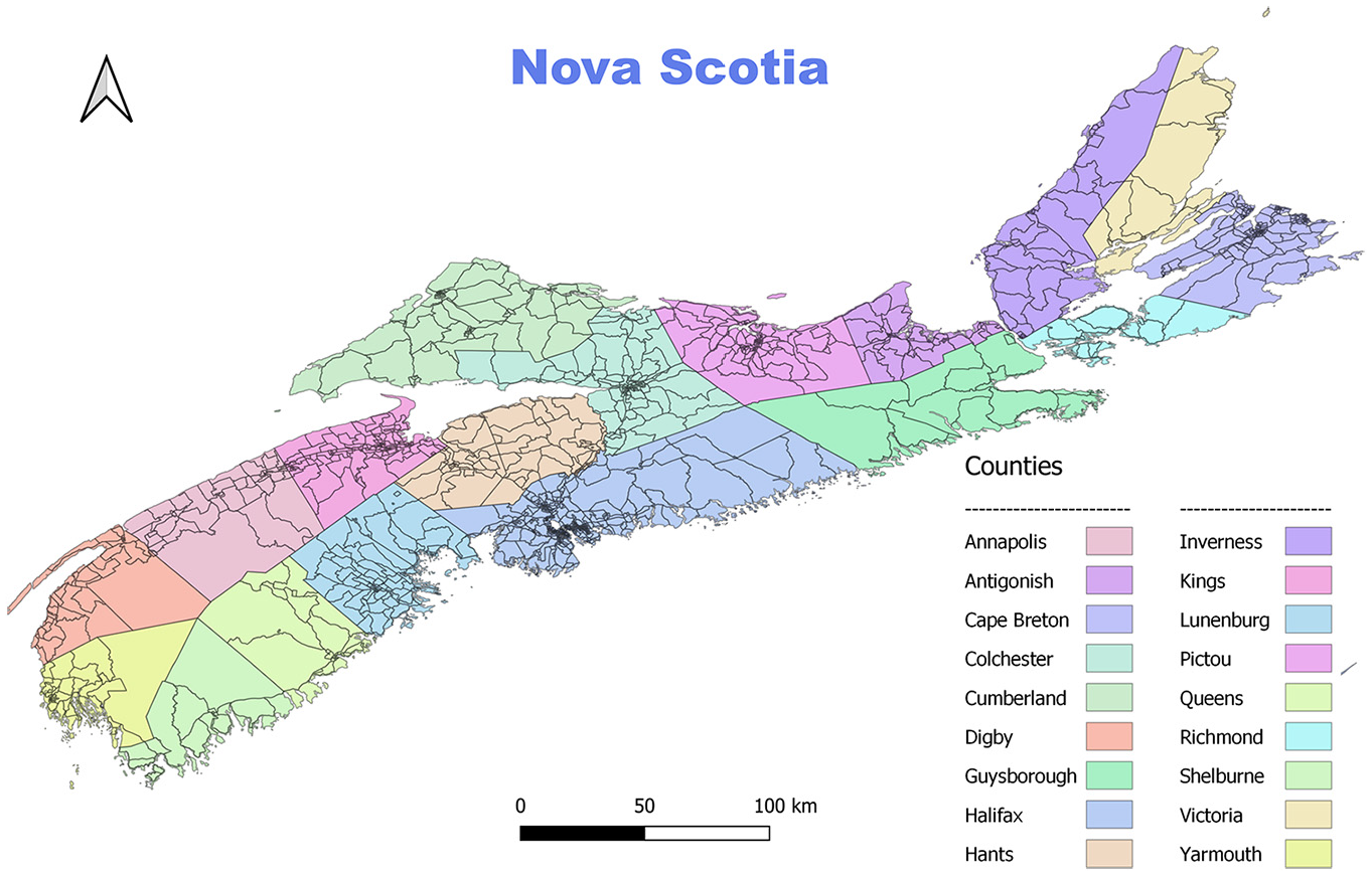
Study area—Nova Scotia.

Population synthesis is performed utilizing the 2016 hierarchical PUMF and the 2016 census data from Statistics Canada. The PUMF data is unavailable at a disaggregated level, such as DA or county levels. Instead, the microdata is available at an aggregated spatial level of Nova Scotia and is utilized for this study. The hierarchical PUMF data file includes detailed information on 4020 households and 9077 individuals within those households. The PUMF includes various demographic and socioeconomic data about households, families, and individuals. However, specific details such as exact locations, income information, and other particulars are omitted for privacy reasons. The aggregated marginal totals from the 2016 Canadian Census for the study area include 920,070 individuals and 401,890 households. The control variables were selected to align with the input requirements of the iTLE. At the household level, these include household income, household size, tenure type, and dwelling type, and at the individual level, age, sex, employment status, and marital status, following the specification outlined by Fatmi ( 32 ). A detailed breakdown of the distribution of each attribute in the PUMF data and census target data is shown in Table 1.

Table 1.

Individual- and Household-Level Attributes

		PUMF		Census DA level
Attribute	Category	Samples	%	Target	%
Individual level
Gender	Male	4372	48.16	446,695	48.41
	Female	4705	51.84	476,050	51.59
Age group	0–14	1259	13.87	133,789	14.50
	15–19	466	5.13	51,092	5.54
	20–24	469	5.17	56,006	6.07
	25–29	543	5.99	53,682	5.82
	30–34	502	5.53	51,567	5.59
	35–39	520	5.73	52,162	5.65
	40–44	537	5.91	56,946	6.17
	45–49	635	7.00	61,770	6.69
	50–54	764	8.42	75,698	8.20
	55–64	1554	17.12	146,537	15.88
	65–74	1155	12.72	108,648	11.77
	75 and above	672	7.41	74,848	8.11
Marital status	Never married	3236	35.65	343,287	37.20
	Married	3787	41.72	369,532	9.24
	Living in common law	838	9.23	85,222	13.51
	Separated/widowed/divorced	1217	13.41	124,704	13.51
Employment	Employed	4338	47.79	434,001	47.03
	Unemployed	436	4.81	48,102	5.21
	Not in the labor force	3044	33.54	304,750	33.03
	Minors	1259	13.87	135,892	14.73
Household level
Income	C$ 0–20,000	491	12.22	46,694	11.62
	C$20,000–49,000	1201	29.87	118,011	29.36
	C$50,000–79,000	904	22.49	91,715	22.82
	C$80,000–99,000	435	10.81	44,497	11.07
	C$100,000 and above	990	24.62	100,974	25.12
Household size	1 person	1239	30.83	118,767	29.55
	2 persons	1628	40.50	156,771	39.01
	3 persons	601	14.95	60,286	15.00
	4 persons	419	10.42	44,859	11.16
	5 persons and above	133	3.30	21,207	5.28
Tenure type	Owner	2748	68.36	277,654	69.09
	Rent	1272	31.64	124,236	30.91
Dwelling type	Single detached	2653	66.00	263,500	65.57
	Apartment	920	22.87	92,040	22.90
	Others	447	11.13	46,350	11.53

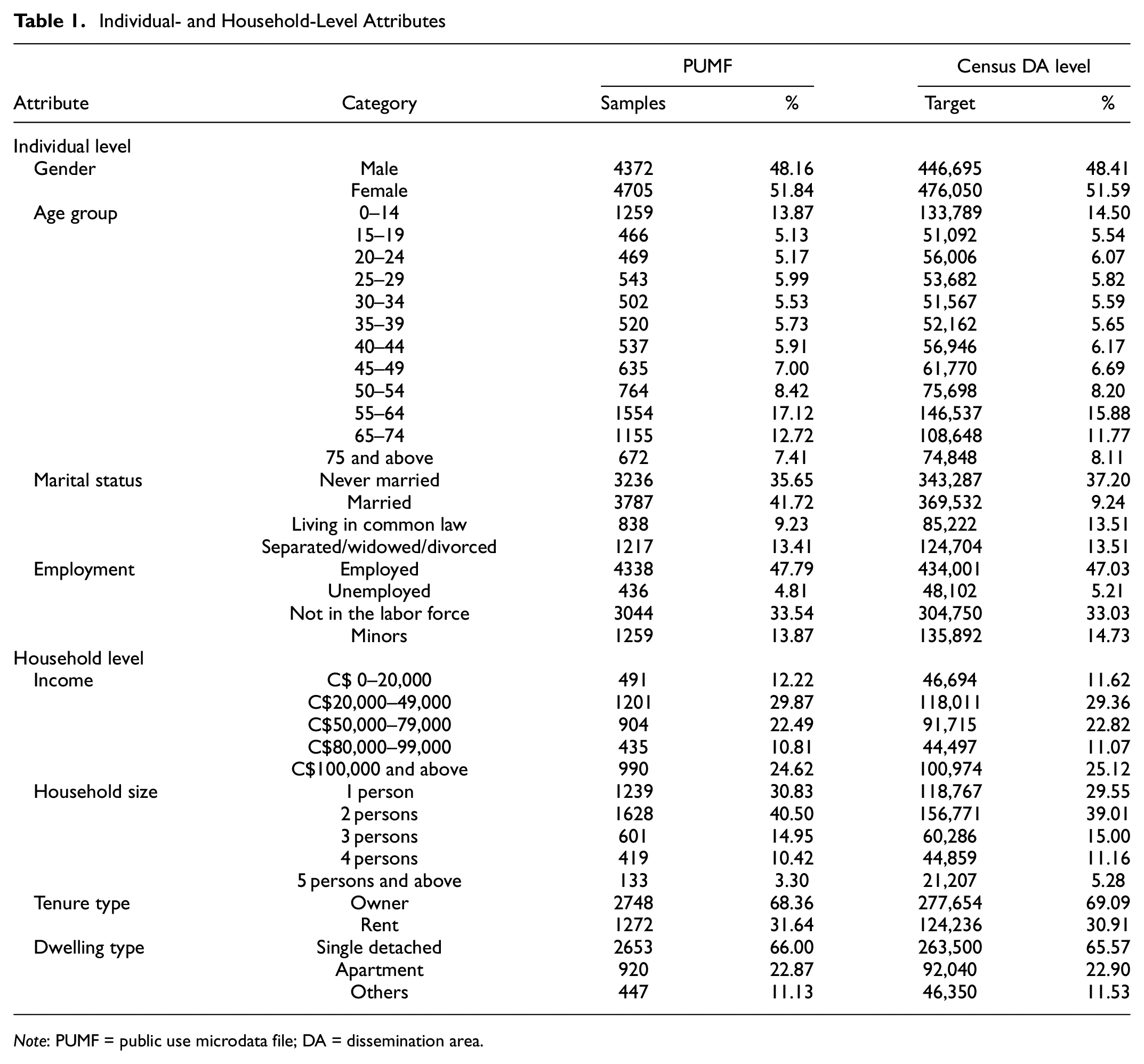
Note: PUMF = public use microdata file; DA = dissemination area.

Some key household and individual attributes relevant to travel demand modeling, such as household vehicle ownership, driver’s license ownership, and transit pass ownership, are not included in the PUMF data. Consequently, these attributes could not be incorporated as control variables during the synthesis process. The NovaTRAC survey conducted during the 2022–2023 period were utilized to estimate and expand the synthetic data to include these variables. The NovaTRAC data includes detailed socio-demographic information of 4868 households and 6662 household members within those households. The survey collected household- and individual-level socio-demographic characteristics and their 24-h travel activity log. The survey includes the three target attributes of this study, household vehicle ownership, individual's driver’s license, and transit pass ownership details.

Methodology

The primary input for agent-based travel demand models is a base-year synthetic population that includes household- and individual-level characteristics such as age, gender, income, and vehicle ownership, among others. The iTLE is an ABM, and it is operational for the HRM. The model uses a base-year synthesis from 2006 ( 32 ), which is expected to change to a more recent year as the socio-demographic characteristics in the province of Nova Scotia, especially the HRM region, have changed drastically in recent years. This study intended to develop a recent year synthetic population for Nova Scotia and to develop its population synthesizer component for the iTLE. This newly developed synthesizer will be the key addition to the iTLE framework while advancing the iTLE to other Canadian cities. The IPU algorithm was selected as the primary method for developing the synthetic population because of its balance of accuracy and adaptability. Since one of the goals of this study was to build a population synthesizer component for the iTLE framework, which will be applied across multiple Canadian cities, IPU offers a practical advantage: it requires only changes to the input marginals and sample data, making it highly portable across geographies. While SB approaches such as Bayesian networks or the MCMC method offer greater flexibility, fitting-based algorithms such as IPU still yield comparable results when sufficient and reliable marginal distributions are available.

The novel population synthesis platform was created using the Python programming language. This component includes the IPF algorithm, the IPU algorithm, the Monte Carlo sampling method, and a conditional Monte Carlo (CMC) method for allocating the synthetic population to the micro spatial units. This study employed a zone-by-zone iterative proportionate updating algorithm to develop the synthetic population at the spatial level of the county and a CMC simulation to allocate them to micro spatial units. Figure 2 shows the process followed during the population synthesis.

Figure 2.

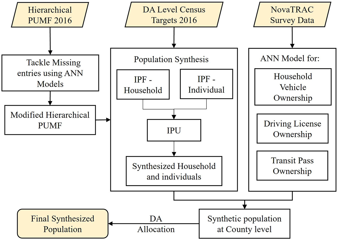
The process of population synthesis.

Firstly, the missing entries in the PUMF were input using an ANN model. Nearly 2% of the samples are missing gender attributes, and 8.5% are missing age group attributes. Removing entries of the samples with unavailable entries for age and gender will reduce the sample size and affect the underlying distribution of the microdata, which will lead to a wrong synthetic population distribution. Removing those samples affects the individuals per household ratio in the microsample, and results in a reduced number of individuals synthesized, as the missing data is mostly present in households with higher numbers of members. Therefore, the missing age group and gender of the samples are estimated using an ANN model by learning from all Canada PUMFs. This modified file together with census county-level targets is used to develop the synthetic population at the county level. Although the PUMF poses a better overall and joint distribution of socio-demographic parameters, it does not include some of the key transport modeling-related attributes, such as household vehicle ownership, driver’s license ownership, and transit pass ownership. These attributes, including individual- and household-level attributes are collected under the NovaTRAC survey. As the PUMF poses a better overall and joint distribution of socio-demographic characteristics than the survey data it is not directly used as the microsample for the population synthesis process. A FNN method was used to learn these three attributes from the survey data and was applied to the synthetic population to expand the list of attributes available as the base-year synthetic data for the iTLE. The allocation of synthetic data to microspatial units is executed using a CMC simulation.

The developed population synthesizer took 12 min to produce the synthetic population using the zone-by-zone approach at the spatial unit of a county (18 counties) with an average of 40 s per zone on a 32 GB RAM, i7 13th-generation processor system. DA allocation took 2.25 h to allocate the households to 1593 DAs with a rate of 11.8 DAs per minute.

Iterative Proportionate Updating Algorithm

The IPU algorithm is an extension of the traditional IPF method; the algorithm was first presented by Ye et al. ( 13 ). The general IPU algorithm is designed to efficiently generate synthetic populations by matching both household- and person-level characteristics. The process begins by creating a frequency matrix D, which details the household types and the frequency of various person types within each household in the sample. This matrix has dimensions N×m, where N is the number of households and m is the number of population characteristic constraints. Each element d_{i
j} in the matrix represents the contribution of household i to the frequency of population characteristic j. Next, joint distributions of household and person type constraints are calculated using the standard IPF procedure, and the resulting estimates are stored in a column vector C. Initial weights W are set to 1 for all households, and a scalar ϵ_min is initialized to a small positive value. The algorithm then iteratively adjusts the weights. For each constraint, it identifies the indices of non-zero elements in the corresponding column, calculates an adjustment factor α, and updates the weights for the households contributing to the constraint. This process is repeated for all constraints. After adjusting the weights for all constraints, the algorithm calculates a goodness-of-fit metric to measure how well the current weights match the desired population characteristics. If the change in this metric is smaller than a predefined threshold, the algorithm updates ϵ_min and stores the current weights as the best solution so far. The iteration counter is then incremented, and the process repeats until convergence is achieved, indicated by a minimal change in the goodness-of-fit metric. The final weights, which correspond to the smallest absolute relative difference ϵ_min, are stored as the solution:

ϵ = \frac{\sum_{j} [(\sum_{i} d_{i, j} \times w_{i} - c_{j}) / c_{j}]}{m}

(1)

After updating the household weights, they are recorded in the column vector SW. In this algorithm the value of ϵ is not always strictly decreasing, making it necessary to ensure that weights corresponding to the minimum value of ϵ are retained at each iteration. On concluding the process, a final solution is obtained if it falls within the feasible range. If the solution is not attainable, additional steps are taken to choose an appropriate corner solution, ensuring that household constraints are perfectly met. These steps involve iteratively adjusting the weights for household constraints. Starting with initializing a scalar h, the indices of non-zero elements for each household constraint are retrieved, adjustments are calculated, and weights are updated accordingly. This process is repeated until all household constraints are satisfied, reaching a corner solution and terminating the algorithm ( 13 , 14 ).

Microspatial Allocation of the Synthesized Population

The allocation of synthetic data to microspatial units is executed using a CMC simulation. Figure 3 shows the CMC process developed for the allocation. The process begins by drawing a pool of candidate households from the total sample. If a DA lacks households in a specific category (e.g., dwelling type = apartment), samples with that attribute are excluded from the draw. This sampling occurs incrementally, ensuring the ratio of each category within the DA is matched. Initially, a sample pool is drawn to match income distribution in the DA. Subsequently, the samples are drawn to matches the ratios of three other household-level attributes, one by one. The samples from these four steps are then combined to form a representative sample for the specific DA. Next, a random draw is performed from this representative sample to match the total number of households in the zone. The errors between the drawn sample and actual DA targets—such as the total number of members in the DA, gender distribution (male), and income class distribution (>C$100,000)—are estimated and recorded. This process is iterative: a random draw is performed, and if the new sample reduces the error, it replaces the previous sample; otherwise, another draw is conducted. This iterative process continues for a high number of iterations (e.g., 1000–2000), and it terminates either when a satisfactory error percentage (0.1%) is achieved for all three target attributes or when the maximum number of iterations is reached.

Figure 3.

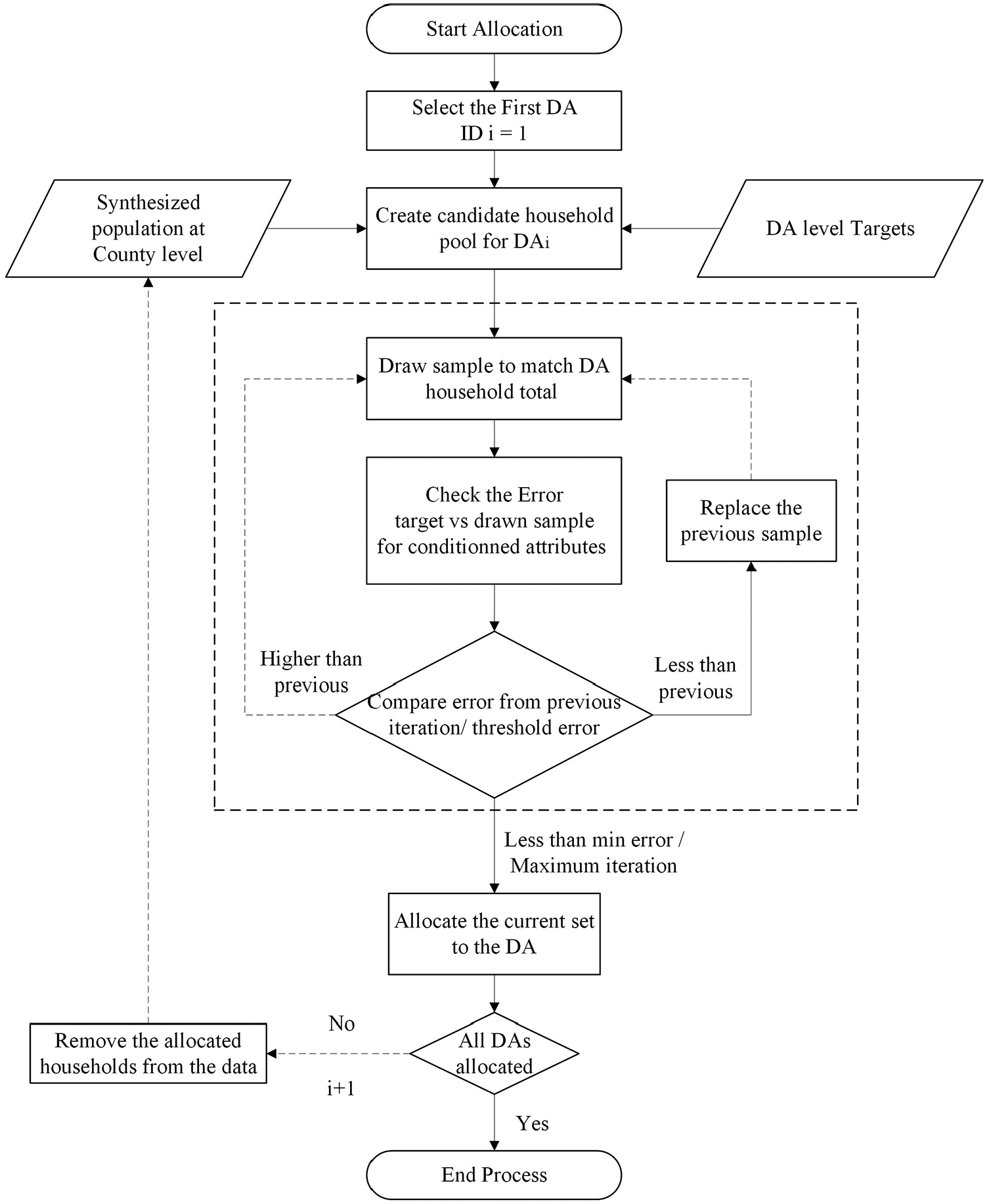
Microspatial allocation of households.

Feedforward Neural Network

Neural networks are non-linear statistical models that can be utilized for regression and classification tasks in machine learning applications. The FNN, also known as a multilayer perceptron (MLP), was used in this study to estimate household vehicle ownership, individuals' driver’s license ownership, and transit pass ownership. The neural network was trained using data from the NovaTRAC survey and applied to the synthetic population.

Theoretical Framework

The FNN consists of an input layer, one or more hidden layers, and an output layer. Each layer comprises neurons that process input data through weighted connections (refer to Figure 4).

Figure 4.

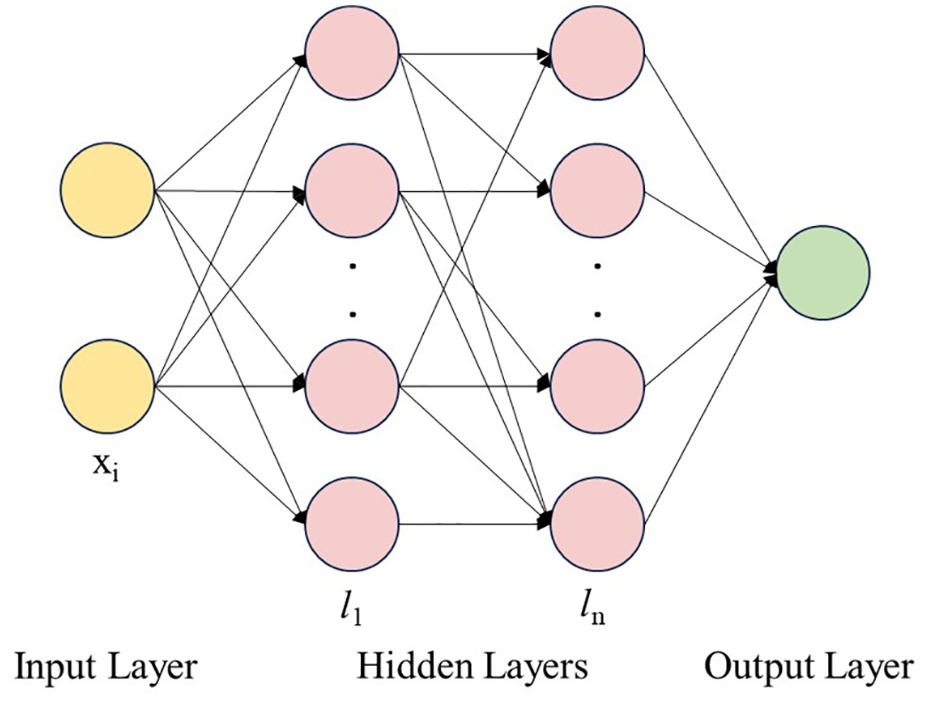
Artificial neural network structure.

Let x = [x₁, x₂, …, x_n] represent the input vector where x_i are the features of the input data. Each hidden layer l consists of neurons that perform a weighted sum of their inputs and pass this sum through an activation function. The output of the j neuron in layer l is given by the following:

z_{j}^{l} = \sum_{i} w_{ij}^{l - 1} a_{i}^{l - 1} + b_{j}^{l}

(2)

where $w_{ij}^{l - 1}$ is the weight from the ith neuron in layer l−1 to the jth neuron in layer l, $a_{i}^{l - 1}$ is the activation function of the ith neuron in layer l−1, and $b_{j}^{l}$ is the basis for the jth neuron in layer l.

The activation $a_{j}^{l}$ of the jth neuron in layer l is obtained by applying an activation function f to $z_{j}^{l}$ . A rectified linear unit (ReLU) activation function is used in this study. The final hidden layer’s outputs are passed to the output layer, where each neuron k in the output layer produces an output $o_{k} = a_{k}^{L}$ , where L is the index of the final hidden layer. For regression tasks, the output layer is typically assigned a linear activation function, and for classification a softmax activation function is used. Subsequently, the output is compared with the target values using a loss function L; a cross-entropy loss function is used for this study:

L = - \frac{1}{N} \sum_{i = 1}^{N} \sum_{k = 1}^{K} y_{i, k \log ({\hat{y}}_{i, k})}

(3)

where $y_{i, k}$ is a binary indicator if class label k is the correct classification for sample i and ${\hat{y}}_{i, k}$ is the predicted probability of sample i being in class k.

The final step in the process is backpropagation and optimization. The backpropagation algorithm is used to minimize the loss function. The gradients of the loss function for each weight and bias are computed using the chain rule of calculus. These gradients are then used to update the weights and biases. Common optimization algorithms include stochastic gradient descent (SGD) and Adam ( 33 ).

The dataset is first divided into a training set (80% of the entries) and a testing set (20%). Before training the model, the data were normalized as per a Gaussian distribution:

\hat{x} = \frac{X - μ_{X}}{σ_{X}}

(4)

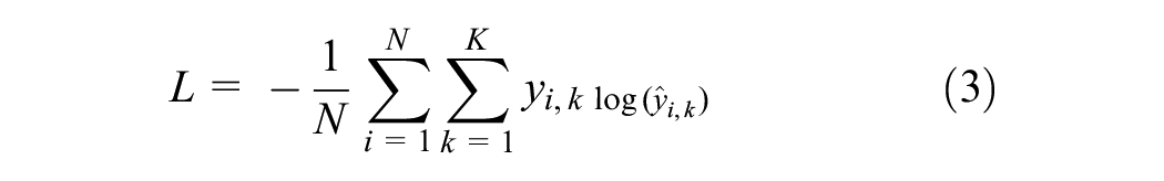
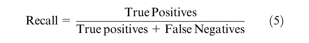
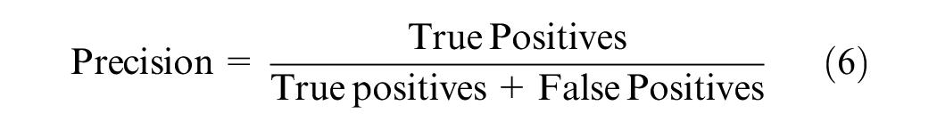
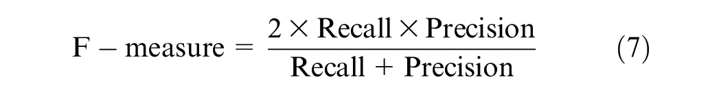
Testing accuracy and the confusion matrix are the most common measurements to evaluate machine learning models' prediction accuracy. Although the testing accuracy is a useful overall indicator, it assumes equal weight for both false positives and false negatives. Therefore, in addition, several other measures, such as recall, precision, and the F-measure, were also considered to test the accuracy ( 28 ). A high recall indicates that the class is accurately identified, resulting in a small number of false negatives. A high precision indicates that the class is accurately predicted with a lesser number of false positives:

Recall = \frac{True Positives}{True positives + False Negatives}

(5)

Precision = \frac{True Positives}{True positives + False Positives}

(6)

F - measure = \frac{2 \times Recall \times Precision}{Recall + Precision}

(7)

Mobility Tool Ownership Model Specifications

Three FNN models were developed from the NovaTRAC data to estimate the household vehicle ownership, individual-level driver’s license, and transit pass ownership. For household-level vehicle ownership, the input layer includes household income, dwelling type, tenure type, number of members in the household, number of workers in the household, and number of members under the age of 15. To achieve maximum testing accuracy, different combinations of the number of hidden layers and neurons were tested, and the final architecture consisted of three hidden layers with 40 neurons each, using ReLU activation functions, followed by an output layer with a softmax activation function for multi-class classification. For individual-level driver’s license and transit pass ownership, the input layer includes age, gender, household income, household size, dwelling type, tenure type, number of workers in the household, and number of children in household attributes. The final models included three hidden layers with 30 neurons each, using ReLU activation functions. A sigmoid activation function was applied in the output layer for binary classification. In addition, class weights were calculated and applied during training to address the class imbalance and improve sensitivity to underrepresented classes.

Results

The results section of the paper is subdivided into three parts. Firstly, the efficiency of enhancing the PUMF data by inputting the missing data in the PUMF using an ANN model is discussed. The next section presents the population synthesis results and error comparison of the whole study area (Nova Scotia) at a micro spatial level (DA). Finally, the mobility tool ownership results from neural network models are discussed, and the vehicle ownership results are validated.

Missing Data in the PUMF

The PUMF has detailed socio-demographic information of 4020 households and 9076 individuals in Nova Scotia. Out of these entries, a gender attribute is not available for 178 entries (2% of the sample) and the age group attribute is not available for 768 samples (8.5% of the sample), whereas other targeted variables are missing only for <0.1% of the samples. The ANN model utilized the employment status, marital status, income, education level, census family status, primary household maintainer, and number of members in the household as input variables to learn the age and gender of a person. For gender an overall testing accuracy of 73% was achieved. For the age group, 68% of testing accuracy was achieved with 82% of the predictions falling within +/−1 age group categories. The treated PUMF yields better distribution against the census target totals compared to the PUMF data with removed samples with missing values. Figure 5 shows the deviation of PUMF distribution against the census totals for both cases.

Figure 5.

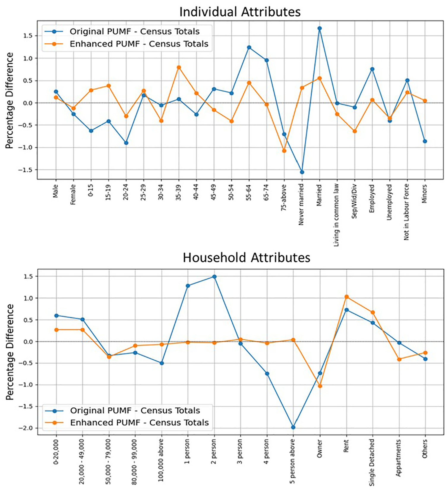
Comparison of the treated public use microdata file (PUMF) and original PUMF after deleting samples with missing entries.

Population Synthesis Results

Utilizing the weights generated from the IPU process a 100% synthetic population was developed for the Nova Scotia region. A total of 922,745 individuals were generated using the population synthesis process. Compared to the actual population of 922,070, the synthesized population is slightly higher with an error percentage of 0.07%. Among the household-level attributes, household income less than C$ 20,000 has the highest error percentage with −0.77%, followed by the household size of 5 people plus, which poses a 0.65% error, and dwelling type “others,” which poses a −0.65% error. All the other household categories have an error percentage from −0.5% to +0.5%. Among the individual-level attributes, the age group “40–44” has the highest error percentage of 1.05%, followed by the age group “15–19” with 0.84%, the age group “0–14” with −0.77%, and the age group “50–54” with 0.56% error. All the other individual categories have an error percentage from −0.5% to +0.5%. The age group categories posing a slightly higher error could be because of the higher number of categories (12 age group categories) included compared with other attributes. The comparison of census target totals and synthesized population totals for each category is presented in Figure 6. Household-level attributes show an average root mean square error (RMSE) of 170 households (0.04%) and an average RMSE of 652 individuals (0.07%) for individual-level attributes.

Figure 6.

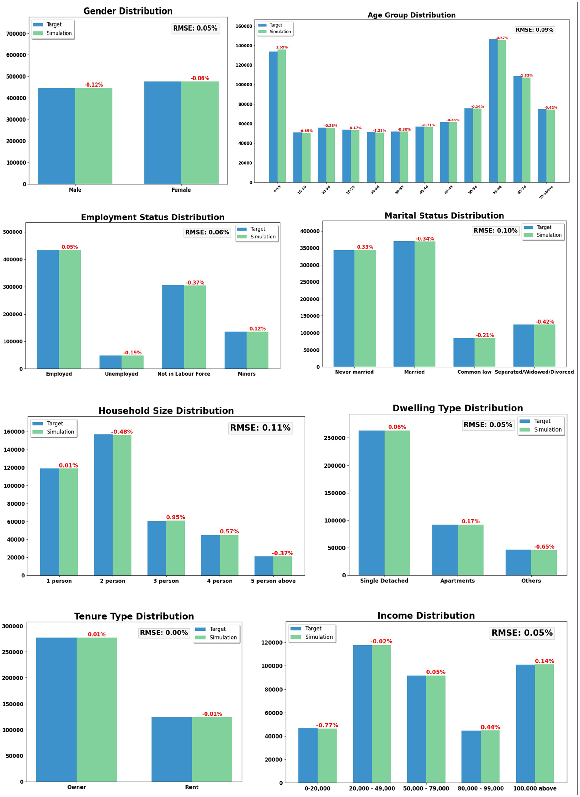
Comparison of census versus synthesized population totals.

To assess the joint distribution of the synthetic population, it is compared with the joint distribution of the PUMF data. Joint distribution of the synthetic data pool’s six individual-level attribute combinations (Gender × Age group, Gender × Marital status, Gender × Employment, Marital status × Age, Marital status × Employment, and Employment × Age) and six household-level combinations (Income × Number of Members, Income × Tenure, Income × Dwelling type, Number of members × Tenure, Number of members × Dwelling type, and Tenure × Dwelling type) was compared against the PUMF data joint distribution. The R² value of the Gender × Age distribution is the lowest with 0.96; almost all other distributions pose an R² value close to 1 (refer to Figure 7). This indicates that the joint distribution of the synthetic data closely matches with the actual distribution

Figure 7.

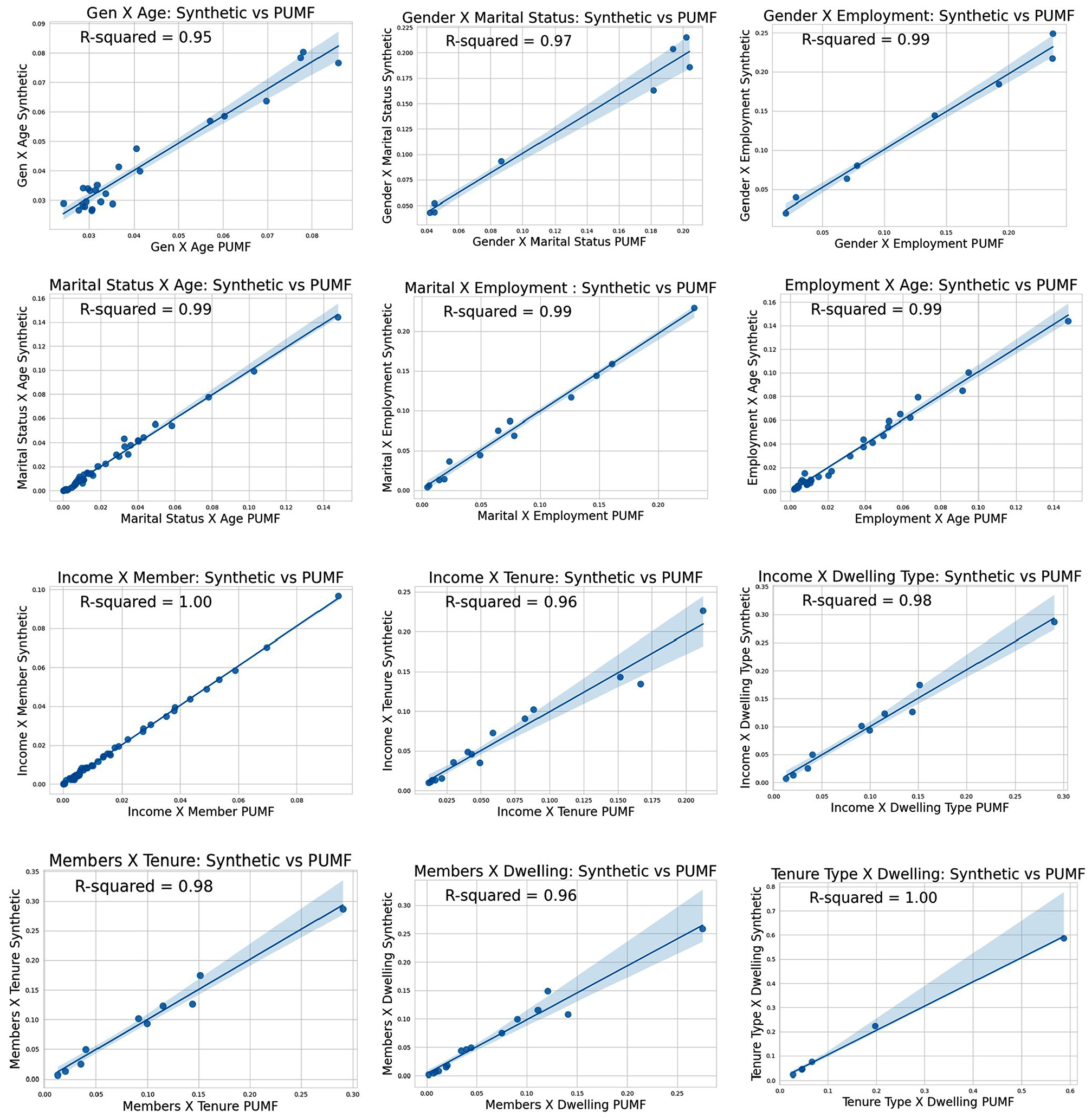
Joint distribution—synthetic versus public use microdata file (PUMF) data.

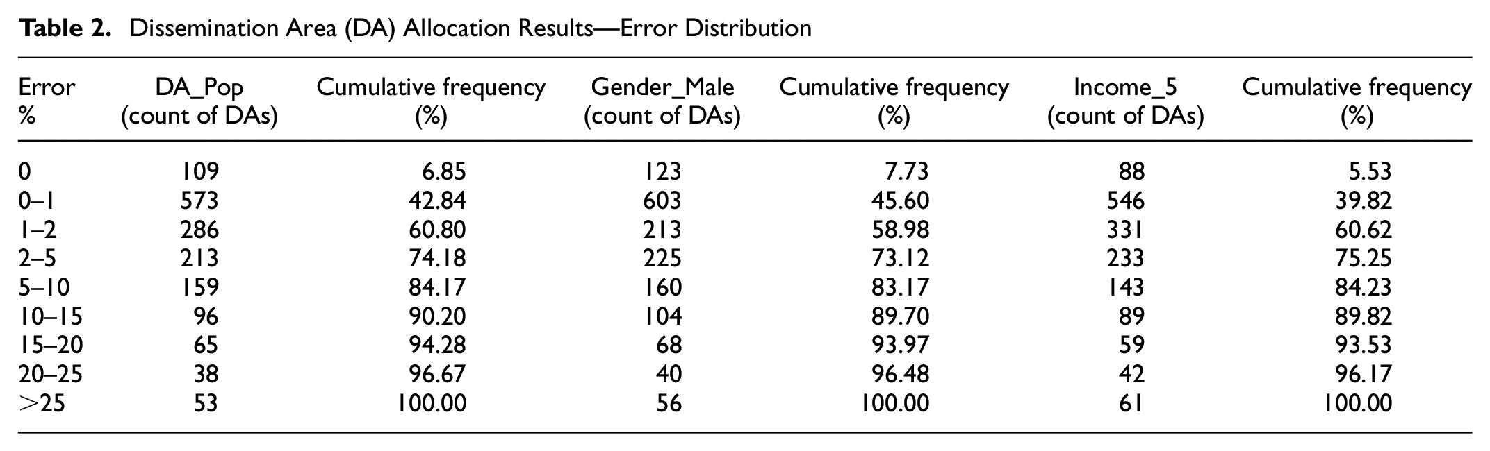
The error percentage distribution for allocating synthetic data into DAs is shown in Table 2. Some 74.2% of the DAs are allocated with a population within 5% error, whereas 84.2% of DAs are allocated withi <10% error and 96.7% of DAs with <25% error. Similarly, error distribution of gender (males) shows 73% of the DAs are allocated within 5% of error and 96.48% of the DAs are within 25% of error. For income category 5, 75.25% of DAs are allocated within 5% error, and 96.17% are allocated within 25% error. Moreover, the cumulative frequency distributions for population, gender (male), and income (Income_5) attributes show a similar trend, and they show consistency in synthetic data allocation across different demographic variables. Figure 8 shows the error in the microspatial distribution of DA population and gender.

Table 2.

Dissemination Area (DA) Allocation Results—Error Distribution

Error %	DA_Pop (count of DAs)	Cumulative frequency (%)	Gender_Male (count of DAs)	Cumulative frequency (%)	Income_5 (count of DAs)	Cumulative frequency (%)
0	109	6.85	123	7.73	88	5.53
0–1	573	42.84	603	45.60	546	39.82
1–2	286	60.80	213	58.98	331	60.62
2–5	213	74.18	225	73.12	233	75.25
5–10	159	84.17	160	83.17	143	84.23
10–15	96	90.20	104	89.70	89	89.82
15–20	65	94.28	68	93.97	59	93.53
20–25	38	96.67	40	96.48	42	96.17
>25	53	100.00	56	100.00	61	100.00

Figure 8.

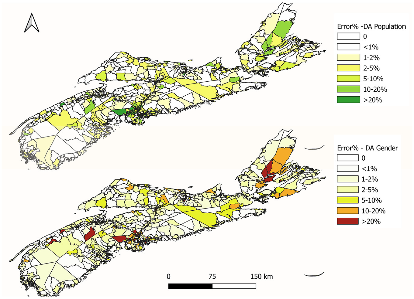
Error percentage: allocated population versus actual population.

Mobility Tool Ownership Results

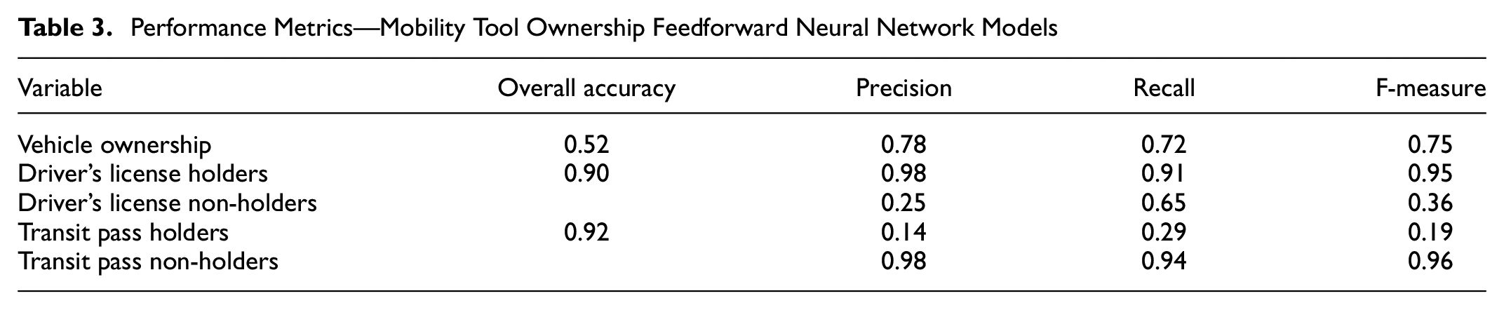
Table 3 presents performance metrics from the FNN model used to predict ownership attributes: number of vehicles owned by household, driver’s license ownership, and transit pass ownership of individuals. The metrics included are overall accuracy, precision, recall, and F-measure. The vehicle ownership model demonstrates an accuracy of 52% in predicting the exact number of vehicles owned and 87% of the predictions fall within +/−1 the number of vehicles owned. Precision for vehicle ownership is 0.78, meaning 78% of those expected to own vehicles do own them. The recall of 0.72 indicates that the model identifies 72% of actual vehicle owners with the exact number of vehicles they own. The F-measure is 0.75, demonstrating a reasonable balance between precision and recall. Figure 9a shows the test results confusion matrix of the vehicle ownership model.

Table 3.

Performance Metrics—Mobility Tool Ownership Feedforward Neural Network Models

Variable	Overall accuracy	Precision	Recall	F-measure
Vehicle ownership	0.52	0.78	0.72	0.75
Driver’s license holders	0.90	0.98	0.91	0.95
Driver’s license non-holders		0.25	0.65	0.36
Transit pass holders	0.92	0.14	0.29	0.19
Transit pass non-holders		0.98	0.94	0.96

Figure 9.

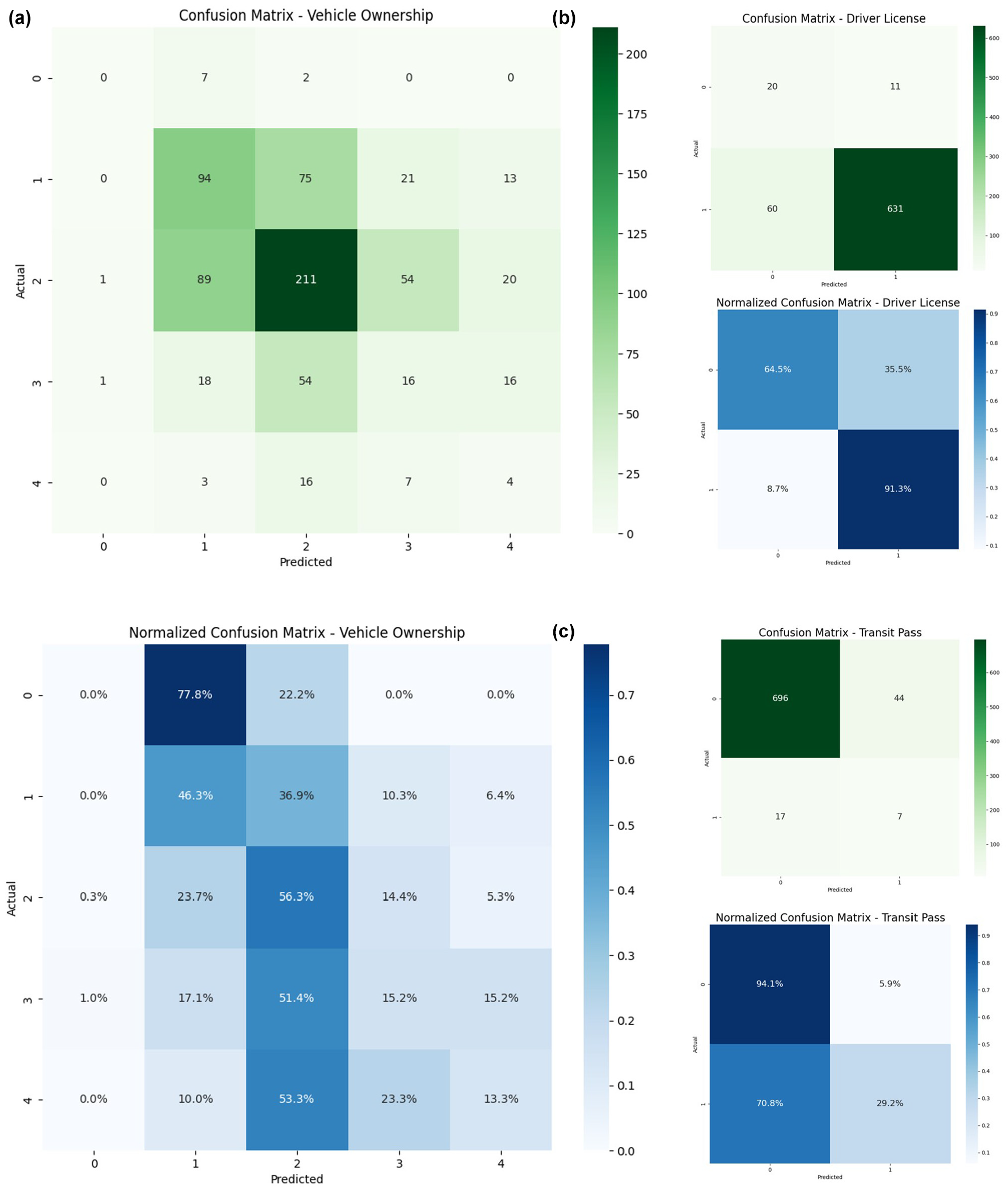
Confusion matrix— feedforward neural network model predictions: (a) Vehicle Ownership, (b) Driving License, and (c) Transit Pass.

The FNN model developed was applied to the synthetic population to estimate the three variables. Figure 10 shows the aggregated household vehicle ownership rate by income class and number of members in households. The model predicted a slightly higher vehicle ownership rate for income classes 4 and 5 and a lower rate for other income classes. The difference in the rate for all income classes is less than 0.2 vehicles per household. Also, the model results in a higher aggregated vehicle ownership rate for households with four members and a slightly lower rate for other classes. Overall, the model produced a better aggregate level of distribution with respect to household vehicle ownership, driver's license ownership, and transit pass ownership.

Figure 10.

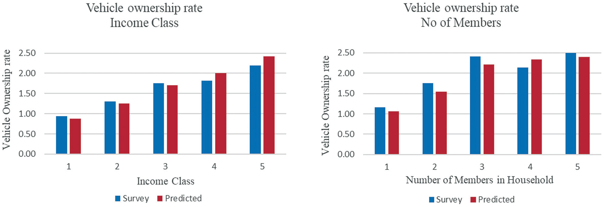
Household vehicle ownership rate by income class and number of members.

The comparatively lower individual-level accuracy in predicting the exact number of vehicles owned per household can be attributed to overlapping socio-demographic profiles among adjacent vehicle ownership classes (e.g., distinguishing between one- and two-vehicle households). In addition, as shown in the confusion matrix (Figure 9a), the model often predicts vehicle ownership within ±1 of the actual value, which is reasonable given the multi-class nature of the output. Despite these challenges, the aggregate-level predictions closely mirror the true distribution across income groups and household sizes (Figure 10), with deviations under 0.2 vehicles per household. This suggests that while the model may not always capture individual-level counts precisely, it performs well in maintaining the overall structure and distribution of vehicle ownership in the synthetic population, demonstrating its utility for aggregate travel demand modeling and agent-based simulation inputs.

The precision of 0.98 on driver’s license holders shows that 98% of the individuals who were identified to own driver’s licenses own a driver’s license. Also, 91% of the actual driver’s license holders are predicted to own a driver’s license. In contrast, the model's prediction of non-driver’s license holders is low compared to the prediction of driver’s license holders. The model accurately predicts 65% of the non-driver’s license holders and out of the predicted people without a driver’s license only 25% of them do not own a driver’s license. Some 98% of the non-transit pass owners are accurately predicted by the model and 94% of the people who are predicted not to own a transit pass do not own a transit pass in reality. The lower prediction accuracy for non-driver’s license holders and transit pass holders is primarily because of class imbalance. These groups represent a small share of the population, leading the model to be biased toward the majority class. When training data is skewed, the model receives limited examples to learn minority class patterns effectively. Figure 9, b and c, shows the test results confusion matrix of the two models.

Conclusions

This study aimed to develop a novel population synthesizer as a part of an agent-based iTLE and develop the base-year synthetic population for the province of Nova Scotia. A prototype iTLE is currently operational for HRM, one of the counties in Nova Scotia. However, the existing version of the model uses 2006 synthetic data as the base-year population, and the synthetic data developed in this study will update the baseline synthesis of the model. In addition, the synthetic population will be used as the base-year population data for a provincial-level travel demand model under development for Nova Scotia. The population synthesizer is equipped with the zone-by-zone IPU method to develop the synthetic data and a CMC simulation method to assign the synthetic data into micro spatial units, in this case, DA. The IPU method was selected as the method because of its accuracy and easy adaptability across geographies while advancing the iTLE for other regions.

Initially, the missing values of some samples in the PUMF data (age group and gender attributes) were input using a neural network model that learned the pattern from the nationwide PUMF. The enhanced PUMF data show a better distribution against census target totals compared to the PUMF with samples removed for missing entries. A total of 922,745 individuals were generated through the synthesis process, with a negligible population-level error of 0.07% compared to the actual Nova Scotia population. Most household-level variables had an error between −0.5% and +0.5%, except for income below C$20,000, household size over five, and dwelling type “others.” At the individual level, all categories had errors within ±0.5% except for four age groups. The synthetic population has a close enough joint distribution of individual and household characteristics with the PUMF data and shows an R² value close to 1 for all combinations. The synthesized population at the county level was allocated to the DAs using a Monte Carlo method with conditions on total households, population, gender (male), and income (class 5).

To add the base-year mobility tool ownership attributes for the synthesized agents, such as household vehicle ownership, driver’s license ownership, and transit pass ownership, a FNN model was developed from NovaTRAC survey data. The model predicted an overall accuracy of 52% for number of vehicles owned by a household with 87% of the prediction falling within +/−1 vehicle per household. The model demonstrates 90% overall testing accuracy in predicting driver’s license holders, and 92% in predicting transit pass owners. Even though the model showed greater overall accuracy in predicting driver’s license ownership and transit pass ownership, the model shows lower accuracy in predicting the non-driver’s license holders and transit pass holders as the share of these categories is very low in the dataset. The developed FNN model was applied to the synthetic population; the vehicle ownership rate of the synthetic population shows a close distribution to the survey data.

The current study uses a zone-by-zone approach with IPU for the synthesis and a conditional random allocation for microspatial units in which the unconditioned variables may not be accurately distributed to the microspatial units. Moreover, this allocation process is sequential, where the allocation of DAs happens in the order they are listed in the constraint file. The errors for the DAs at the bottom of the list show higher error percentages compared to the ones listed at the top. This has led to some DAs showing higher error percentages for all three constraint variables. This is mainly because after allocation, the households are removed from the pool, and the DAs at the bottom do not have sufficient samples to choose for a better fit. The developed synthesizer code will be updated to employ a multizone approach in the future to overcome this limitation. Generalized raking is another method widely used by researchers for allocation to microspatial units that can also be tested.

Although the IPU method shows greater accuracy in fitting, the distribution of the synthetic population greatly depends on the accuracy of the PUMF data distribution, and it is replicated in the final output. Future study is expected to incorporate deep generative learning algorithms such as generative adversarial networks (GANs) to produce synthetic data. One of the limitations of the study is that the FNN model could not predict transit pass owners accurately, as the number of observations in the dataset is too low for this class. Also, machine learning models lack interpretability and face difficulty in post-calibration compared to other econometric models. A hybrid framework could be developed by combining discrete choice models, which show greater interpretability, and machine learning models with greater predictive accuracy. Overall, the study developed a synthetic population for Nova Scotia with satisfactory accuracy and representativeness.

Footnotes

Author Contributions

The authors confirm contribution to the paper as follows: study conception and design: M.A. Habib, V. Arunakirinathan; data collection: M.A. Habib; analysis and interpretation of results: V. Arunakirinathan, M.A. Habib; draft manuscript preparation: V. Arunakirinathan, M.A. Habib. All authors reviewed the results and approved the final version of the manuscript.

Declaration of Conflicting Interests

The author(s) declared no potential conflicts of interest with respect to the research, authorship, and/or publication of this article.

Funding

The author(s) disclosed receipt of the following financial support for the research, authorship, and/or publication of this article: This work was supported by the Natural Sciences and Engineering Research Council (NSERC) Alliance, Grant No. ALLRP 577187-2022.

ORCID iDs

Vajeeran Arunakirinathan

Muhammad Ahsanul Habib

References

Briem

Mallig

Vortisch

Creating an Integrated Agent-Based Travel Demand Model by Combining mobiTopp and MATSim. The 8th International Workshop on Agent-Based Mobility, Traffic and Transportation Models, Leuven, 2019.

Fabrice Yaméogo

Gastineau

Hankach

Vandanjon

P. O.

Comparing Methods for Generating a Two-Layered Synthetic Population. Transportation Research Record: Journal of the Transportation Research Board, 2020. 2675: 136–147.

Habib

M. A.

McCarthy

Development of an Integrated Transportation and Land Use Microsimulation Model on a Flexible Modeling Platform. Transportation Research Record: Journal of the Transportation Research Board, 2021. 2675: 355–369.

Axhausen

K. W.

Müller

Population Synthesis for Microsimulation: State of the Art. ETH Library, https://doi.org/10.3929/ethz-a-006132973.

Deming

W. E.

Stephan

F. F.

On a Least Squares Adjustment of a Sampled Frequency Table When the Expected Marginal Totals Are Known. The Annals of Mathematical Statistics, Vol. 11, No. 4, 1940, pp. 427–444.

Beckman

R. J.

Baggerly

K. A.

McKay

M. D.

Creating Synthetic Baseline Populations. Transportation Research Part A: Policy and Practice, Vol. 30, No. 6, 1996, pp. 415–429..

Guo

J. Y.

Bhat

C. R.

Population Synthesis for Microsimulating Travel Behavior. Transportation Research Record: Journal of the Transportation Research Board, 2007. 2014: 92–101.

Auld

Mohammadian (Kouros)

M. A.

Waddell

K. W.

Population Synthesis with Subregion-Level Control Variable Aggregation. Journal of Transportation Engineering, Vol. 135, No. 9, 2009, pp. 632–639. https://doi.org/10.1061/(ASCE)TE.1943-5436.0000040.

Pritchard

D. R.

Miller

E. J.

Advances in Population Synthesis: Fitting Many Attributes per Agent and Fitting to Household and Person Margins Simultaneously. Transportation, Vol. 39, No. 3, 2012, pp. 685–704. https://doi.org/10.1007/s11116-011-9367-4

10.

Prédhumeau

Manley

A Synthetic Population for Agent-Based Modelling in Canada. Scientific Data, Vol. 10, No. 1, 2023. https://doi.org/10.1038/s41597-023-02030-4

11.

Arentze

Timmermans

Hofman

Creating Synthetic Household Populations: Problems and Approach. Transportation Research Record: Journal of the Transportation Research Board, 2007. 2014: 85–91.

12.

Zhu

Ferreira

Jr.

Synthetic Population Generation at Disaggregated Spatial Scales for Land Use and Transportation Microsimulation. Transportation Research Record: Journal of the Transportation Research Board, 2014. 2429: 168–177.

13.

Konduri

K. C.

Pendyala

R. M.

Sana

Methodology to Match Distributions of Both Household and Person Attributes in Generation of Synthetic Populations. Transportation Research Record: Journal of the Transportation Research Board, 2010. 2175: 212–221.

14.

Tian

Wang

F. Y.

On Iterative Proportional Updating: Limitations and Improvements for General Population Synthesis. IEEE Transactions on Cybernetics, Vol. 52, No. 3, 2022, pp. 1726–1735. https://doi.org/10.1109/TCYB.2020.2991427

15.

Voas

Williamson

An Evaluation of the Combinatorial Optimisation Approach to the Creation of Synthetic Microdata. International Journal of Population Geography, Vol. 6, No. 5, 2000, pp. 349–366. https://doi.org/10.1002/1099-1220(200009/10)6:5<349::AID-IJPG196>3.0.CO;2-5

16.

Voas

Williamson

Evaluating Goodness-of-Fit Measures for Synthetic Microdata. Geographical and Environmental Modelling, Vol. 5, No. 2, 2001, pp. 177–200. https://doi.org/10.1080/13615930120086078

17.

Hafezi

M. H.

Habib

M. A.

Synthesizing Population for Microsimulation-Based Integrated Transport Models Using Atlantic Canada Micro-Data. Transportation Research Record: Journal of the Transportation Research Board, 2014. 2429: 410–415.

18.

Farooq

Bierlaire

Hurtubia

Flötteröd

Simulation Based Population Synthesis. Transportation Research Part B: Methodological, Vol. 58, 2013, pp. 243–263. https://doi.org/10.1016/j.trb.2013.09.012

19.

Saadi

Mustafa

Teller

Farooq

Cools

Hidden Markov Model-Based Population Synthesis. Transportation Research Part B: Methodological, Vol. 90, 2016, pp. 1–21. https://doi.org/10.1016/j.trb.2016.04.007

20.

Rahman

M. N.

Fatmi

M. R.

Population Synthesis Accommodating Heterogeneity: A Bayesian Network and Generalized Raking Technique. Transportation Research Record: Journal of the Transportation Research Board, 2023. 2677: 41–57.

21.

Zhang

Cao

Feygin

Tang

Shen

Z.-J.

Pozdnoukhov

Connected Population Synthesis for Transportation Simulation. Transportation Research Part C: Emerging Technologies, Vol. 103, 2019, pp. 1–16. https://doi.org/10.1016/j.trc.2018.12.014.

22.

Ilahi

Axhausen

K. W.

Integrating Bayesian Network and Generalized Raking for Population Synthesis in Greater Jakarta. Regional Studies, Regional Science, Vol. 6, No. 1, 2019, pp. 623–636. https://doi.org/10.1080/21681376.2019.1687011

23.

Borysov

S. S.

Rich

Pereira

F. C.

How to Generate Micro-Agents? A Deep Generative Modeling Approach to Population Synthesis. Transportation Research Part C: Emerging Technologies, Vol. 106, 2019, pp. 73–97. https://doi.org/10.1016/j.trc.2019.07.006

24.

Püschel

Barthelmes

Kagerbauer

Vortisch

Comparison of Discrete Choice and Machine Learning Models for Simultaneous Modeling of Mobility Tool Ownership in Agent-Based Travel Demand Models. Transportation Research Record, 2004. 2678: 376–390.

25.

Hensher

D. A.

Ton

T. T.

A Comparison of the Predictive Potential of Artificial Neural Networks and Nested Logit Models for Commuter Mode Choice. Transportation Research Part E: Logistics and Transportation Review, Vol. 36, No. 3, 2000, pp. 155–172. https://doi.org/https://doi.org/10.1016/S1366-5545(99)00030-7

26.

Príncipe

J. C.

Euliano

N. R.

Lefebvre

W. C.

Neural and Adaptive Systems: Fundamentals through Simulations. Wiley, New York, 2000.

27.

Mohammadian

Miller

E. J.

Nested Logit Models and Artificial Neural Networks for Predicting Household Automobile Choices: Comparison of Performance. Transportation Research Record: Journal of the Transportation Research Board, 2002. 1807: 92–100.

28.

Basu

Ferreira

Understanding Household Vehicle Ownership in Singapore through a Comparison of Econometric and Machine Learning Models. Transportation Research Record: Journal of the Transportation Research Board, 2020. 2674: 1674–1693.

29.

Rajalakshmi

Mode Choice Modelling Based on Work Trips – Artificial Neural Network Model. In Proceedings of the International Conference on Energy and Environment (ICEE 2013), 12–14 December 2013, 2007.

30.

Dixon

Koukoura

Brand

Morgan

Bell

Spatially Disaggregated Car Ownership Prediction Using Deep Neural Networks. Future Transportation, Vol. 1, No. 1, 2021, pp. 113–133. https://doi.org/10.3390/futuretransp1010008

31.

Niculescu-Mizil

Caruana

Predicting Good Probabilities with Supervised Learning. Proceedings of the 22nd International Conference on Machine Learning (ICML '05), Association for Computing Machinery, New York, NY, 2005, pp. 625–632. https://doi.org/10.1145/1102351.1102430.

32.

Fatmi

M. R.

Development of Integrated Urban System Models: Population Life-Transitions, Household Location, and Vehicle Transaction Decisions. Ph.D. dissertation, University of Toronto, 2017.

33.

Kingma

D. P.

Adam: A Method for Stochastic Optimization. arXiv preprint, arXiv:1412.6980, 2014.

Development of a Synthetic Population and its Baseline Mobility Tool Ownership for the Province of Nova Scotia

Abstract

Keywords

Literature Review

Population Synthesis Methods

Mobility Tool Ownership Modeling

Data Source

Methodology

Iterative Proportionate Updating Algorithm

Microspatial Allocation of the Synthesized Population

Feedforward Neural Network

Theoretical Framework

Mobility Tool Ownership Model Specifications

Results

Missing Data in the PUMF

Population Synthesis Results

Mobility Tool Ownership Results

Conclusions

Footnotes

Author Contributions

Declaration of Conflicting Interests

Funding

ORCID iDs

References