
Abstract
OpenStreetMap (OSM) data are geographical data that are easy and open to access and therefore used for a large set of applications including travel demand modeling. However, often there is a limited awareness about the shortcomings of volunteered geographic information data, such as OSM. One important issue for the application in travel demand modeling is the completeness of OSM elements, particularly points of interest (POI), since it directly influences the predictions of trip distributions. This might cause unreliable model sensitivities and end up in wrong predictions leading to expensive misinterpretations of the effects of policy measures. Because of a lack of large-scale real-world data, a detailed assessment of the quality of POI from OSM has not been done yet. Therefore, in this work, we assess the quality of POI from OSM for use within travel demand models using surveyed real-world data from 49 areas in Germany. We perform a descriptive and a model-based analysis using spatial, demographic, and intrinsic indicators for two common trip purpose categories used in travel demand modeling. We show that the completeness of POI data in OSM depends on the category of POI. We further show that intrinsic indicators and indicators calculated based on data from other sources (e.g., land use or census data) are able to detect quality deficiencies of OSM data.
Keywords
Travel demand models are essential tools to estimate the impacts of transport policy and infrastructure measures, since they are capable of simulating and assessing different scenarios. The results form the basis of extensive and usually costly decisions. The models must therefore be as accurate as possible in their forecasts. Therefore, they aim to simulate the travel behavior of people on the basis of several decisions: which activities are conducted, where the activities take place, and which means of transport and which routes are used on the trips. Choosing the destination of a trip is based on locations, where activities can be carried out: for example, supermarkets for grocery shopping, sports facilities for recreation, or train stations to pick up or drop off friends or relatives, to name a few.
Consequently, the structure of an area with different offerings contributes significantly to its attractiveness for a certain activity. Attractiveness is thus a structural parameter that forms the basis for modeling destination choice. This requires the collection of structural data, for example, retail facilities or cultural offerings. The data should be as detailed and up-to-date as possible. This type of data can be laboriously collected manually with the inclusion of existing surveys and official data. In addition, there are offers from commercial providers, which sell the data for accessibility analyses and market analyses, among other things. Accordingly, these offers cost money and the approach of the providers is not comprehensible.
At this point, open data offer several advantages. The data are provided in an open format that is usually well documented. This significantly reduces the effort for using the data from a technical perspective. If the data are available in a uniform format for different areas, any methods, frameworks, and procedures based on it can be easily transferred to other regions. Also, because the data are in a defined format, it can be processed automatically in all available areas. Furthermore, if the data are updated regularly, all models built on it can also be updated on a regular base. The public availability of the data also promotes transparency of the respective models. Everyone who knows the process can reproduce the results. Thus, there is no longer a “black box” as with most commercial data. One of the largest providers of geographical open data is OpenStreetMap (OSM), which belongs to the field of volunteered geographic information (VGI). VGI characterizes information collected by so-called “mappers” in their spare time and made available on platforms such as OSM.
Haklay points out that “volunteers…collect information of their own accord without top-down coordination that would ensure systematic coverage” ( 1 ). This raises the concern of points of interest (POI) not being equally complete in all areas, which would distort the destination choice. To use OSM data for travel demand modeling without hesitation, it is crucial to ensure comparably good-quality POI data for the designated areas.
Therefore, investigating whether POI related to certain activity types are mapped completely in the region of interest is of high relevance. Because of a lack of open or surveyed large-scale data from real-world POI, such an investigation is usually not feasible. However, there exist several approaches using intrinsic indicators, such as the historic saturation rate or the number of volunteers in a certain area. However, these intrinsic methods have also not been verified with real-world data so far for the same reasons. Therefore, in our work, we use surveyed data from real-world POI from 49 survey sites to: 1) perform an analysis of the completeness of POI data from OSM, 2) assess influences from spatial structures, and 3) evaluate the explanatory power of intrinsic indicators.
The paper is structured as follows. First of all, literature is reviewed for the present state of knowledge on POI data quality and requirements. The next section describes the data sources and the data processing as well as the calculation of the various indicators. This is followed by a section providing insights into the analysis methods and the results of our analysis. Finally, a summary of the work and an outlook is provided.
Literature
There are related national guidelines for the setup of travel demand models, which specify the requirements for different model aspects and input data. However, the use of structural data such as POI for different purposes is only of minor importance. Most of these guidelines—for example, the Swiss and British guidelines for data sources of travel demand models—only provide ideas for the use of POI data, and merely focus on the network data and related data of transport infrastructure such as time tables or stations ( 2 , 3 ).
Nevertheless the use, quality, and application of crowd-sourced POI data has been subject to a wide range of research. Depending on the purpose of an analysis, different dimensions of data quality are of concern ( 4 ). For the purpose of travel demand estimation, object completeness and correct classification of POI are of high importance while for navigation, correctness of topological relations plays as important role as well. Correctness of the geometrical representation (single point or floor area of buildings) of the object is of lower importance. Yeow et al. compared various measures and validation methods to assess POI data quality ( 5 ). They considered both intrinsic and extrinsic approaches and found positional accuracy to be the most-studied element of data quality. Thematic accuracy and completeness were less represented in the studies. As a measure of completeness, the share of observed POI compared with a reference database was the most popular one, whereas community activity can serve as an indicator as well. The completeness of POI data in the application area in Singapore was found to be weak suggesting “errors of commission and omission.” Hochmair et al. compares different sources of publicly available POI data of mapping and social media platforms without a comparison of ground truth data ( 6 ). The data of mapping platforms had a higher spatial accuracy than social media data. The authors proposed a closer look at POI contribution patterns and a further investigation of selected test areas. Touya et al. conducted a completeness and accuracy analysis based on a reference dataset and Flickr photographs, and highlighted the use of multiple indicators as each of them revealed strengths and weaknesses when applied to different POI categories ( 7 ).
Going beyond only looking at measures, influences such as spatial structure, demography, and community indicators on the data quality are of interest. Yang et al. analyzed positional accuracy and completeness of Chinese POI data and explored influencing factors by applying a geographically weighted regression ( 8 ). The distribution of the contributors was found to be most important, while population density and per capita GDP had little influence. Still, with respect to OSM data quality, many authors reported a tendency for higher data quality in more densely populated areas ( 1 , 8 , 9 ).
In general, one can find many approaches and research on how crowd-sourced POI data already in the database can be improved. Goodchild and Li describe approaches from involving local collaborations to geographical consistency checks integrated in the database to rely on correction through the crowd ( 10 ). Tré et al. provides a cleansing technique for checking coreferent POI ( 11 ).
Quality assessment of POI is already a popular subject in the field of geo-information. The approaches still barely focus on the completeness of POI and, if so, they focus on intrinsic assessments or the comparison of different sources of VGI. Completeness comparison with “ground truth data” is found only in a few cases and in geographically and POI type limited applications. Furthermore, data quality is highly dependent on the local community, leading to different results in quality assessment. A large-scale quality assessment with real-world data can therefore enable further insights into the usability of VGI data.
To date, no analysis on the completeness of POI in OSM based on a large-scale reference data set has been conducted. Therefore, based on surveyed data collected on various sites all over Germany, we aim to analyze factors which determine the completeness of OSM POI. To build the bridge to existing research using intrinsic assessments, we also include intrinsic features in our analysis to assess based on the extrinsic reference data if they are able to account for completeness as well.
Data
The aim of this research is to validate the completeness of POI data mapped in OSM. In this paper, we focus on POI for the two trip purposes shopping and private business since we focused on one activity with highly visible POI and one activity with rather hidden POI. For this purpose, relevant POI were extracted from OSM for the two activities using a tag filter defined in previous work ( 12 ). The extracted POI were then compared with real POI data from 49 areas, which were surveyed manually on site. In our analysis, we first compared the two data sets showing the absolute and relative difference. Then, we performed a mode-based analysis with the goal to explore dependencies between the deviation of OSM POI and external factors. Therefore, various indicators and features were calculated and engineered for all areas.
We then set up the hypothesis that the small size of the surveyed area might be too individual to explain correlations. Therefore, indicators and features were also calculated for the surroundings of the areas for a buffer of 0.5 km, 1.0 km, and 2.5 km as well as for the municipal level. The goal is to find out whether some indicators have an extraordinary influence which would lead to a structural distortion of the destination choice. In the following subsections, the preparation of the data and the indicators is described.
Ground Truth Data
To extrinsically validate the OSM data, we manually located POI in 49 survey areas throughout Germany. These survey areas are located in 17 mostly larger cities such as Dresden, Hamburg, or Munich. Nevertheless, survey areas in smaller cities close to these larger cities are also part of the ground truth data. However, even these smaller cities are predominantly located in urban regions (see Figure 1). The data collection was conducted as part of the project Cities in Charge, in which charging infrastructure for electric vehicles is planned, built, and evaluated. Therefore, the survey areas are located in the vicinity of the built charging infrastructure and include different types of neighborhoods from the city center to the outskirts (see the Descriptive Analysis section). To maximize the number of observations, cities with multiple charging infrastructures in the project were predominantly selected for data collection. We catalogued each externally visible POI into different survey categories in a census-grid-based near-circular area with a size of 37 ha surrounding the charging infrastructure. The resulting buffer has a radius of approx. 350 m. In a case where a POI could be assigned to multiple survey categories, we catalogued that POI in each assignable category. Data collection was conducted once per survey area between October 2019 and September 2021 and took between 20 min and 3 h for each survey area, depending on the density of the street network and the number of POI.
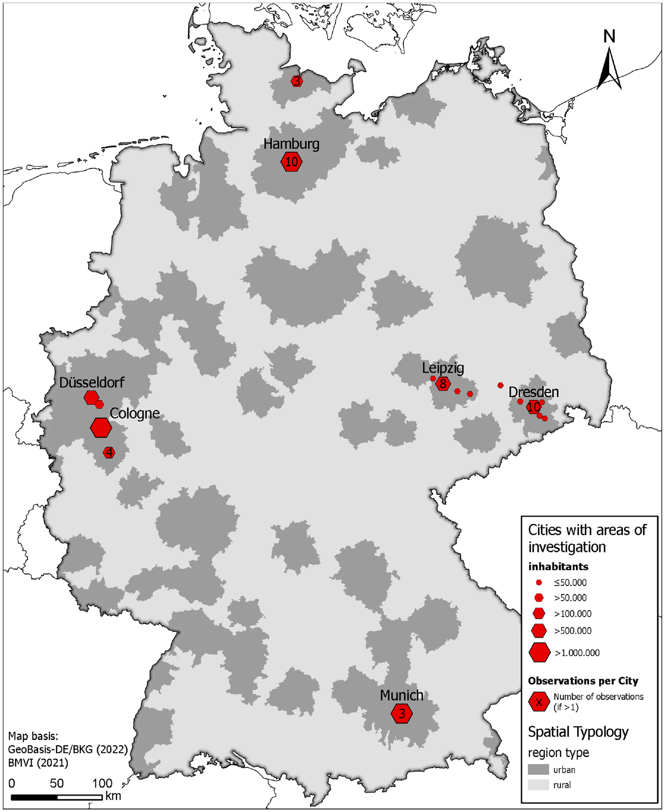
Map of the cities where the areas of investigation are located.
Data Preparation
We want to investigate the deviation between the number of OSM POI and real-world POI: we aim to find interrelations to be able to explain the deviation. Therefore, we first calculate features based on open data which describe the spatial context of the survey sites (e.g., land use data) on the one hand and intrinsic OSM data measures on the other hand.
Since the calculated indicators differ in spatial granularity, we calculated them for different areas surrounding the survey site to investigate on which granularity each feature is most significant. Overall, we calculated the features for the survey site area, a 0.5 km, 1.0 km, and 2.5 km buffer around the centroid of the survey site as well as for the municipality the survey site was in.
OSM POI Data
The corresponding state of the OSM database at the time of the survey was extracted by querying the OSM history database (OSHDB) using the ohsome API (https://api.ohsome.org) ( 13 ). The result of the queries is the total number of elements for each retrieved tag in the survey areas at the point of time of the site visit. Table 1 shows an example of the tag list used for the activity “private business.” It shows that many very different POI need to be assigned to a single activity of a travel demand model. The resulting data set consists of OSM POI for all areas of investigation for the activities private business and shopping.
Tag List for the Activity Type Private Business

Contributor Indicator
The number of active contributors in the respective area, the 1 km buffer, and the 2.5 km buffer were used as an intrinsic indicator. We calculated two variants: the number of all contributors and the number of contributors who dealt with POI. The hypothesis was that higher OSM contributor activity is associated with higher POI completeness.
POI Densities
POI densities per square kilometer for the most common activities in each area were calculated based on the OSM taglists developed in Klinkhardt et al. for all spatial levels ( 12 ).
Land Cover Data
Land use and land cover data derived from the European Copernicus programme—CORINE Land Cover (CLC)—were used to calculate the shares of land usage ( 14 ). CLC is the best-known European database on land use. It has been in use since 1990 and has been regularly updated and validated ( 15 ). For this examination, CLC 2018 is used. We aggregated the original categories of the CLC data to areas of similar land use (continuous urban fabric, discontinuous urban fabric, industrial or commercial units, transport, construction sites, green urban areas, sport and leisure facilities, agriculture, forest, nature, other). More details on the land use categories can be found in the CLC technical documentation ( 16 ). Since the categories continous urban fabric and discontinous urban fabric were strongly correlated in our data, we aggregated them to a new category urban fabric.
Official Data
Using official data from the 2011 German census, we were able to determine the population, dwellings and buildings in the areas of investigation ( 17 ). For this purpose we aggregated the 1 ha information for all census grids inside the areas of investigation. Furthermore, we used the 1 km × 1 km grid level to determine the number of inhabitants on a higher level and the age composition of the population. In addition, the population density was calculated at the level of zip codes. The Regional Statistical Spatial Typology for Mobility and Transport Research of the Federal Ministry of Transport and Digital Infrastructure Germany was used as additional governmental data.
Manually Created Indicators for Describing the Location
Some influencing factors could not be calculated, whereas a qualitative description of the survey areas was conducted. The distance from the centroid of the survey area to the nearest city center was measured. Also, the location in the city was qualitatively assessed using several categories. In addition, the building structure was classified into several categories.
Saturation Indicator
OSHDB stores the complete history of OSM, allowing to follow OSM contributions over time. The underlying assumption is that, for a specific category and region, contributions converge against the number of real-world objects in the area, given a sufficient OSM contributor activity. Saturation curves can be used to estimate the saturation level which represents an estimator for the true number of objects in a region.
Monthly counts of POI of the different categories were extracted from OSM using the ohsome API (https://api.ohsome.org) to query OSHDB for the time frame October 8, 2007, until May 29, 2022 ( 13 ). The same filter as in the collection of the POI data was used (i.e., 1). We followed an approach similar to Brückner et al. and fitted various limited growth curves to the OSM history for each survey area and estimated the completeness level via their saturation parameter ( 18 ). The curves used originate from two families: the three and four parameter logistic function (Equations 1 and 2), that belong to the sigmoid curve family as well as the rectangular hyperbola (Equation 3) and the asymptotic function (Equation 4) that belong to the non-logistic growth curves family. The family of sigmoid curves is suitable for a three-phase mapping process as also described by Barrington-Leigh and Millard-Ball ( 19 ). Curves of the non-logistic growth curves family tend to represent a mapping process without the initial phase of slow growth.


where
The curves were fitted separately for each of the POI categories. The reliability of the estimated asymptotes by the four functions was checked by several tests. We checked for an overall decline in growth, which is a fundamental criterion to estimate a saturation level as a proxy for the number of retail stores. Fitted models were filtered for unrealistic fits where the asymptote was estimated to be lower than the current number of POI of the category in OSM. To also account for the uncertainty of the models, we accepted fits with an asymptote at most 2% lower than the actual latest amount. In addition to the non-linear least square fit we also tested robust methods for all four types of the saturation curve. We used an M-estimator for the robust versions. We chose the best-fitting functional form of all accepted curves for each spatial unit based on the AIC. The completeness level was estimated as the quotient of the current number of retail stores and the asymptote of the estimated saturation curve.
As saturation curves can presumably be estimated more reliably for larger areas with more real-world objects, we also applied the saturation estimation for different buffer sizes around the original location polygons: 0.5 km, 1 km, and 2.5 km were explored. While saturation curve fitting can be assumed to be more reliable, this trades off with representativeness for the survey areas.
The analysis was performed in R, using the packages: ohsome (https://github.com/GIScience/ohsome-r), robustbase, sf, geojsonsf, tidyverse, ggplot2, and ggpubr ( 20 – 26 ).
Analysis
Having calculated the features mentioned before, we then compared the surveyed and the OSM POI data for the activities shopping and private business. For this, we used the count of POI, the relative deviation of OSM POI compared with real-world POI, and the difference of OSM POI compared with real-world POI as response variables. In the following, we will first compare the counted OSM POI descriptively with the surveyed POI. This is followed by several model-based approaches to reveal structural influences on POI completeness.
Descriptive Analysis
In total, 1,305 POI of the activity private business were counted on site in contrast to 292 POI in OSM. Consequently, only 22% of the locations were mapped, on average. The situation was better for the activity shopping. Here, 379 POI were present on site and 277 POI in OSM, which led to a completeness of 73%. These differences between activities can also be observed in Figure 2. Based on linear regression, we calculated balance lines for both graphs. The gradient for shopping was much steeper and thus much closer to the bisector on which all points would lie with complete OSM data. It can also be seen that private business was not only more incomplete, but also subject to much greater dispersion. One reason for this is that POI for shopping are usually highly visible to the outside to attract walk-in customers. Also, the volume of customers at POI associated with shopping is usually higher than at POI associated with private business. These observations can also be quantified. As a result of the linear regression, we find that for every private business POI in OSM there are 4.1786 POI in the real world with a standard error of 0.48 and a p-value of 3.028e-11. For shopping the value is 1.37 with a standard error of 0.05 and a p-value below 2.2e-16. The comparatively good coverage of stores in OSM even results in nine areas having more stores listed in OSM than actually exist, in many cases because of store closures. The COVID-19 pandemic may have increased this effect. Although the number of POI listed in OSM only exceeded the number of real-world POI by a maximum of three stores, this effect must still be taken into account in the analysis. The use of such data in traffic demand models can significantly overestimate the traffic demand depending on the importance of the POI. Because of a lower general completeness of private business POI (see Figure 2) and a lower volume of customers, the removal of closures of these POI from the OSM database is not as important as the removal of POI associated with shopping. Closed POI associated with private business can be compensated in the study areas by POI of the same category not listed in OSM. Overestimation of traffic demand may still occur, but is not as likely.
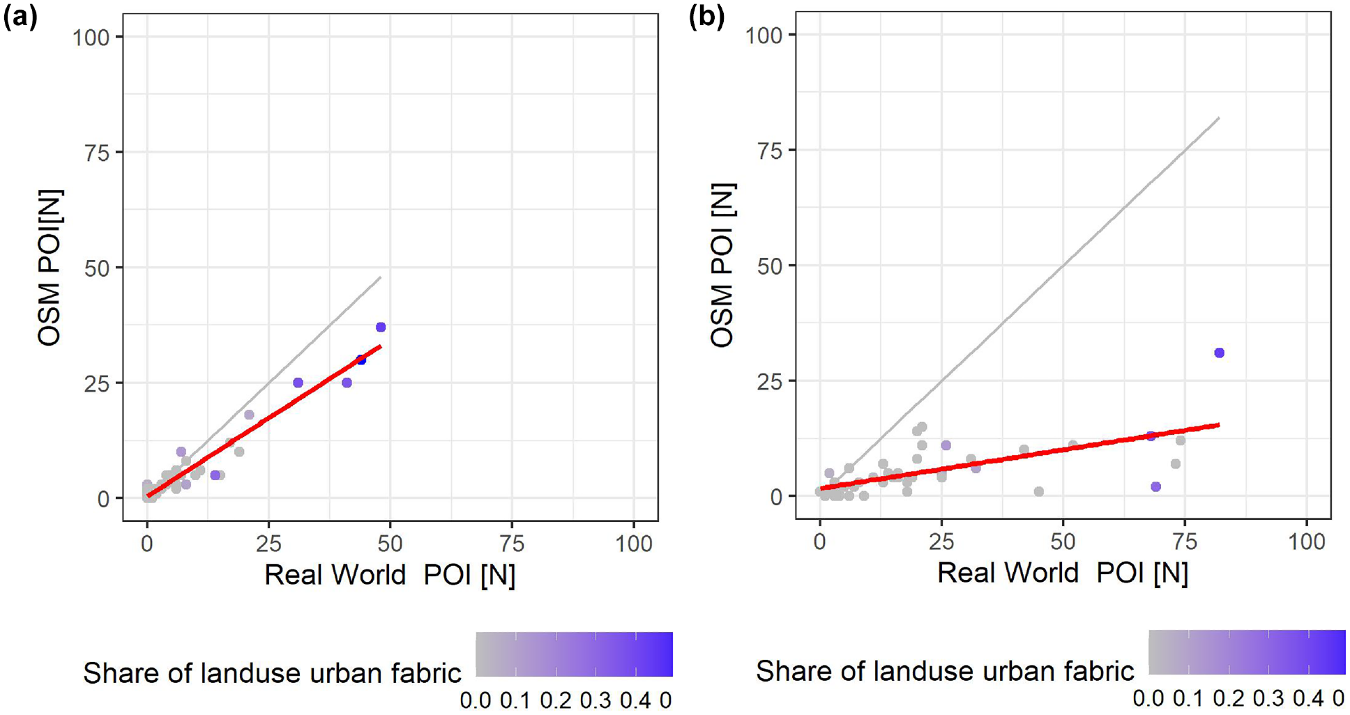
Correlation between points of interest (POI) in OpenStreetMap (OSM) and POI in real-world: (a) shopping and (b) private business.
Therefore, Figure 2 also shows the share of urban areas in the respective survey area. It shows that most of the dense urban areas include a higher number of real-world POI. Nevertheless, explaining the dispersion based on the land use urban fabric alone does not seem to be sufficient.
In a further step, the dependence of the deviation on the real number of POI was examined (Figure 3). It can be seen that, for both activities, the more POI there were in reality, the more POI were missing. In this case, the correlation was more pronounced for private business, which is evident from the higher slope of the compensation line. The graph also shows the relative deviation based on the coloring. It is noticeable that the largest differences tend to lead to smaller relative deviations.
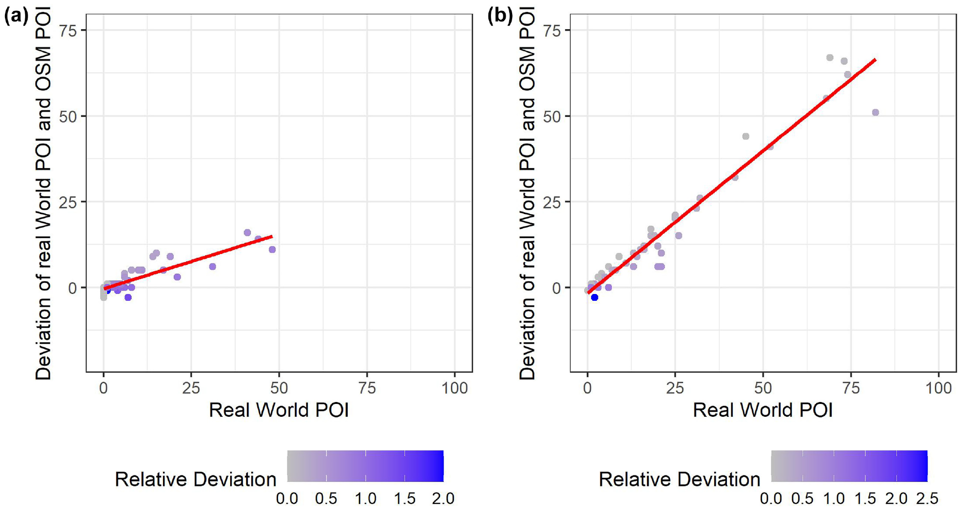
Correlation between deviation and the number of points of interest (POI) in OpenStreetMap (OSM) for (a) shopping and (b) private business.
We also graphically evaluated the saturation indicator in the form of Figure 4. A comparison is made with the relative deviation that could be observed in reality, since the saturation factor also tries to reflect this relationship. The bisector is shown in gray, on which all points would lie if the indicator had perfect significance. Because of the lack of a minimum number of OSM elements, no saturation curve could be estimated for some areas. For these areas, the saturation indicator is 0. In the graphical evaluation, there is hardly any correlation between the relative deviation and the indicator. This is true for both activities and also for all buffer sizes examined. Consequently, this intrinsic indicator alone is not sufficient to explain the dispersion of deviations. In the following, the interaction of different indicators will be examined.
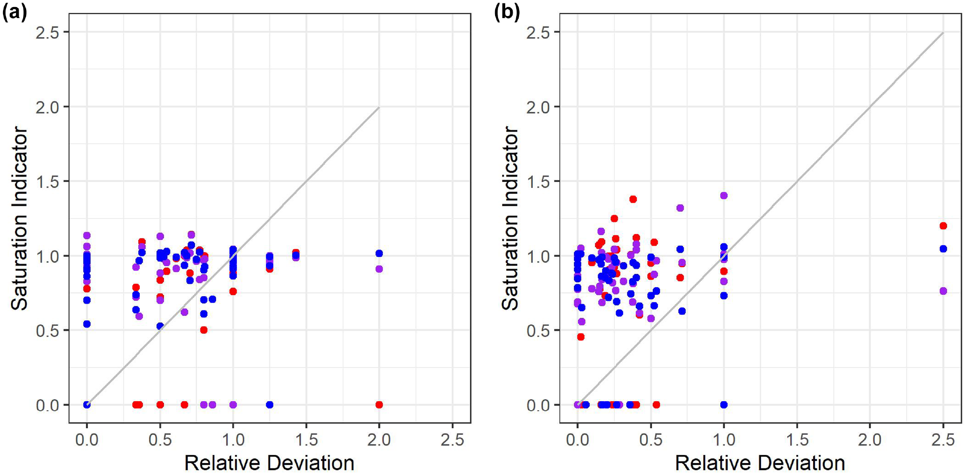
Correlation between relative deviation and estimated saturation for the surveyed areas, a 1 km buffer, and a 2.5 km buffer for (a) shopping and (b) private business.
Model Estimation
To explore dependencies between the features described above and the absolute and relative deviation of OSM POI from real-world POI, we used regression models. Since the number of data points was rather small and we only performed an analysis and no prediction, we did not split into test and training data. Therefore, we expect the model to be overfitted and, consequently, rather focus on qualitative model analyses. For the model analysis, we used the pycaret package for python with all its related packages ( 27 ).
We processed the data to be suitable for regression models. First, we created dummy variables for categorical variables. Second, we checked the data for multicollinearity and applied the built-in function of pycaret to drop one of two identified features using a threshold of 0.8. Third, we dropped features with low variance, which met both of the following conditions: either the count of unique values in a feature divided by the sample size is smaller than 10% or the count of the most common value divided by the count of the second most common value is larger than 20.
We first derived the most suitable model type testing several model types (e.g., random forest, extreme gradient boosting, naive Bayes) on our data and compared the model scores (e.g.,
The quantitative metrics for model performance for the AdaBoost regression models for the activities shopping and private business show a good fit. The
Model-Based Analysis
Since AdaBoost models do not provide interpretative parameters in the way that parametric regression models do, we need to use other measures to gain insights into the data. Two popular measures are variable importance measures (VIM) and partial or feature dependence plots. As measure for both analyses, we used the Shapley additive explanations (SHAP) values ( 30 ). SHAP values attribute the average feature contribution with respect to the prediction of the response. The SHAP value can take positive (positive contribution) and negative (negative contribution) values. Since VIM usually only show the overall importance of the independent variable for the prediction of the dependent variable, we used the absolute SHAP values. For the feature dependence plots, to further analyze the data and gain more insights, we used the regular SHAP values with signs. However, these measures are only capable of providing qualitative insights (e.g., positive or negative influence). Since the size of the data set is rather small, quantitative analyses would be limited anyway.
The choice of the dependent variable is crucial for the explanatory power of the model. To derive a suitable dependent variable for model analysis, the following aspects have to be taken into account. The absolute deviation between OSM POI and real-world POI depends on the number of real-world POI—a larger total number of real-world POI increases the likelihood of missing POI in OSM. Further, the importance of the measured difference between OSM POI and real-world POI decreases significantly as the number of POI increases (see Figure 3). In that case, the ratio between OSM POI and real-world POI is a more suitable dependent variable. Nevertheless, when the number of observations is small, the use of a ratio is problematic because of a high influence of random interference. Additionally, the optimal ratio between OSM POI and real-world POI of unity can lead to problems in the interpretation of the model results. For ratios larger than unity, a decrease in the SHAP value indicates a positive influence, whereas it is the opposite case for ratios smaller than unity. Therefore, without looking at single data points, it would be almost impossible to interpret a positive or negative SHAP value in the feature dependence plots.
Consequently, two main requirements arise that the dependent variable should satisfy. First, it should account for the absolute deviation depending on the total number of real-world POI, which leads to a relative value. Second, since we need to use a relative value, the best case is a ratio of 1. Therefore, cases of a ratio larger or smaller than 1 should be handled equally. These requirements lead to the calculation of a new dependent variable v (as shown in Equation 5) to measure the completeness of OSM POI. While the difference between real-world POI and OSM POI describes the completeness of the OSM database, the ratio of completeness to real-world POI allows us to handle different amounts of POI measured. Moreover, the absolute of the ratio allows the model to treat negative and positive deviations equally.

Variable Importance Measures (VIM)
Figure 5 shows the VIM for the activities shopping and private business. The SHAP value was used as the measure of variable importance. Whereas intrinsic OSM features (saturation index, POI density) and demographic features were the most important features for the completeness of shopping POI, land use features were the most important features for the completeness of private business POI. The important land use categories for the completeness of shopping POI described mainly urban context, whereas for the completeness of private business POI, urban (urban fabric, green urban areas), and non-urban context (other) were ranked high in the VIM. Taking into account that in data processing, strong multicollinearity was eliminated, one can assume that the various spatial resolutions were not strongly correlated and could therefore be combined in one model, although only focusing on one spatial resolution in model analysis is insufficient. This theory is also supported because the features showed no preference for a specific area size. Some features were even important for different area sizes. Consequently, in the further analysis, we focus on the features themselves rather than on the area size they are calculated for.
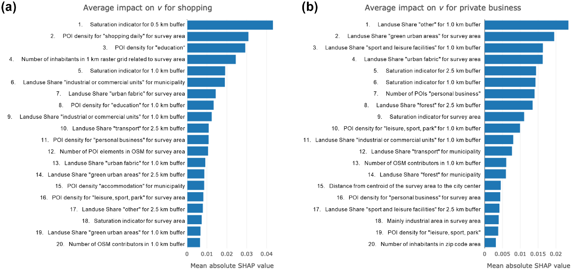
Variable importance measures (20 highest) of the adaptive boosting (AdaBoost) models for (a) shopping and (b) private business.
Land Use
Figure 6 shows the feature dependencies for the shares of the land use features urban fabric in the survey areas and sport and leisure facilities in the 1.0 km buffers, as well as the density of the corresponding POI densities in the survey areas. Whereas the POI density increases for both activity types with the share of the urban fabric areas, this is not the case for the land use areas for sport and leisure facilities.
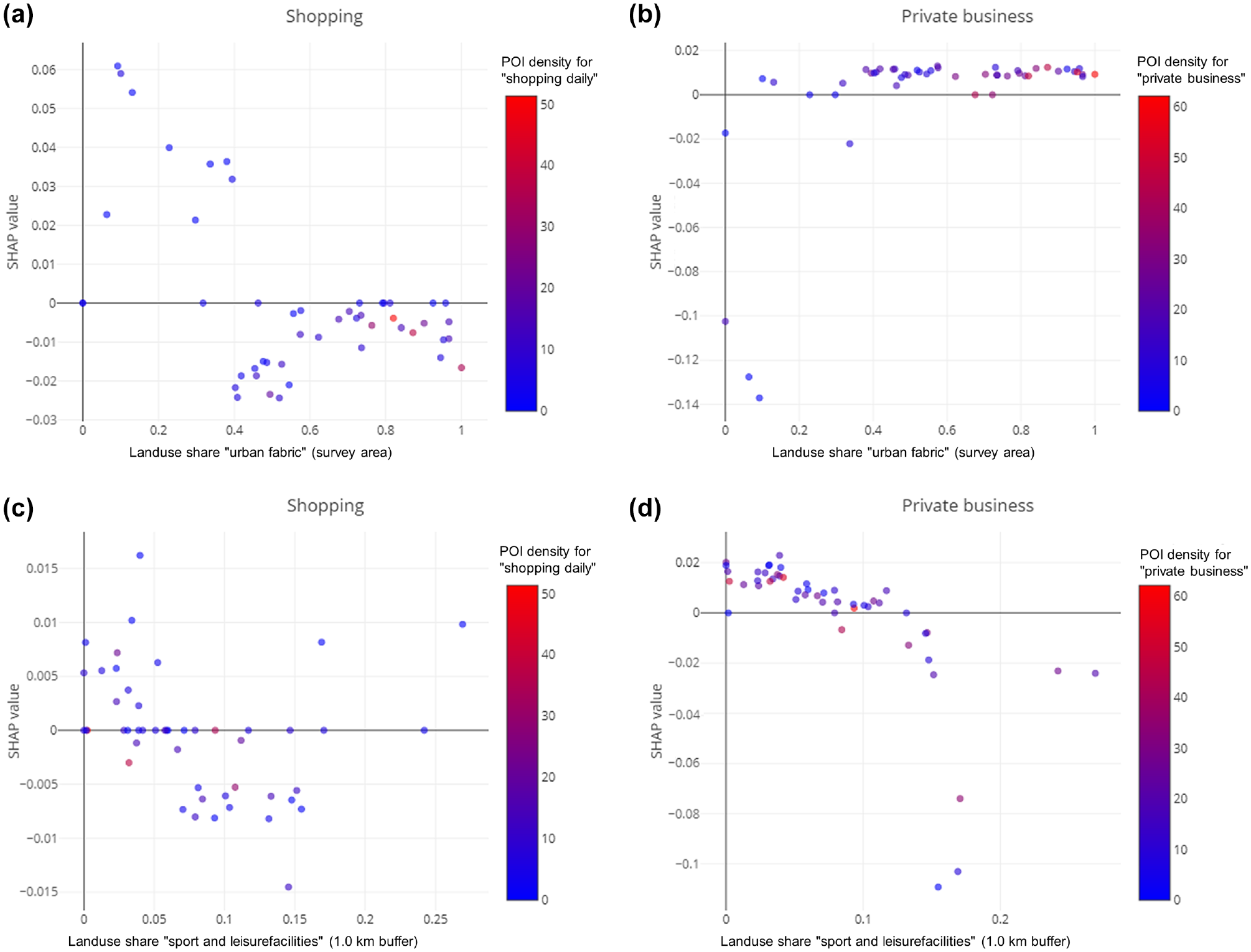
Feature dependence plots for land use features urban fabric and sport and leisure facilities for shopping (a, c) and private business (b, d).
This indicates that sport and leisure facilities can be located both in dense and less dense built environments. The feature dependence for the respective land use shares shows that the completeness of shopping POI is influenced by the urban density, which is not the case for private business POI. A larger share of urban fabric areas as well as higher POI densities rather indicates a worse completeness of private business POI. This could be because many facilities for the activity private business can hardly be recognized on passing by, which is important for being considered in OSM, as previous work indicated ( 12 ). Looking at both land use and POI density the results indicate that hidden private business POI occur more often in dense urban environments. However, higher land use shares for sport and leisure facilities indicate a higher completeness for both activities, since they are usually large attractors and therefore might also attract other POI to settle around.
Historical OSM Data
Figure 7 shows the feature dependencies for the intrinsic OSM features based on the saturation indicator and the number of persons who have contributed to OSM in the survey area so far based on historical data. The indicators on which the analyzed features are based on have not been evaluated with real-world data yet, so this is the first time their explanatory power can be analyzed using extrinsic data. As already seen in the VIM, the saturation indicator has an important influence on the completeness.
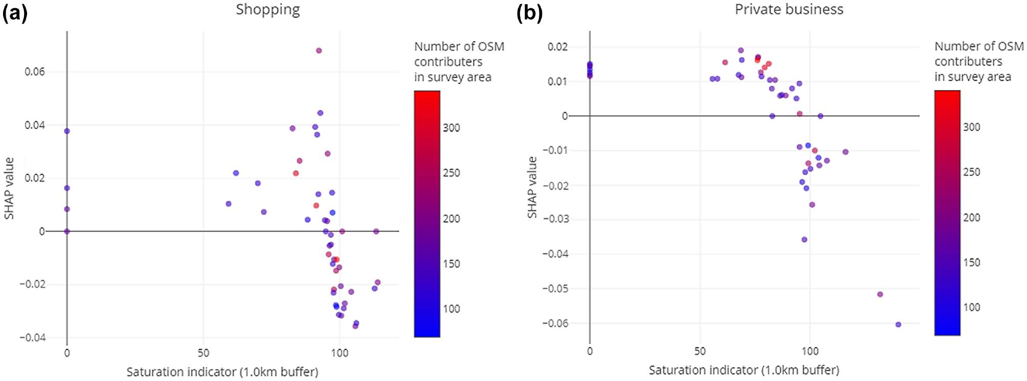
Feature dependence plots for intrinsic OpenStreetMap (OSM) features based on the saturation index and number of OSM contributors for (a) shopping and (b) private business.
The feature dependence plots show that the influence is as expected for both activities: for a saturation lower than 100%, the influence on the deviation of the number of POI is positive, resulting in lower completeness. Around 100% saturation rate, the influence turns into negative figures, indicating a higher completeness. Further, the plots show that the saturation indicator is not correlated linear with the number of contributors and therefore has no effect on this dependency.
Current OSM Data
Figure 8 shows the feature dependencies for the intrinsic OSM features based on the density of OSM POI and the distance from the centroid if the survey area to the city center is based on current data. It can be seen that higher POI densities also have a positive influence on the completeness. However, this effect is more distinct for shopping than for private business. For shopping, lower densities might also correlate with the distance to the city center, whereas this effect is also not as strong for private business. Further, shows that the effect does not increase linearly with the POI density, but is approaching an asymptote and is more or less constant for densities above 10.
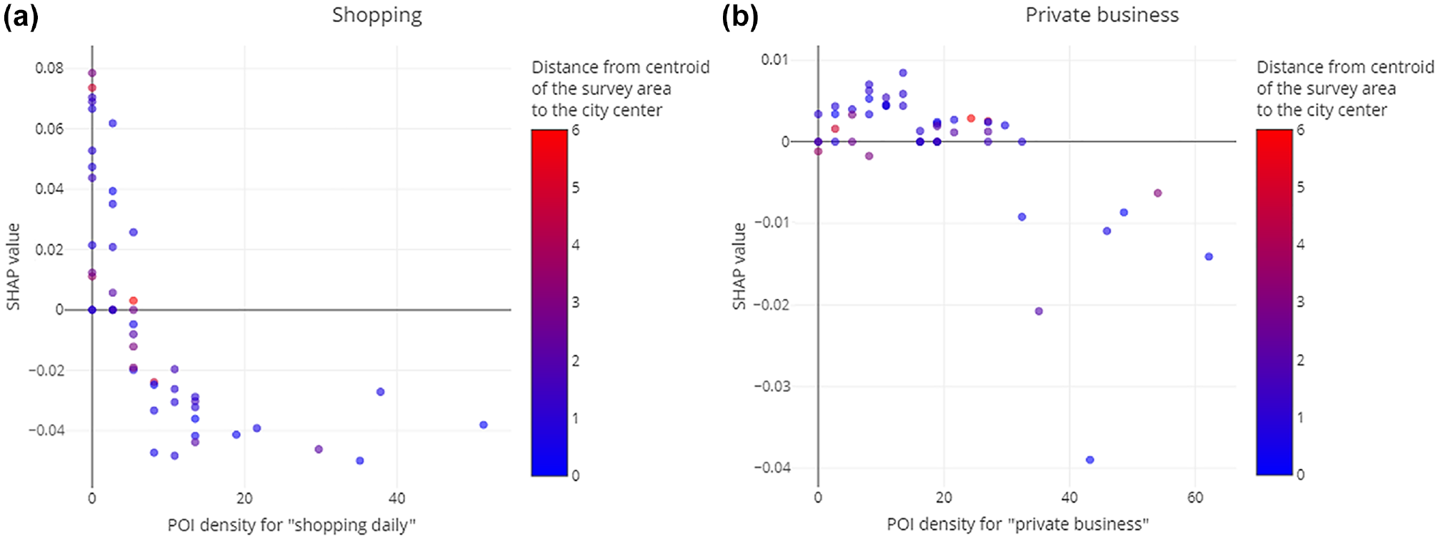
Feature dependence plots for intrinsic OpenStreetMap (OSM) features based on the number and densities of points of interest (POI) for (a) shopping and (b) private business.
Socio-Demographics
Figure 9 shows the feature dependencies for the demographic indicators based on the number of inhabitants. For both activities, different spatial aggregations for the indicators were chosen because of the screening for multicollinearity in data preprocessing. We found that with an increasing number of inhabitants the completeness was influenced positively on different spatial aggregation levels. For both activities, the number of inhabitants might also correlate with POI density. However, the effect was larger for shopping as for POI densities. Furthermore, the influence of the number of inhabitants on completeness was also not linear and seemed to approach an asymptote for more than 5,000 inhabitants per square kilometer for the 1.0 km raster grid and 20,000 inhabitants for the zip code areas.
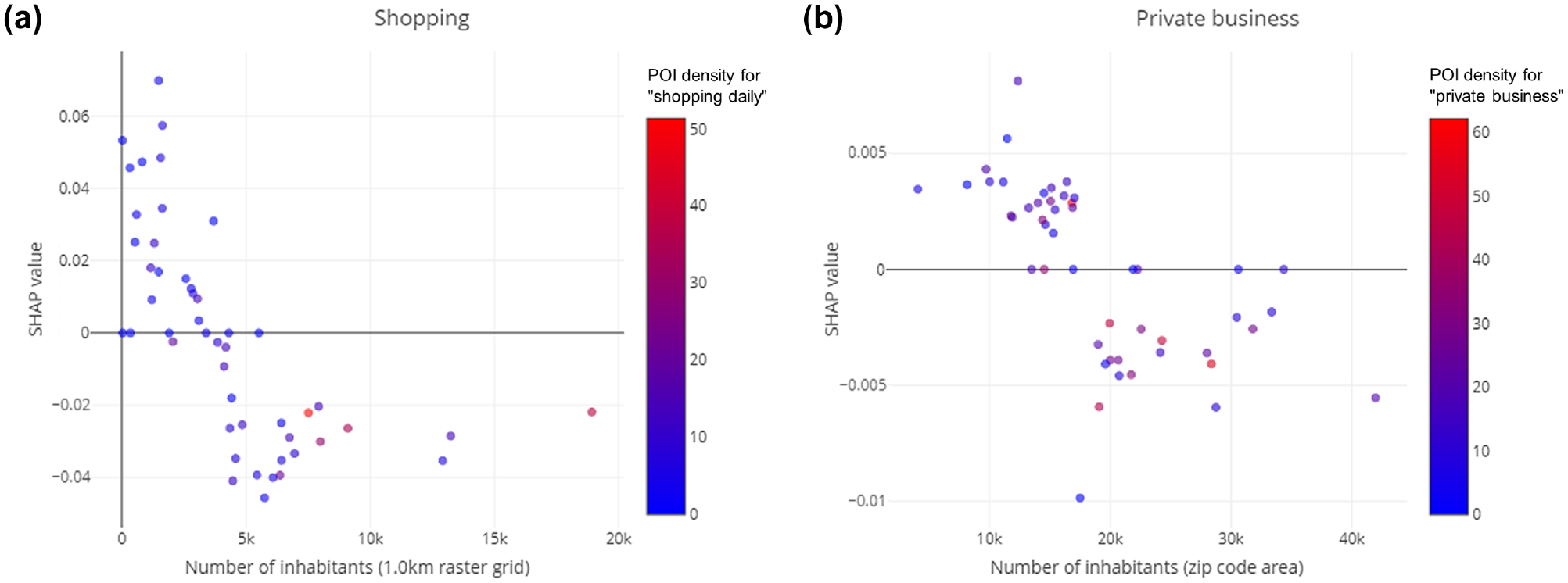
Feature dependence plots for demographic features based on the number of inhabitants for (a) shopping and (b) private business.
Conclusion
In this work, we assessed the quality of POI data from OSM. We compared POI from OSM with large-scale real-world data surveyed in 49 areas. These areas are spread all over Germany and mostly represent urban and suburban areas. The quality assessment was optimized for the use as demand and supply data for travel demand models. Therefore, we categorized the POI of common activities used in travel demand models and chose the activities shopping and private business as example categories for this work.
We found that, for both categories, the POI are not completely mapped in OSM. The deviation of OSM POI and real-world POI is higher for private business POI, though. This could be because shops have to attract customers and therefore have a higher visibility (e.g., signs or display windows), whereas private business POI (e.g., doctors, small agencies, small craft businesses) often lack visibility. This finding is in line with our findings from previous work ( 12 ).
We also found for both activities that more dense urban areas imply a higher completeness of OSM POI, although this effect is stronger for shopping POI. We therefore can also confirm previous findings from the literature ( 1 , 8 , 9 ).
We further found that intrinsic indicators, such as the saturation index, constitute a good measure to assess the broad level of completeness. Since surveying real-world data is very cumbersome, this finding reinforces intrinsic measures and supports that further research is important to improve intrinsic quality measures to assess the quality of OSM data.
However, our work is only based on the data of 49 survey sites. Therefore, although the locations are spread all over Germany, the models are expected the be overfitted on the data from the survey sites. Transferring the results to whole of Germany, or even Europe or the rest of the world, should therefore be done with care. However, with our results being in line with previous findings, we argue that more general findings can be transferred quite well.
Consequently, for our future work, we will collect more data by locating additional real-world POI in up to 50 other survey areas, also focusing on more rural areas. Additional data might allow splitting up the data in training and validation data and, therefore, allow to train a model which is able to predict the completeness of OSM POI. This is important because, for the use in travel demand models, not only the knowledge about incomplete POI is relevant, but also the amount of the deviation to be able to weight the OSM data to derive realistic input data.
Footnotes
Author Contributions
The authors confirm contribution to the paper as follows: study conception and design: C. Klinkhardt, F. Kühnel, M. Heilig, S. Lautenbach, T. Wörle, P. Vortisch, T. Kuhnimhof; data collection: C. Klinkhardt, F. Kühnel, M. Heilig, S. Lautenbach, T. Wörle; analysis and interpretation of results: C. Klinkhardt, T. Wörle, F. Kühnel, M. Heilig, S. Lautenbach; draft manuscript preparation: T. Wörle. All authors reviewed the results and approved the final version of the manuscript.
Declaration of Conflicting Interests
The author(s) declared no potential conflicts of interest with respect to the research, authorship, and/or publication of this article.
Funding
The author(s) disclosed receipt of the following financial support for the research, authorship, and/or publication of this article: The survey was conducted in the project Cities in Charge (reference no. 01 MZ 18005C), funded by the German Federal Ministry for Economic Affairs and Climate Action. Sven Lautenbach acknowledge funding by the Klaus-Tschira Stiftung. We also would like to thank all OSM contributors.