Sage Journals: Discover world-class research

Abstract

Travel demand models benefit from integrating social networks to capture socially induced travel behavior, such as destination choice. One of the obstacles to this integration is the lack of reliable and realistic social networks as input. This paper introduces an agent-based method to synthesize social networks with global characteristics and heterogeneous ego-centric homophilies (distance, age, gender) for a substantial population (approximately $10^{6}$ individuals). Drawing on data from an ego-centric snowball sample, it successfully replicates age, gender, and distance homophilies while achieving significant social network-level transitivity and clique structures. The study uses epidemic spread as a case study to explore the effects of incorporating social networks and coordinated destination choices into travel forecasting. Results show that while the total number of infections remains unchanged, the integration of social networks and coordinated destination choices affects contextual aspects of infection events. Coordinated travel through social networks accelerates the initial spread and affects the spatial distribution of epidemics. The findings underscore the importance of integrating social networks and joint travel to more accurately represent social travel behavior.

Keywords

planning and analysis transportation demand forecasting choice models demand estimation forecasts/forecasting models/modeling trip generation modeling

Human mobility, like many other aspects of human behavior, is socially driven. In recent years, the transportation modeling field has increasingly tried to capture the obvious link between social connections and travel behavior ( 1 ). Various elements of travel behavior, including the creation of travel activities, choice of destination, and mode of transportation, and, by extension, travel demand modeling, are affected by social connections ( 1 ). No model, however, has yet integrated and implemented a social network in a complete travel demand model framework.

As we identify this gap and move to implement models that more actively consider social connections, it becomes crucial to have representative models of underlying social networks. Real-world social networks, however, are notoriously difficult both to quantify and replicate. A series of publications originating from ETH Zurich, highlighted by Kowald and Axhausen ( 2 ), Arentze et al. ( 3 ), and Dubernet ( 4 ), have contributed significantly to both the data collection and synthetic social network generation sides of this problem, particularly through the collection and analysis of their ego-centric, snowball survey dataset. Ego-centric here means a network consisting of an ego or focus point, connected to alters, for example, family members, co-workers, and so forth. Their research has identified the importance of socio-demographic homophilies and geographic distance as key ego-based characteristics of such social networks, while literature on social networks more generally provides expectations about network-level characteristics, like transitivity and clique structure. While the literature abounds with examples of synthetic general network and social network generation, it remains difficult to find methodologies that successfully unify these two perspectives.

Recently, the application of travel modeling to epidemic spread has emphasized the importance of integrating social networks within such a framework. Person-to-person contact is crucial to epidemic spread models. Since social networks can strongly influence travel behavior and contact patterns, it is beneficial to add in social networks when using travel demand models to simulate disease spread. Previous researchers have used agent-based epidemic models to better understand and predict the spread of infectious diseases in Singapore ( 5 , 6 ), the Twin Cities (Minneapolis–Saint Paul, MN) ( 7 , 8 ), or Berlin ( 9 ). Similarly to the gap in more general travel demand modeling, none of these studies has explicitly considered the impact of social networks on epidemic spread.

Thus, this research endeavors to generate a social network for an existing synthetic population and apply it to a travel demand model. The resulting travel demand is then applied in epidemic modeling using EpiSim, an infection dynamics model developed by Müller et al. ( 9 ) that is coupled with the Multi-Agent Transport Simulation (MATSim, https://github.com/matsim-org/matsim-EpiSim-libs). As a first step, we focus on adding coordinated destination to travel demand generation, and infection rules influenced by social connections in EpiSim to see the impact of social network on infection spread patterns and rates.

The rest of this paper is largely structured following this pipeline from social network synthesis to epidemic modeling. The Literature Review section discusses significant literature associated with social networks, the current state of joint travel modeling, and epidemic modeling. The Methodology section outlines the algorithm for the generation of the synthetic social network and the adaptations to the travel demand model that account for coordinated destination travel. In the Results section, we discuss the quality of the generated synthetic network and the impact of coordinated destination on the travel model and the recorded infections.

Literature Review

We explore the current state of the art in social network generation, with a focus on its development within the transportation field. In conjunction, we discuss the modeling of social activity participation and travel. Lastly, we briefly contextualize the third component of this study, the epidemic spread model. For our purposes, a social network is defined as a social structure graph composed of nodes and edges, where each node represents a person and each edge represents the presence of a connection between two nodes, or persons.

Social Network Generation

The study and synthesis of social networks is a field unto itself. The structure of real-world social networks, particularly those that could motivate leisure travel, is difficult to capture. In general, the task at hand requires the balancing of social network-level characteristics and ego-centric preferences. That is, we must replicate the more general patterns of social networks—community structures ( 10 , 11 ) and higher transitivity ( 12 , 13 )—while also capturing agent-based homophily preferences, that is, the tendency of people to associate with others who possess similar characteristics ( 14 ). Successfully capturing either of these aspects is a computationally difficult task, particularly at the desired scale. Finding proper data to match is also difficult, as, while there are various complete and highly connected social networks publicly available for study ( 15 ), these social networks are generally embedded in online environments and they thus lack characteristics that may influence social and leisure travel decisions. Among other flaws, this online embedding mitigates the impact of geographic distance, which is of significant concern and is explored in depth in Arentze et al. ( 3 ), Mok and Wellman ( 16 ), and Illenberger et al. ( 17 ).

A notable dataset that provides this type of geographically-embedded and demographically informed connection data comes out of research at ETH Zurich. Kowald and Axhausen ( 2 ) performed a multi-year snowball survey that provides a key source for this topic. The resulting dataset yields a total of $793$ egos and $14, 326$ unique names. While the demographic data is extensive, snowball sampling, by nature, leads to many branches connected only to a single ego. Therefore, any analysis of this data must focus on ego-centric metrics, not global network characteristics. Informed by this dataset, previous work has established that age, gender, and geographical distance homophilies are the most significant demographic attributes in social networks that affect leisure travel ( 3 , 4 , 17 ).

More complete social networks, such as the Facebook social networks studied by Mayer and Puller ( 12 ), can provide insight on metrics like transitivity and community structure. These social networks often exhibit so-called “small-world” characteristics, as initially discussed by Watts and Strogatz ( 18 ).

The classical approach to synthesizing such social networks is through a class of models known as exponential random graph models (ERGMs). These models account for homophily and social network structure by calculating probabilities for the existence of edges based on node homophily and then adjusting the probability of a connection to account for local social network structures, for example, increasing the likelihood of a connection if two nodes already share a mutual neighbor ( 19 ). These models are, however, notoriously difficult to tune and do not necessarily scale to the sizes necessary. Recently, as detailed in Snijders et al. ( 20 ), stochastic actor-based models have emerged as another attempt to use ego-centric properties and agent-based, local formation mechanisms to more accurately represent agent preferences while pursuing some type of social network structure. These models are particularly useful for considering the dynamic evolution of social networks.

Within the context of leisure travel social networks and based largely on ETH Zurich’s snowball data, Illenberger et al. ( 17 ) pursue an ERGM for roughly 40,000 nodes, successfully accounting for homophily, though falling short in social network structure, particularly transitivity. Arentze et al. ( 3 ) explicitly account for transitivity via a link probability model, but do so for just 3,301 agents. Work by Dubernet ( 4 ) generates a social network with a heuristic that accounts for socio-demographic and geographic homophily in addition to clique distribution, but does not account for agent-specific preferences.

A notable tool for embedding highly transitive social network structures in an otherwise homophily-based model is the concept of triadic closure. Triadic closure is the principle that, among a group of three agents, $A$ , $B$ and $C$ , if there are connections $A - B$ and $A - C$ , there is an increased likelihood of connection between B and C. This concept was first explored by Granovetter ( 21 ) and is used to augment a homophily-based model in Asikainen et al. ( 13 ).

In general, mathematical social network synthesis methods are difficult to tune for both ego-centric and social network-level attributes, particularly given the need to realistically embed these connections geographically. Moreover, social friendship connections that inspire travel, which incurs costs of both time and distance, are significantly different from low-cost, online connections, making it difficult to apply standards from many prominent datasets to fill out the social network structure suggested by snowball data.

Finally, homophily models tend to treat homophilies as constant across demographic groups ( 3 , 4 ). While computationally simpler, this is not necessarily true within the mentioned snowball data, as will be shown in the Determining Social Network Formation subsection of the Methodology section. This suggests that there is room for an agent-based approach that accounts more carefully for demographic differences during formation while also employing stochastic techniques, like triadic closure, to achieve a social network with small-world characteristics ( 13 , 18 ).

Social Travel Modeling

There have been a few studies that attempted to integrate formed social networks into transport simulation frameworks. Van den Berg et al. ( 22 ) and Moore et al. ( 23 ) studied destination sharing among socially connected people. Arentze and Timmermans ( 24 ) looked at joint activity generation and participation between multiple persons, taking into account the information exchange and preferences of multiple persons. However, this was confined to persons of the same household. Ettema et al. ( 25 ) followed up, generating an inter-household social network for use in a Land Use and Transport Interaction model influencing long-term residential location decisions. Han et al. ( 26 ) furthered the study by incorporating this generated social network in the FEATHERS agent-based framework. Hackney and Marchal ( 27 ) developed a social network module for MATSim as an exploratory exercise testing how social networks lead to collaborative activity scheduling through which social interactions act as information exchange. Marchal and Nagel ( 28 ) conducted a case study on how discretionary activity destination choice was influenced by information exchange via a social network created using “spatial reinforcement à la pheromones in ant colonies.” This series of studies considered a generated social network in the framework in the context of social influences on household or individual agent decisions, but did not explicitly incorporate joint decision-making as influenced by social networks. In addition, Ronald et al. ( 29 ), Ma et al. ( 30 ), and Dubernet and Axhausen ( 31 ) presented an agent-based system that integrates joint decision-making mechanisms based on rule-based simulations of a bargaining process.

However, these studies either lack a realistic and representative social network, or are conceptual experiments instead of actual integration and implementation of a social network in a complete travel demand model framework.

Epidemic Spread Model

In recent research on agent-based epidemic models, epidemic transition models varied from the simplest Susceptible-Infected model (SI), in which agents are exposed only while traveling ( 8 ), to the more complex Susceptible-Exposed-Infections-Removed (SEIR) model with exposure while traveling and at destinations ( 6 , 9 ). On the other hand, travel demand generation in these models was rather simplistic, as it replicated transit trips ( 7 , 8 ) or smart-card bus trips ( 5 , 6 ). A notable exception is Müller et al. ( 9 ), who replicated activity-based trajectories from mobile phone data and used traffic and transit assignment in MATSim. Müller et al. ( 9 ) at the Technical University of Berlin developed the model known as EpiSim, an infection dynamics model on top of a person’s movement trajectories. Furthermore, Müller et al. ( 9 ) validated the results of EpiSim with COVID-19 hospital cases in Berlin. It allows testing of intervention policies such as home-office mandates, mask-wearing mandates, and so forth. Since it is open source and readily coupled with MATSim, EpiSim presents an inviting option for studying the effects of social network in a travel forecast model.

EpiSim comprises several models: the contact model, infection model, and disease progression model ( 9 ). The contact model defines who comes into contact with whom. Persons at the same location or facility can come into contact with and infect each other. These facilities could either be in transit or at an activity location such as home or work. When two persons come into contact, a probability of infection is calculated using the infection model, which gives this probability based on contact intensity, contact duration, viral shedding, and intake. If a person becomes infected, the disease progression model then gives the probability that this newly exposed and infected person progresses to the next stage of the disease. The exposed person can become infectious, recover, or get worse. The simulation runs for a year or until no more infections occur. For more details on EpiSim, please refer to Müller et al. ( 9 ).

This review is by no means exhaustive on each of the three stages of this research. Still, it suggests both the successes and gaps in the individual fields, and provides perspective on how considering the pipeline as a whole motivates and synergizes with the specific methodologies we propose in the following section.

Methodology

The methodology employed creates a social network on top of an existing synthetic population. As a case study, the social network is then applied to a travel demand model with tailored joint travel and an epidemic model; Figure 1 shows the model framework. Our study area is the Munich metropolitan region, including the City of Munich and the surrounding cities of Augsburg, Ingolstadt, Landshut, and Rosenheim. This area has a population of 4.5 million in roughly 2.1 million households.

Figure 1.

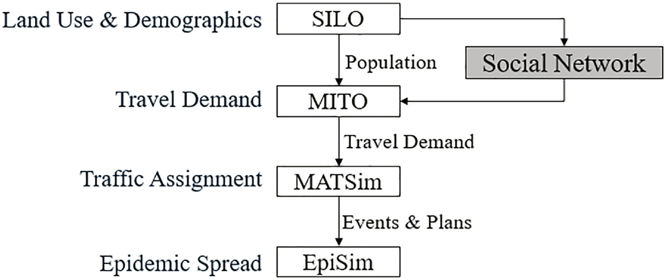
Modeling framework including social network.

Briefly, we use a 5% sample of a synthetic population from the Simple Land-Use Orchestrator (SILO) ( 32 ) to generate a geolocation-based social network for the Munich area. This population and network is then passed to the open source agent-based Microscopic Transportation Orchestrator (MITO) ( 33 ), which simulates travel demand for each agent. Depending on the scenario, this includes updated rules for paired or clique-based coordinated destination travel. This demand is assigned to road and transit networks using MATSim ( 34 ). Finally, EpiSim runs the epidemic simulator on MATSim’s one-day trip profile for an entire year.

Determining Social Network Formation Attributes

To enter the social network generation stage, we require a synthetic population for the region, which we take from the SILO land-use model. SILO generates a synthetic population based on census data and iterative proportional updating ( 32 ). SILO synthesizes both individual and household level characteristics for all residents of the greater Munich metropolitan area, including household composition, location, and education or work locations. Therefore, a level of social connection is already implicit through shared households, work places, and education places. However, there are no additional social or friendship connections. Therefore, we focused on generating a friendship network on top of an existing household and work/education network.

The goal is to generate this friendship social network for a 5% sample of this synthetic population. There is a lack of data at the extremes of the age ranges, so we do not consider the agents under the age of 10 and will consider anyone over the age of 80 functionally to be 80. Aligning with previous work in the travel behavior space, homophily is the key mechanism by which agents are connected. The three key agent-level attributes against which we match are distance, age, and gender (2–4, 17 ). While it could be fruitful to extend to other attributes—income, education level, religious affiliation, for example—the addition of any attribute during formation significantly increases computational complexity and runtime. It is possible that, in the future, by vectorizing attributes and performing an aggregated characteristic similarity calculation, we may be able to expand the number of attributes that are possible to model, though that is not the goal of this iteration.

Taking inspiration from stochastic actor-based models ( 20 ), Dubernet’s ( 4 ) clique-focused model, and Asikainen et al.’s ( 13 ) triadic closure approach, the proposed formation algorithm uses specific search strategies to maximize homophily matchings while producing a reasonable network structure, including some measure of clique formation, in a reasonable computation time.

To do so, we stochastically assign to each member of the population—referred to as either agents or egos—attributes from distributions defined by the snowball dataset ( 2 ). We proceed with the assumption that the Munich study area bears sufficient resemblance to the adjacent Swiss population surveyed in the snowball dataset and thus we can apply derived homophily and other attributes to our study area. In particular, each agent draws its desired degree and baseline age and gender homophily preferences according to its own demographic characteristics. Degree here refers to the number of social connections an agent has, represented in the network as number of edges connected to a node.

This approach, which introduces “heterogeneity in homophily,” is a departure from the methodologies in Arentze et al. ( 3 ) and Dubernet ( 4 ), where all agents draw from the same distributions for these characteristics. 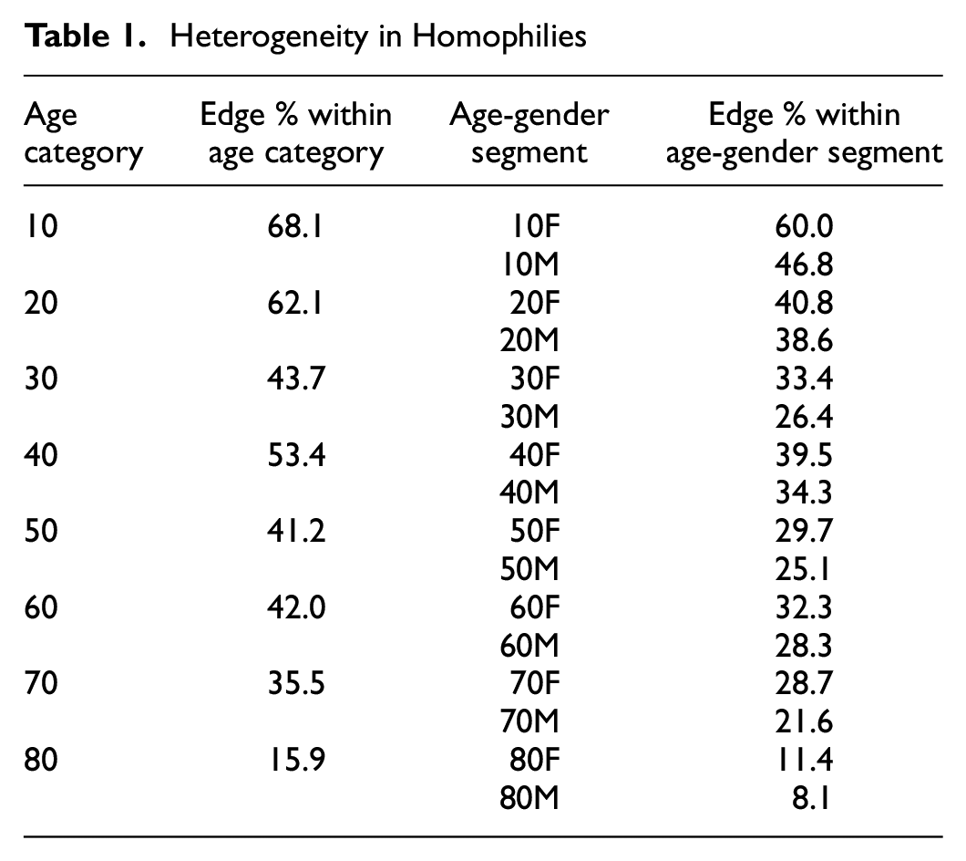To introduce a mechanism for this heterogeneity in homophily, while preserving computational tractability and reasonable data segmentation, we divide the data into 16 segments by binning the $793$ snowball egos into eight 10-year age brackets and the two response genders. In Table 1, we illustrate the significance of this heterogeneity through the percentage of edges formed within age brackets and within age-gender segments. This result aligns with the intuition that a 10-year age gap is perceived differently between agents who are 15 and 25 than it is among agents who are 65 and 75. Similarly, as shown in Figure 2, there are significant differences in the degree distributions across segments.

Table 1.

Heterogeneity in Homophilies

Age category	Edge % within age category	Age-gender segment	Edge % within age-gender segment
10	68.1	10F	60.0
10		10M	46.8
20	62.1	20F	40.8
20		20M	38.6
30	43.7	30F	33.4
30		30M	26.4
40	53.4	40F	39.5
40		40M	34.3
50	41.2	50F	29.7
50		50M	25.1
60	42.0	60F	32.3
60		60M	28.3
70	35.5	70F	28.7
70		70M	21.6
80	15.9	80F	11.4
80		80M	8.1

Figure 2.

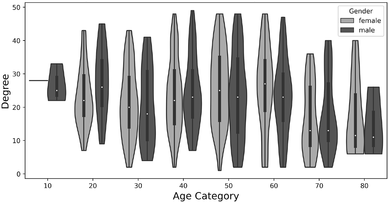
Heterogeneity in degree distribution based on age and gender. Gaussian kernel density estimators are used downstream to smooth data for eventual model input.

With this in mind, we generate a smoothed distribution for agent degrees by segment and a discrete distribution mapping the proportion of edges from each segment to all 16 segments (eight age brackets × two genders). Each member of the synthetic population then draws from the degree distribution of the appropriate segment to gain a “target” degree and is assigned the appropriate homophily distribution, which will be drawn from repeatedly during formation.

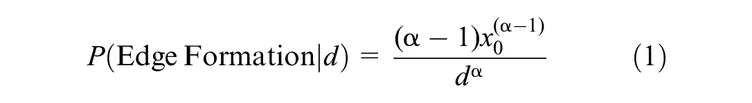
Following Illenberger et al. ( 17 ), we address geographical distance between socially connected agents through a single, “scale-free” power law probability distribution for all edges. Working with a similar dataset, Illenberger et al. ( 17 ) determine that the probability of forming a connection of distance $d$ between any two agents is described by the following distribution function:

P (Edge Formation | d) = \frac{(α - 1) x_{0}^{(α - 1)}}{d^{α}}

(1)

We specify the exponential and scale factor parameters, $α$ and $x_{0}$ , by a least-squares estimation on the distribution of distances between friends in the snowball data that would fit inside the Munich study area. An additional normalizing factor is introduced in the code to ensure that the cumulative distribution function converges to one within the study area.

Finally, transitivity is addressed during formation by a heuristic for triadic closure during the formation step. Friendship searches are performed either from the remaining eligible population or are restricted only to “friends-of-friends.” If an edge is formed through the latter search, this automatically closes a triad and forms a clique of at least three; larger cliques are stochastically formed by chance throughout this type of search. During analysis, we restrict the meaning of cliques maximally complete subgraphs of more than two nodes.

Social Network Formation

The formation method broadly follows the iterative three-step process displayed in Figure 3. In short, at the beginning of each iteration, agents draw a friend-goal dictionary based on their segment-to-segment homophily distribution. Then, the algorithm performs a double-blind matching such that each agent is mutually seeking an agent in the other’s segment; this matching either searches the entire population or restricts each agent to their second degree connections. A connection is only formed if the agents pass a stochastic draw based on the geographic distance between them. If a connection forms, agents update their friend-goal dictionary before searching for further connections. After a round of matching, remaining unsatisfied agents redraw their homophily dictionaries, restarting the cycle.

Figure 3.

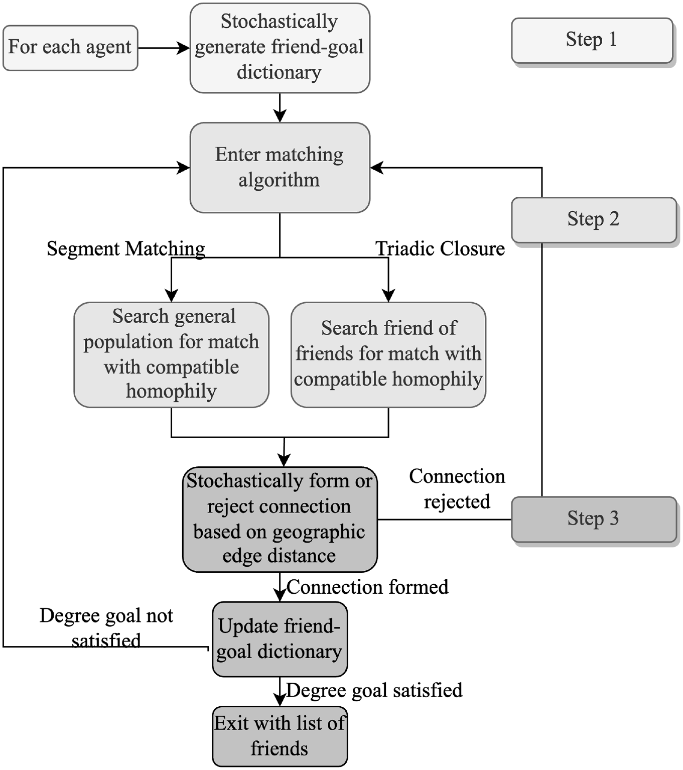
Social network generation steps for each iteration.

In detail, during Step 1 each agent calculates how many degrees, or friends, $k$ , they need to reach their fixed degree goal. Each agent then draws $k$ times from their homophily distribution to form a “friend-goal” dictionary. This determines the segments from which each agent is willing to search for connections during Step 2. Figure 4 illustrates two example agents after an initial draw.

Figure 4.

Sample agents after initial draw.

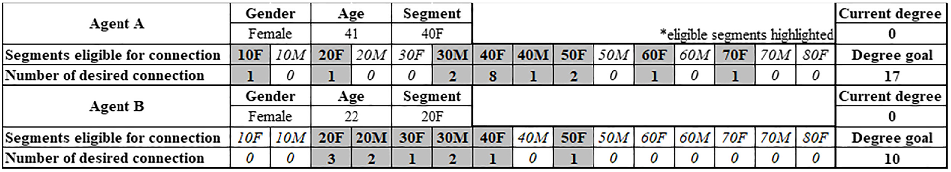
In Step 2, the algorithm matches mutually eligible agents. For example, in Figure 4, Agent A is in the $40 F$ segment and is looking for one connection in the $20 F$ segment; Agent B is in the $20 F$ segment and is looking for a connection in the $40 F$ segment. They are mutually compatible and could be matched.

During Step 2, agents search for matches from the general population or from their second degree connections, that is, friends of their friends. Because this triadic closure heuristic for clique formation is iterative, clique formation does not require any loosening of homophily distributions for formation. The only adjustment to tune for the formation of larger cliques is that second degree connections with whom an agent shares multiple friends are given priority during search.

The algorithm currently forms an initial proportion of agents’ degree goals by matching from the general population. At 25%, it then switches to triadic closure, which reduces the search space but enables clique formation. When progress stagnates, the algorithm switches back to the general population search to complete the remaining connections.

After any potential match is found, this connection enters Step 3 where it is accepted or rejected based on the geographical distance between the two agents. Equation 1 generates a connection probability for this distance, which is then compared with the result of a uniform draw from $(0, 1)$ . If the edge is formed, each agent subtracts one from the appropriate segment of their friend-goal directory. If this completely satisfies either agent’s degree goal, that agent exits the algorithm. Otherwise, each agent returns to Step 2 to search for new connections. After an iteration exhausts its possible matches, all remaining agents stochastically redraw their friend-goal dictionaries via Step 1 and the process repeats.

Because of asymmetries in the homophily matrix and the demographic variation between the snowball and synthetic populations, these stochastic iterations are necessary for everyone to achieve their desired degree. By repeatedly drawing from the segment homophilies, the algorithm induces an equilibrium that balances these asymmetries.

Travel Demand Model and Rule-Based Coordinated Destination

The second part of this study uses an agent-based travel demand modeling suite to generate daily movements of individuals. To achieve this, the synthetic population with the geolocation-based social network was fed into MITO ( 33 ). MITO is an agent-based travel demand model that uses econometric models to estimate trip generation, trip distribution, mode choice, and time of day for each individual in the synthetic population. After that, MATSim ( 34 ) is used as a dynamic traffic assignment model to assign car trips to the road network and simulate public transport trips on the transit system ( 35 ). The individual movements are estimated for a typical 24-h day for the following trip purposes: home-based work (HBW), home-based education (HBE), home-based shopping (HBS), home-based recreation (HBR), home-based other (HBO), non-home-based work (NHBW) and non-home-based other (NHBO).

We extended MITO by adding the rule-based coordinated destination choice. This extension is accomplished by making some modifications to the existing MITO model sequence, as is listed below. After the Trip Distribution step, we add a Destination Coordination step. This step coordinates destination either between two friends or between members of a clique. Compatible trips are defined as trips that have arrival times within 6 h of each other, and are of the same purpose. A Monte Carlo simulation is applied to determine if each pair of compatible trips will be coordinated. We also apply a weighted probability inversely proportional to the geographical distance between the two trips’ original destinations. If compatible trips are determined to be coordinated, we assume the ego is the decision maker, and set the destination and arrival time of the alter’s trip to be the same as the ego’s. After any changes of destination have been made to the trip, the mode choice is run without any modifications. The departure time can then be calculated based on the chosen mode and projected travel time.

The modified MITO model sequence to account for destination coordination is as follows:

Trip Generation

Trip Distribution

Added step: Destination Coordination

(a) For each ego trip, find compatible trips from their alters’ trips

(b) Select a trip from compatible trips based on weighted probability

(d) Additional rules to enable clique travel:

i. Select a random agent’s trips from each clique, find compatible trips from all other members in the clique

ii. Select a trip from each other member in the clique based on weighted probability

iii. Set destination and arrival time of alter trip to be the same as the randomly selected agent’s trip

Mode Choice

Added step: Departure Time Assignment

Epidemic Model Extension

To see the effect of social networks on epidemic spread, we extended the EpiSim model to account for social networks. First, the contact model was modified. This contact model looks at agents when they leave a facility. Under the assumption that people tend to be in greater proximity to those in their social group than they are to strangers, instead of randomly selecting other agents who are at the facility at the same time, we increased the likelihood of being selected if they belong to the same social network. Second, we changed the infection model parameters to consider that persons in the same social network may reduce social distancing, and therefore, the viral load may be increased. This is accomplished by increasing the contact intensity factor. For contacts from within the agent’s social network, the contact intensity is multiplied by a factor of 10. Short of observed data, this factor is an exogenous assumption that ensures a higher infection rate within social networks. The current contact intensities and infection probabilities are set according to those specified in Müller et al. ( 9 ) for the COVID 19 virus.

Scenarios

By varying the addition of social network, coordinated destination choice, and EpiSim disease contact rules, we look at a total of three scenarios. To reduce model runtime, all scenarios use a 5% scaled-down population. The social network is generated after scaling down. EpiSim results are reported after upscaling factors to 100%. .

Base: In the Base scenario, we essentially use the base versions of MITO and EpiSim. The travel demand from MITO does not take social networks into consideration and has no coordinated destination choice. In EpiSim, for an agent at a certain location/facility, a maximum of three contacts are randomly selected from those who are at the same location and the same time as the agent. This number is the base assumed setting in the calibrated EpiSim Berlin scenario ( 9 ). The infection probability is calculated between the agent and each of these three contacts. This is graphically represented in Figure 5, in the left box.

Friends: In the Friends scenario, MITO implements coordinated travel between two agents based on the social network. In this scenario, a maximum of two friends can have their destinations coordinated. In the epidemic model, selection priority is given to those within the agent’s social network. An agent comes into contact with as many contacts as there are in the agent’s social network. The infection probability is calculated for all these contacts. If there are less than three contacts at the location in the agent’s social network, then random agents are selected until there are three contacts. This is seen in the right box in Figure 5.

Cliques: In the Cliques scenario, in addition to coordinated destination between two agents, MITO allows coordinated travel between all agents within a clique. The epidemic model contact rules are the same as in the Friends scenario.

Figure 5.

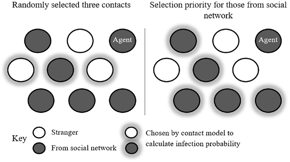
EpiSim contact rules for different scenarios.

Results and Discussion

We now discuss the characteristics of the synthesized social network and the results of the three scenarios to see how the implementation of social network and coordinated destination rules affect the spread of disease.

Social Network Synthesis

The current algorithm is built in Python and makes use of the NetworkX package ( 36 ). The algorithm scales roughly as $O (n^{2})$ and runs in 30 min, generating $1, 786, 880$ edges for $202, 401$ nodes. Removing nodes with zero connections, there are $195, 979$ agents; there are 10 fully connected components: one of $195, 961$ agents and nine dyads of otherwise unconnected agents.

Age and Gender Homophilies

Figure 6 summarizes the ego-centric distribution of age distributions by age category. In general, the synthetic network demonstrates a higher reversion to the mean, suggesting that agents tend to exhibit more significant age-based homophilies. This holds when performing similar calculations on the complete, unweighted edge list. This result is encouraging as it reinforces the idea that the formation algorithm reaches an equilibrium where many connections happen within smaller age gaps, despite some of the inconsistencies of the input data.

Figure 6.

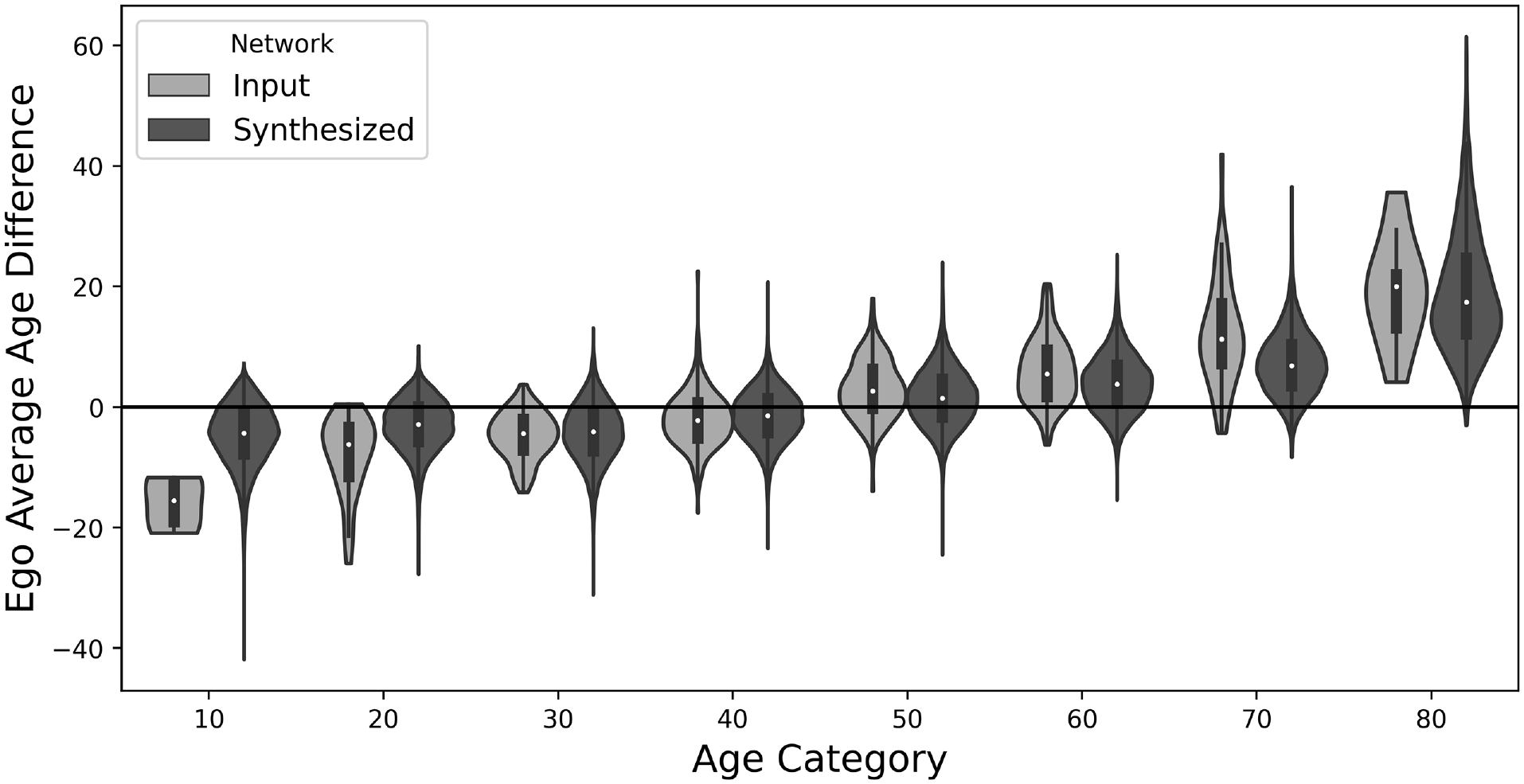
Average ego-centric age homophilies. For readability, only nodes with degrees of 10 or more are included (75% of the population).

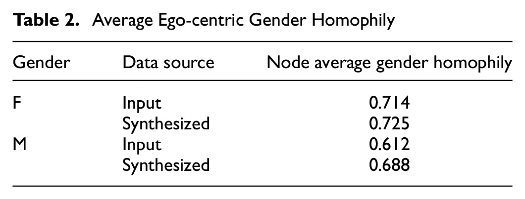
This equilibrium is further observed in Table 2. Perhaps because of sampling biases—61% of the egos in the snowball sample identify as female—on the whole, females in the snowball data exhibit a stronger tendency toward gender homophily. In a more balanced population—the synthetic population is 51% female—this means that, while the female agents can roughly match their homophily, the matching algorithm compensates by having males reach a similar gender homophily. This reinforces the need for repeated draws of the model, as well as the impact of the double-blind matching, as reaching this equilibrium, or even every agent achieving their degree goal under the input homophilies, is not possible from a single draw.

Table 2.

Average Ego-centric Gender Homophily

Gender	Data source	Node average gender homophily
F	Input	0.714
F	Synthesized	0.725
M	Input	0.612
M	Synthesized	0.688

Geographical Distance Distribution Matching

Overall, the approach to geographical distance formation reliably replicates the expected distribution. Figure 7 demonstrates the realized distribution of geographical distances between connected agents for the entire social network compared with the snowball data. 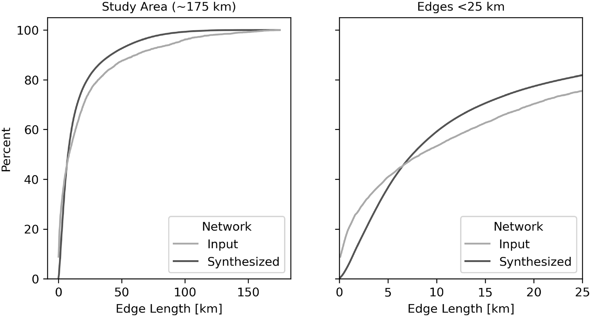There is a slight under-representation of edges under 5 km as the basic power law formulation cannot be sensitive to distances smaller than its scale parameter, $x_{0}$ , which was set as 1.5 km, without causing its probability integral to diverge. Additionally, the synthetic distribution approaches 100% earlier than the snowball data, though this is likely an edge effect, given that only agents near opposite borders of the study area can form the longest connections, making these matches unlikely both to occur and subsequently to pass the probability check.

Figure 7.

Edge length distribution for synthetic population.

Clique Formation and Social Network Structure

The initial triadic closure methodology provides a basic mechanism for clique formation. Roughly 82% of agents have at least one clique in the full social network, though the method significantly overforms small cliques compared with the input data, as seen in Table 3. This is largely a function of adding a single member to a clique being exponentially unlikely, given the iterative and probabilistic nature of the algorithm.

Table 3.

Clique Formation Metrics for the Synthesized Social Network

Clique size	Input, %	Synthesized, %	Input count	Synthesized count
3	33.0	36.9	608	202,219
4	22.8	28.5	420	155,755
5	12.0	18.3	221	100,415
6–10	25.5	16.1	470	88,032
11–15	5.2	0.2	95	949
16–20	1.1	0.0	21	7
21+	0.5	0.0	9	0

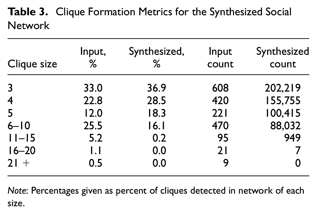
Note: Percentages given as percent of cliques detected in network of each size.

Despite this tendency toward smaller cliques, the social network still demonstrates significant attributes of a well-connected social network. The social network has a transitivity of $0.169$ , which is just at the lower range of the datasets gathered by Mayer and Puller ( 12 ), which ranged from 0.17 to 0.27. These datasets were collected via Facebook within university campuses in the United States and, notably, the larger the social network, the closer that the transitivity is to the bottom end of that distribution. To pick the extremes of the 10 social networks, that with the most nodes (9,299) had the smallest clustering coefficient (0.17), while that with the fewest (820) had the largest clustering coefficient (0.27). It is then potentially reasonable for our social network to have a relatively low transitivity on this scale, just given its size and the percentage of the connections formed outside of the clique search mechanism.

A final metric on the structure of the synthesized social network comes from the eccentricity or, as more commonly understood, the “degrees of separation” ( 37 ). For a graph node, the eccentricity is the “longest shortest path” to any other node in the network. Ignoring the nine disconnected dyads, the greatest eccentricity—the network diameter—is 10, which occurs for $0.8$ % of agents with a degree of one (32 agents total) and is otherwise unobserved. It is computationally expensive to calculate a full eccentricity distribution, but, for a 10% sample of the social network proportionally sampled across all degrees, the average eccentricity is $7.83$ . This leaves us a little wider than the perfect “six degrees of separation” social network, but it does suggest that small-world effects could be observed in this social network ( 18 ).

Scenario Application

The three scenarios—epidemic spread without social network, with pair-wise coordinated destination and with clique coordinated destination—are compared. The main hypothesis is that the total number of infected persons would not vary, as agents perform the same number of activities. But the spatial and temporal distribution is expected to be affected by the presence of social networks and coordinated destination choice. For example, we would be able to capture the outbreak better in recreational areas and large shopping areas; reducing contact at such hotspots may be more sensitive to interventions than limiting social contacts in general. The types of destinations studied are Home, Work, Education, Shopping, Recreation, Public Transit, Other, and Nursing, which refers to nursing homes.

When pair-wise coordinated travel rules were applied in MITO in the Friends scenario, 57% of trips had coordinated destinations. This means 57% of trips were coordinated with a friend. With clique-based coordinated destination in the Cliques scenario, 29% of trips were coordinated with a friend while 33% were coordinated with a clique, meaning in a group of three or more. Figure 8 shows the percentage share of trips by group size.

Figure 8.

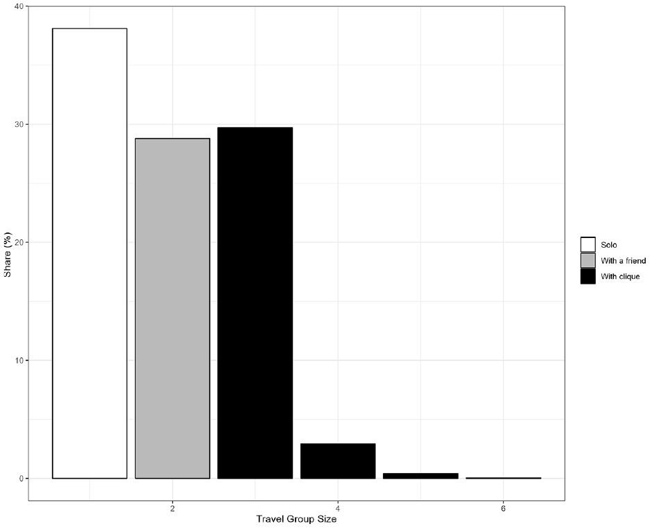
Coordinated destination group size.

Figure 9 shows the EpiSim results for total infected curve for the Munich region for each of the three scenarios. As expected, the total number of infections does not vary significantly between each scenario. The trajectory and the peak of the graph are only slightly staggered.

Figure 9.

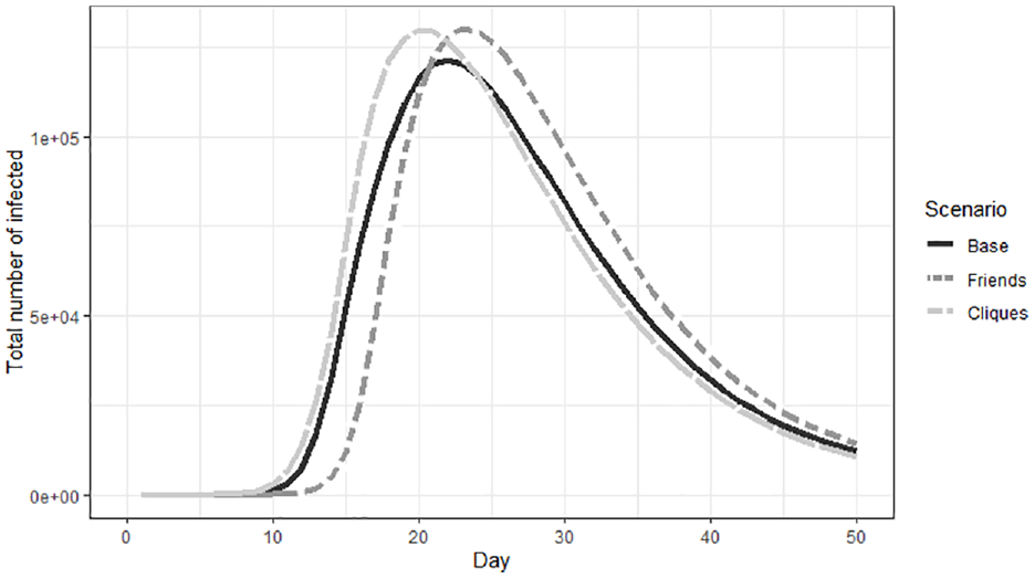
Number of infections from day 1 to day 50.

What is telling is the breakdown of infection events by activity location type. Figure 10 shows the proportion of infection events from clique travel (black), from traveling with a friend (dark gray), and between strangers (light gray). Note that infection events at the Home, Work, and Education locations are infections between household members, work colleagues and schoolmates respectively. The proportion of infection from social network ties increased for the Cliques scenario compared with the Base and Friends scenarios. In total, Friends had 12% of all infection events from social contacts, while Base had 13%: 7% from paired trips and 6% from clique trips. This effect is especially prominent for the Other, Recreation, and Shopping activity locations. The addition of coordinated destination choice captures how non-essential leisure activities may be conducted together with friends, and captures the disease transmission that may happen as a result. Without coordinated destination, agents would seldom meet others in their friendship social network, only family, work colleagues, and schoolmates.

Figure 10.

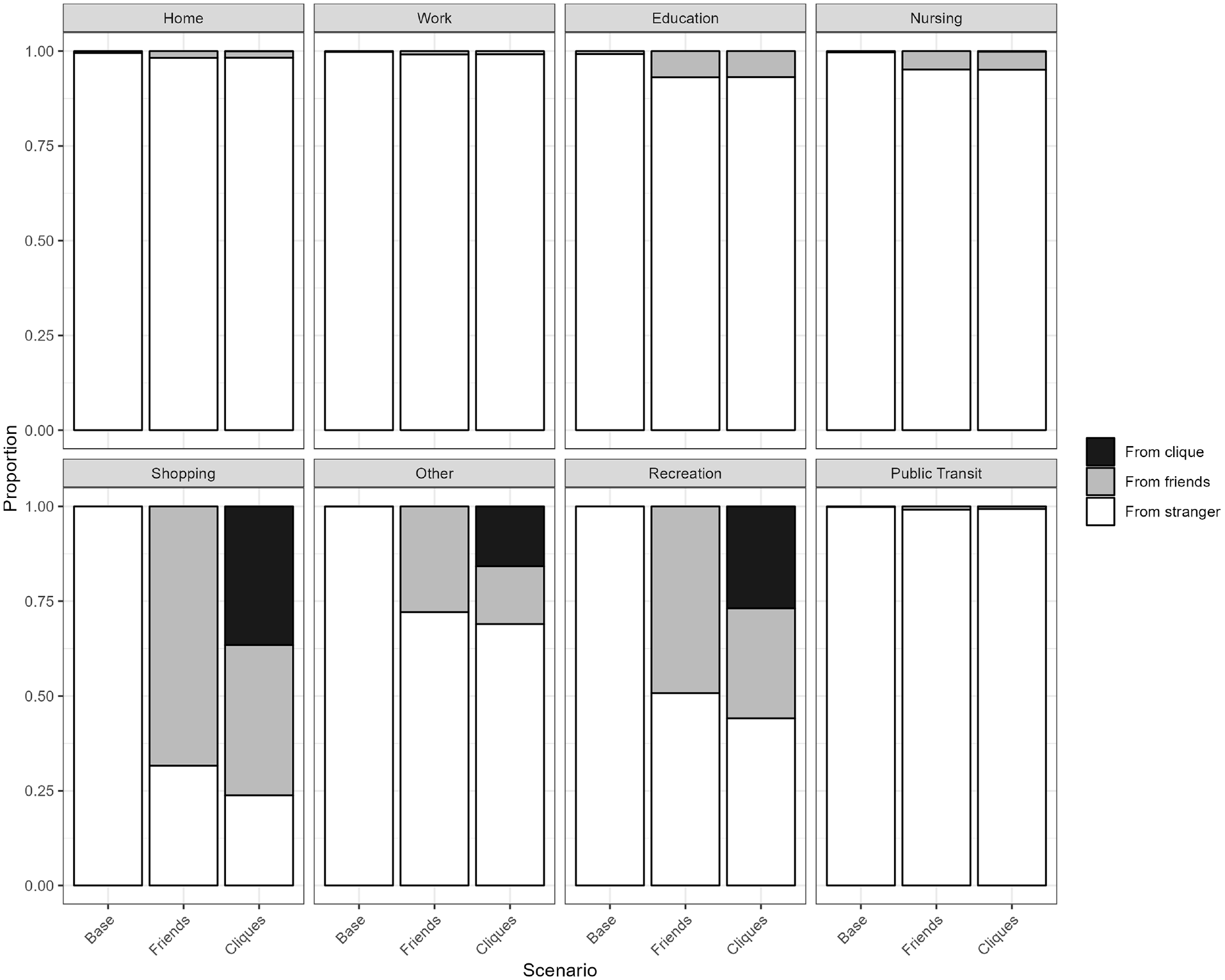
Number of infections by infection location and social network status.

We zoom in on the first 21 days of the epidemic outbreak in Figure 11. This figure shows the day-by-day number of infection events for each scenario. In addition, the figure shows the proportion of infection events from social network and from strangers. At this more micro-temporal scale, we see that the clique-based coordinated destination scenarios have a quicker start compared with the other scenarios. However, the Friends scenario is the slowest. This may be because the cliques enable a higher concentration of people in certain locations compared with the other scenarios. Though the share of infections from social network contacts may be small, keep in mind that the majority of activity time is spent at home, work, and education, which are not explicitly included in our friendship social network.

Figure 11.

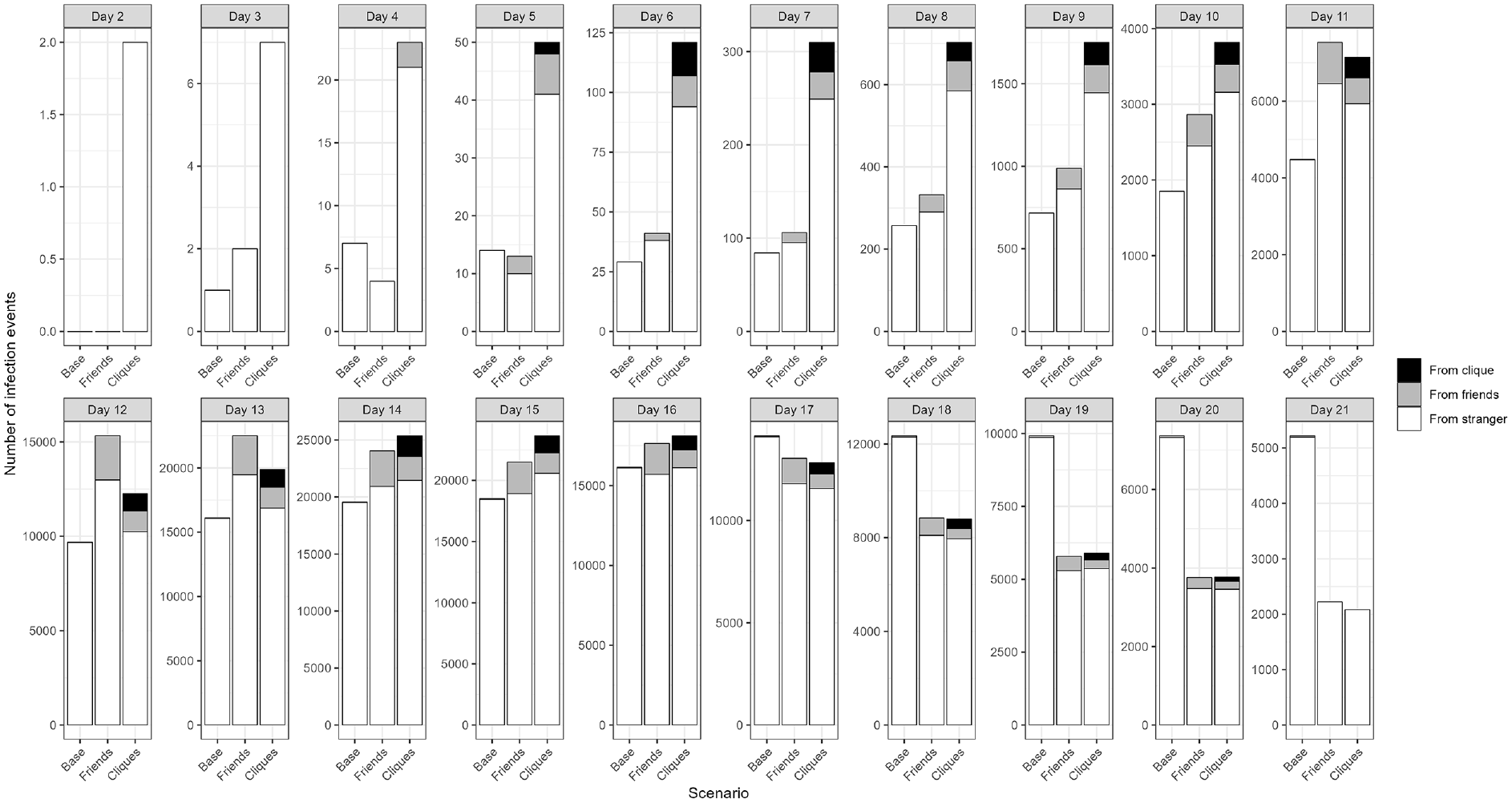
Daily number of infections.

Table 4 shows the percentage of infection from each activity location type and the share of infection from social network contacts per infections at this location. The addition of social networks has increased the share of infections that come from social network ties. The percentage of infection from social network contacts per number of infections varies by activity purpose. The majority of infections happen at Home, Work, and Education locations between household members, colleagues, and schoolmates. The effect of an additional friendship network is seen for leisure activity locations. For example, in Friends and Cliques scenarios, infections from recreation only account for <2% of total infections, because the frequency of recreation acts is rather low. However, social network ties account for over 50% of infections occurring during these acts, as seen in Table 4 and Figure 10.

Table 4.

Share of Infection Events by Infection Location

Location	Scenario
	Base (%)	Friends (%)	Cliques (%)
Home	45 (0.50)	43 (1.7)	43 (1.7) [0.02]
Work	10 (0.15)	9.5 (0.85)	9.3 (0.78) [0]
Education	8.4 (0.71)	7.9 (7.0)	7.9 (6.8) [0]
Nursing Home	1.2 (0.28)	1.2 (5.6)	1.2 (4.8) [0.11]
Shopping	0.04 (0)	0.1 (60)	0.11 (40) [37]
Other	32 (0.05)	34 (28)	34 (15) [16]
Recreation	0.96 (0)	1.6 (50)	1.9 (29) [27]
Public transit	2.8 (0.15)	2.7 (0.90)	2.7 (0.63) [0.02]

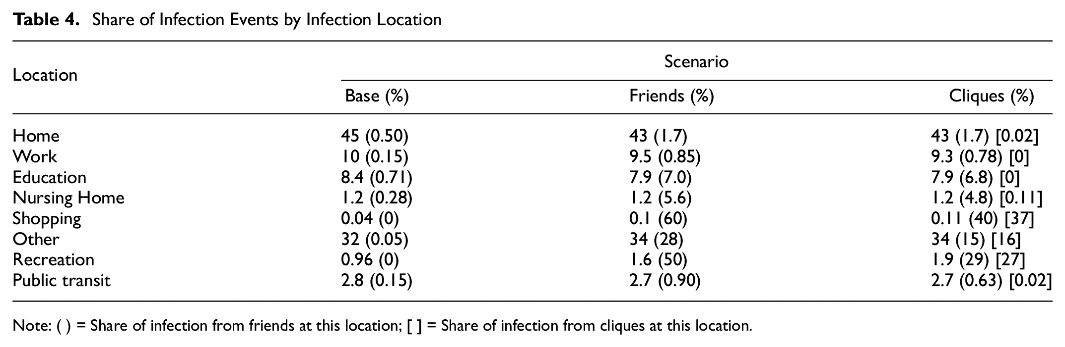
Note: ( ) = Share of infection from friends at this location; [ ] = Share of infection from cliques at this location.

Outlook

This paper presents a scalable method for generating a complete and consistent synthetic social network from a synthetic population with relevant socio-demographic and geospatial characteristics based on a small, ego-centric social network data sample. The generated network demonstrates homophily matching and uses triadic closure to generate small cliques and a network structure resembling other social networks.

Furthermore, the social network was combined with an agent-based travel forecast model and epidemic spread model to see possible effects on epidemic spread patterns. As a first result, our social network and coordinated travel rules demonstrate that social network-influenced travel has some influence on disease spread patterns. Such connections can affect how fast and where the disease spreads.

The value of this methodology is in its ability to produce a geospatially anchored social network with realistic characteristics for downstream travel modeling. The travel demand model was able to utilize the network’s clique structure to capture joint travel behavior of larger groups. This in turn had a marked effect in the epidemic model, hastening its progression and changing its spread pattern. An obvious application would be to use such cliques and clique-based travel behavior to capture the impact of possible super-spreader events during an epidemic.

Future research should focus on implementing a more comprehensive joint travel logic based on social network connections in the travel demand model, as the scenarios with coordinated travel showed a marked effect on epidemic spread compared with those without. A possible next step is inclusion of joint mode choice and travel, as 45% of trips in Germany were performed with at least one companion ( 38 ). A more robust joint decision framework requires further travel behavior analysis to assess how social networks influence joint travel decisions. The joint travel destination choice has not been validated, and in future should be improved via available empirical data.

Another angle for refinement is the social network. The introduction of heterogeneity in homophily is a strong feature, but the segment implementation is largely an artificial heuristic that is a useful way to sort the data; future iterations will likely replace this with a continuous distribution for age differences and conditional probabilities for gender homophily within that distribution. Additionally, the current implementation under-represents neighborhood connections (< 5 km) because of the mathematics of the scale-free probability distribution; mechanisms to encourage edge formation at smaller distances are necessary. Finally, while the triadic closure methodology does perform well to create near-small-world dynamics, a more explicit and tuneable approach to generate larger cliques and increase transitivity may be necessary. As one of the anonymous reviewers rightfully pointed out, religious groups may provide very strong social ties, and should be explored with sufficient relevant data in further research.

Nevertheless, this research provides a key snapshot of the role that social networks can play in travel demand modeling and indicates how further understanding of these networks can broaden the horizons of such models. Just as agent-based travel models turned out to be the perfect environment in which to run a contact-tracing epidemic model like EpiSim, these models provide a simultaneously complex and grounded platform from which to analyze and synthesize social networks. Adapting abstract social network generation algorithms, which are often built abstracted networks, to replicate the kind of networks hinted at in the snowball data is highly challenging, but also potentially the best framework in which to consider the success of such algorithms. A realistic social network will lead to realistic joint travel models, which will then allow us to capture a more complete picture of how people truly move about their surroundings. This research has already shown how this can be applied to draw out the impact of social networks on epidemic spread and it promises to take us anywhere that we can think of, as long as we’ve got a friend.

Footnotes

Acknowledgements

The authors would like to acknowledge the anonymous reviewers for their careful and critical assessment of our work, which has improved the quality of the paper.

Author Contributions

The authors confirm contribution to the paper as follows: study conception and design: R. Moeckel, A. Moreno, Q. Zhang, G. Hannon, J. Ji; data collection: J. Ji, G. Hannon, Q. Zhang; analysis and interpretation of results: G. Hannon, J. Ji, Q. Zhang; draft manuscript preparation: G. Hannon, J. Ji. All authors reviewed the results and approved the final version of the manuscript.

Declaration of Conflicting Interests

The author(s) declared no potential conflicts of interest with respect to the research, authorship, and/or publication of this article.

Funding

The author(s) disclosed receipt of the following financial support for the research, authorship, and/or publication of this article: The research was funded by the German Research Foundation (DFG) under the research project TENGOS: Transport and Epidemic Networks: Graphs, Optimization and Simulation (Project number 458548755).

ORCID iDs

Joanna Yuhang Ji

Ana Tsui Moreno

Rolf Moeckel

References

Kim

Rasouli

Timmermans

H. J.

Social Networks, Social Influence and Activity-Travel Behaviour: A Review of Models and Empirical Evidence. Transport Reviews, Vol. 38, 2018, pp. 499–523. https://doi.org/10.1080/01441647.2017.1351500.

Kowald

Axhausen

Focusing on Connected Personal Leisure Networks: Selected Results from a Snowball Sample. Environment and Planning A: Economy and Space, Vol. 44, No. 5, 2012, pp. 1085–1100. https://doi.org/10.1068/a43458.

Arentze

Kowald

Axhausen

A Method to Model Population-Wide Social Networks for Large Scale Activity-Travel Micro-Simulations. Presented at 91st Annual Meeting of the Transportation Research Board (TRB 2012), Washington, D.C., National Academy of Sciences, Washington, D.C., January 22–26, 2012. https://doi.org/10.3929/ethz-b-000038374.

Dubernet

Explicitly Correlating Agent’s Daily Plans in a Multiagent Transport Simulation: Towards the Consideration of Social Relationships. Doctoral dissertation. ETH Zurich. 2017. https://doi.org/10.3929/ethz-b-000165685.

Sun

Axhausen

K. W.

Lee

D. H.

Cebrian

Efficient Detection of Contagious Outbreaks in Massive Metropolitan Encounter Networks. Scientific Reports, Vol. 4, 2014, pp. 1–6. https://doi.org/10.1038/srep05099.1401.2815.

Feng

Shen

Tam

Yin

Zhao

Modeling Epidemic Spreading Through Public Transit Using Time-Varying Encounter Network. Transportation Research Part C: Emerging Technologies, Vol. 122, 2021, p. 102893. https://doi.org/10.1016/j.trc.2020.102893.

Bóta

Gardner

L. M.

Khani

Identifying Critical Components of a Public Transit System for Outbreak Control. Networks and Spatial Economics, Vol. 17, No. 4, 2017, pp. 1137–1159. https://doi.org/10.1007/s11067-017-9361-2.

Hajdu

Bóta

Krész

Khani

Gardner

L. M.

Discovering the Hidden Community Structure of Public Transportation Networks. Networks and Spatial Economics, Vol. 20, No. 1, 2020, pp. 209–231. https://doi.org/10.1007/s11067-019-09476-3.1801.03857.

Müller

S. A.

Balmer

Charlton

Ewert

Neumann

Rakow

Schlenther

Nagel

Using Mobile Phone Data for Epidemiological Simulations of Lockdowns: Government Interventions, Behavioral Changes, and Resulting Changes of Reinfections. medRxiv, 2020.07.22. https://doi.org/10.1101/2020.07.22.20160093; http://medrxiv.org/content/early/2020/07/24/2020.07.22.20160093.abstract.

10.

Metzler

Miettinen

HyGen: Generating Random Graphs with Hyperbolic Communities. Applied Network Science, Vol. 4, No. 1, 2019, p. 53. https://doi.org/10.1007/s41109-019-0166-8.

11.

Alba

R. D.

Moore

Elite Social Circles. Sociological Methods & Research, Vol. 7, No. 2, 1978, pp. 167–188. https://doi.org/10.1177/004912417800700204.

12.

Mayer

Puller

S. L.

The Old Boy (and Girl) Network: Social Network Formation on University Campuses. Journal of Public Economics, Vol. 92, No. 1, 2008, pp. 329–347. https://doi.org/10.1016/j.jpubeco.2007.09.001.

13.

Asikainen

Iñiguez

Ureña-Carrión

Kaski

Kivelä

Cumulative Effects of Triadic Closure and Homophily in Social Networks. Science Advances, Vol. 6, No. 19, 2020, p. eaax7310. https://doi.org/10.1126/sciadv.aax7310.

14.

McPherson

Smith-Lovin

Cook

J. M.

Birds of a Feather: Homophily in Social Networks. Annual Review of Sociology, Vol. 27, No. 1, 2001, pp. 415–444. https://doi.org/10.1146/annurev.soc.27.1.415.

15.

Leskovec

Krevl

SNAP Datasets: Stanford Large Network Dataset Collection. 2014. http://snap.stanford.edu/data.

16.

Mok

Wellman

Did Distance Matter Before the Internet? Interpersonal Contact and Support in the 1970s. Social Networks, Vol. 29, 2007, pp. 430–461. https://doi.org/10.1016/j.socnet.2007.01.009.

17.

Illenberger

Nagel

Flötteröd

The Role of Spatial Interaction in Social Networks. Networks and Spatial Economics, Vol. 13, No. 3, 2013, pp. 255–282. https://doi.org/10.1007/s11067-012-9180-4.

18.

Watts

D. J.

Strogatz

S. H.

Collective Dynamics of “Smallworld” Networks. Nature, Vol. 393, No. 6684, 1998, pp. 440–442. https://doi.org/10.1038/30918.

19.

Robins

Exponential Random Graph (p*) Models for Social Networks. Springer, New York, NY, 2009, pp. 8319–8333. https://doi.org/10.1007/978-0-387-30440-3_494.

20.

Snijders

T. A.

van de Bunt

G. G.

Steglich

C. E.

Introduction to Stochastic Actor-Based Models for Network Dynamics. Social Networks, Vol. 32, No. 1, 2010, pp. 44–60. https://doi.org/10.1016/j.socnet.2009.02.004.

21.

Granovetter

M. S.

The Strength of Weak Ties. American Journal of Sociology, Vol. 78, No. 6, 1973, pp. 1360–1380.

22.

Van den Berg

Arentze

Timmermans

Location-Type Choice for Face-to-Face Social Activities and Its Effect on Travel Behavior. Environment and Planning B: Planning and Design, Vol. 37, 2010, pp. 1057–1075. https://doi.org/10.1068/b36019.

23.

Moore

Carrasco

J. A.

Tudela

Exploring the Links Between Personal Networks, Time Use, and the Spatial Distribution of Social Contacts. Transportation, Vol. 40, 2013, pp. 773–788. https://doi.org/10.1007/s11116-013-9467-4.

24.

Arentze

T. A.

Timmermans

H. J.

A Need-Based Model of Multi-Day, Multi-Person Activity Generation. Transportation Research Part B: Methodological, Vol. 43, 2009, pp. 251–265. https://doi.org/10.1016/j.trb.2008.05.007.

25.

Ettema

Arentze

Timmermans

Social Influences on Household Location, Mobility and Activity Choice in Integrated Micro-Simulation Models. Transportation Research Part A: Policy and Practice, Vol. 45, 2011, pp. 283–295. https://doi.org/10.1016/j.tra.2011.01.010.

26.

Han

Arentze

Timmermans

Janssens

Wets

The Effects of Social Networks on Choice Set Dynamics: Results of Numerical Simulations Using an Agent-Based Approach. Transportation Research Part A: Policy and Practice, Vol. 45, 2011, pp. 310–322. https://doi.org/10.1016/j.tra.2011.01.008.

27.

Hackney

Marchal

A Coupled Multi-Agent Microsimulation of Social Interactions and Transportation Behavior. Transportation Research Part A: Policy and Practice, Vol. 45, 2011, pp. 296–309. https://doi.org/10.1016/j.tra.2011.01.009.

28.

Marchal

Nagel

Modeling Location Choice of Secondary Activities with a Social Network of Cooperative Agents. Transportation Research Record, Vol. 1935, No. 1, 2005, pp. 141–146. https://doi.org/10.1177/0361198105193500116.

29.

Ronald

Arentze

Timmermans

Modeling Social Interactions Between Individuals for Joint Activity Scheduling. Transportation Research Part B: Methodological, Vol. 46, 2012, pp. 276–290. https://doi.org/10.1016/j.trb.2011.10.003.

30.

Ronald

Arentze

T. A.

Timmermans

H. J.

New Credit Mechanism for Semicooperative Agent-Mediated Joint Activity-Travel Scheduling: Negotiating with Incomplete Information. Transportation Research Record: Journal of the Transportation Research Board, 2011. 2230: 104–110.

31.

Dubernet

Axhausen

K. W.

Implementing a Household Joint Activity-Travel Multi-Agent Simulation Tool: First Results. Transportation, Vol. 42, 2015, pp. 753–769. https://doi.org/10.1007/s11116-015-9645-7.

32.

Moreno

Moeckel

Population Synthesis Handling Three Geographical Resolutions. ISPRS International Journal of Geo-Information, Vol. 7, No. 5, 2018, p. 174. https://doi.org/10.3390/ijgi7050174.

33.

Moeckel

Kuehnel

Llorca

Moreno

A. T.

Rayaprolu

Agent-Based Simulation to Improve Policy Sensitivity of Trip-Based Models. Journal of Advanced Transportation, Vol. 2020, 2020, pp. 1–13. https://doi.org/10.1155/2020/1902162.

34.

Horni

Nagel

Axhausen

K. W.

(eds.) The Multi-Agent Transport Simulation MATSim. Ubiquity Press, London, 2016. https://doi.org/10.5334/baw.

35.

Swiss Federal Railways. MATSim-Extensions by SBB, 2020. https://github.com/SchweizerischeBundesbahnen/matsim-sbb-extensions.

36.

Hagberg

A. A.

Schult

D. A.

Swart

P. J.

Exploring Network Structure, Dynamics, and Function Using NetworkX. In Proc., 7th Python in Science Conference ( G.

Varoquaux

Vaught

Millman

, eds.), United States Department of Energy Office of Scientific and Technical Information, Pasadena, CA, 2008, pp. 11–15.

37.

Hage

Harary

Eccentricity and Centrality in Networks. Social Networks, Vol. 17, No. 1, 1995, pp. 57–63. https://doi.org/10.1016/0378-8733(94)00248-9.

38.

infas, DLR, IBT, and infas 360. Mobilität in Deutschland, 2018. http://www.mobilitaet-in-deutschland.de/publikationen2017.html.

Applying an Agent-Based Social Network in Travel Forecasting with Effects on Disease Spread

Abstract

Keywords

Literature Review

Social Network Generation

Social Travel Modeling

Epidemic Spread Model

Methodology

Determining Social Network Formation Attributes

Social Network Formation

Travel Demand Model and Rule-Based Coordinated Destination

Epidemic Model Extension

Scenarios

Results and Discussion

Social Network Synthesis

Age and Gender Homophilies

Geographical Distance Distribution Matching

Clique Formation and Social Network Structure

Scenario Application

Outlook

Footnotes

Acknowledgements

Author Contributions

Declaration of Conflicting Interests

Funding

ORCID iDs

References