Sage Journals: Discover world-class research

Abstract

Pedestrian volume at intersections is a key input to transportation processes and is vital for developing pedestrian-centric interventions. Though technological solutions to provide continuous monitoring of intersections and field volume counts do exist, most jurisdictions do not have this technology widely deployed and therefore still require a means of estimating volumes. Conventional estimation methods, such as expansion factor methods or the development of direct-demand (DD) models, are alternatives typically employed by practitioners, but they still require known pedestrian volume data for numerous sites, which are often not readily available for jurisdictions. This work explores the use of ChatGPT-4 Vision (GPT-4V) as a tool to assist jurisdictions in estimating pedestrian volume within intersections. The initial assessment of GPT-4V demonstrated its capability in interpreting satellite images, particularly in ranking sites according to pedestrian activity levels. Subsequently, a method was implemented to rank 48 sites based on pedestrian activity using GPT-4V and satellite images. A linear correlation of 0.73 was achieved between the GPT-4V ranking and the true ranking determined from observed field data. Following that, a method was proposed to combine the GPT-4V site rankings and field volumes collected at selected key intersections to estimate the pedestrian volume at all the sites ranked using GPT-4V. Its performance rivaled (and sometimes surpassed) that of existing conventional methods like DD models, all without the need for complex statistical models or extensive datasets. This simplicity makes the GPT-4V method promising for cost-effective pedestrian exposure estimation. This work also investigates inconsistencies and biases in GPT-4V’s responses.

Keywords

pedestrian volume artificial intelligence ChatGPT vision satellite images direct-demand model

Estimating pedestrian volume at intersections is a crucial aspect for jurisdictions aiming to develop pedestrian-centric strategies and interventions. For instance, the road safety management framework proposed in the Highway Safety Manual ( 1 ) includes a network screening step, which necessitates the calibration of models that rely on exposure as inputs ( 2 – 4 ). Another example is ranking intersections based on pedestrian volume within a jurisdiction. This ranking helps optimize the selection of locations for implementing improvements for pedestrians, such as introducing leading pedestrian intervals or maintaining sidewalks ( 5 , 6 ).

The ability of a jurisdiction to comprehensively estimate pedestrian exposure across intersections depends on the type and quantity of information available in regard to pedestrian volume. The typical approach is to combine pedestrian traffic data from continuous counts (CCs) and short-term counts (STCs). CCs involve long-term monitoring (i.e., over years), enabling the direct estimation of annual indicators such as annual average daily pedestrian traffic (AADPT) and facilitating the understanding of seasonal, daily, and hourly temporal patterns. In contrast, STCs are usually collected for 4–12 h over one or a few days, normally for traffic signal design purposes. Since STCs provide punctual observations of pedestrian traffic, they require expansion to AADPT to account for potential biases related to the day of the week and/or month of the year during collection, which is referred to as the expansion factor method ( 7 – 9 ). One of the main challenges with this approach is the requirement that either a CC or an STC be available for every single intersection in the jurisdiction, which is often difficult and resource intensive to fulfill. To address this data availability issue, practitioners employ direct-demand (DD) models to estimate pedestrian volume at sites lacking count data.

DD models estimate pedestrian volume based on explanatory variables associated with socioeconomic attributes (e.g., number of households and employment density), land-use features (e.g., land use mix and number of retail places), and geometric and operational characteristics (e.g., presence of transit stops and density of four-way intersections). These models can be either locally developed using sites where the pedestrian volume is known ( 10 – 14 ) or spatially transferred from other jurisdictions when there are insufficient pedestrian traffic data for model development ( 15 , 16 ).

The expansion factor method and the use of DD models face challenges in practical applications, primarily related to data availability. For example, the expansion factor method necessitates classifying CC sites into factor groups, where each group exhibits similar pedestrian temporal patterns while differing from patterns across other groups. Expansion factors are then developed for each factor group and applied to STCs. Typically, North American jurisdictions use four to five factor groups ( 17 – 19 ), recommending at least five CC sites per group to enhance expansion optimization ( 20 ), which results in the necessity for 20–25 sites under continuous monitoring. In regard to the development of DD models, previous studies have achieved reasonable models (i.e., R-squared ∼ 0.70) using calibration samples from 50–70 sites ( 4 , 13 , 14 ). To contextualize the availability of pedestrian traffic information, Grossman et al. ( 21 ) surveyed 133 US state, regional, and local transportation agencies and found that one-third did not collect any permanent or temporary pedestrian counts. Furthermore, apart from count data, the expansion factor method and the use of DD models also require access to and expertise in manipulating socioeconomic and land-use Geographic Information System (GIS) information.

Researchers have tried to address data availability issues by implementing innovative methods to estimate pedestrian exposure at intersections. For example, Singleton and Runa ( 22 ) examined the use of pedestrian traffic signal push-buttons as a proxy for pedestrian volume at signalized intersections in Utah, U.S. The authors discovered a correlation of 0.84 between the observed hourly volume per crossing and models utilizing the frequency of times the button was pressed as an explanatory variable. In another line of research, Sobreira and Hellinga ( 16 ) explored enhancing spatially transferred DD models (originally developed in another jurisdiction) by locally calibrating them using the limited pedestrian volume data (fewer than 10 sites) available in the jurisdictions where the models were being transferred. This approach yielded accuracy levels similar to those obtained in the original DD model development. However, the authors used limited sample sizes in their study, necessitating further investigation to validate the method’s potential.

Another research direction for estimating pedestrian exposure involves the employment of artificial intelligence (AI). Many researchers have applied AI methods, such as machine learning and deep learning, to estimate pedestrian volumes based on bus dashcam videos (23) and street-view imagery ( 24 , 25 ). However, a common challenge in these works and in the broader use of AI is the substantial effort required to calibrate complex models. In the context of transportation agencies, this requires personnel with AI expertise. Recently, large language models (LLMs)—a type of AI algorithm—have become accessible to the general public, which may help practitioners with certain tasks by eliminating the need for developing their own AI models. The present work introduces a novel method for estimating pedestrian volume at intersections that relies on the use of readily available LLMs (ChatGPT-4 Vision) to visually assess satellite images.

ChatGPT-4 Vision (or GPT-4V) ( 26 ) is available to ChatGPT Plus users and offers image-to-text functionalities, allowing users to input images for visual assessment and interpretation. From a practical perspective, it is an easy-to-apply tool that can be utilized in a vast number of applications, including those in traffic engineering. For instance, Driessen et al. ( 27 ) tested the potential of GPT-4V in assessing driver road safety risk perception from street view images. GPT-4V and humans scored 210 images based on risk perception, revealing a linear correlation of 0.69. In another application, Huang et al. ( 28 ) utilized GPT-4V to predict pedestrian behavior from street-view images for autonomous driving purposes. Although the authors acknowledged the potential of GPT-4V in this context, they found that other state-of-the-art models produced better results.

Given the challenges of collecting pedestrian volume data across entire jurisdictions—whether through CCs, STCs, or DD models—there is a growing need for innovative, scalable methods. This work explores the potential of GPT-4V to visually assess satellite images as a novel approach for estimating pedestrian volumes at intersections in jurisdictions which have limited pedestrian traffic data available. More specifically, the objectives of this work are to:

Explore GPT-4V’s ability to visually assess satellite images, particularly its capacity to identify various types of land use and traffic elements such as crosswalks and transit stops.

Propose and evaluate a method to rank intersections based on pedestrian activity using GPT-4V and satellite images.

Propose and evaluate a method to integrate the site rankings generated in objective 2 with observed pedestrian volume data from a small number of selected intersections, enabling the estimation of pedestrian volume for all sites. This objective is necessary as GPT-4V currently lacks the capability to correlate extracted features from satellite images with actual pedestrian volumes.

Framework

Figure 1 presents the framework for this work. In line with the proposed objectives, the work is divided into three main steps. The first step involves an exploratory investigation of GPT-4V’s ability to visually assess images, aiming to determine its potential for estimating pedestrian exposure at intersections. The second step applies GPT-4V to rank the intersections based on satellite images. In addition, inconsistencies and potential biases in GPT-4V responses are also evaluated. The final step combines the rankings generated by GPT-4V with field-measured pedestrian volumes at specific sites, enabling the estimation of pedestrian volume at all locations.

Figure 1.

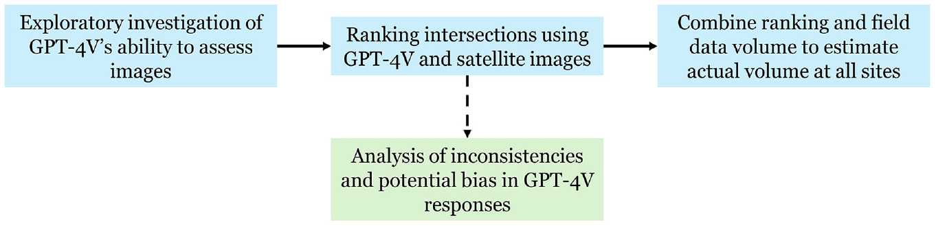
Framework.

Since each step is independent of the others, we have chosen to present the method and results for each step separately. Additionally, the next section describes the datasets used, while the final section presents conclusions and practical applications.

Datasets

Two types of datasets were utilized in this work. The first dataset pertains to pedestrian volume information, which was used to calculate observed volumes at intersections and generate true rankings. The second dataset involves extracting satellite images for intersections where pedestrian data are available, which are then input into GPT-4V.

A total of 48 signalized intersections equipped with CC monitoring systems in the Region of Waterloo, Ontario, Canada, were considered for analysis. Because of the absence of a full year of data in a portion of the intersections, preventing the calculation of AADPTs, the monthly average daily pedestrian traffic (MADPT) for October 2023 was calculated to represent the pedestrian volume at each site. The analyzed sites exhibited a wide range of MADPT, with the following statistics: average = 927; standard deviation = 1,395; minimum = 21; median = 382; and maximum = 7,093.

Satellite images from Google Maps ( 29 ) were extracted from each of the 48 sites using the Google Maps Static API ( 30 ) and the httr package from R ( 31 ). Different types of images can be generated based on multiple factors, including (1) the type of map (a roadmap [standard Google Maps image], satellite view, hybrid view [satellite image with labels], street view, and others) and (2) the zoom level, which ranges from 0 (farthest possible) to 20 (closest possible). Hybrid images were used because of their realistic representation, which aids in identifying land use types, and because they include additional information from labels. The decision on the zoom level was guided by existing DD models, which typically employ land use and socioeconomic variables within a radius of 100–800 m of the intersection center. This led to potential zoom levels of 16–18. Squared images centered at the coordinates of each intersection were extracted, with different zoom levels representing real distances as follows: zoom level 16 = 1,108 × 1,108 m; zoom level 17 = 554 × 554 m; zoom level 18 = 277 × 277 m (these are dimensions for the sites used in this study, but they may vary based on the site’s latitude). After evaluating several images, zoom level 17 was chosen for its perceived optimal balance between the image dimensions and level of detail. This zoom level also allowed for a reasonable number of labeled locations and effectively depicted transportation features, such as transit stops.

We acknowledge the limitations of using 2D satellite images for understanding pedestrian activity. These images do not capture socioeconomic features, such as vehicle ownership rates or household income, which are commonly used as explanatory variables in DD models. Additionally, 2D images cannot detect building heights, making it impossible to consider the “density” factor in the analysis; variables like population and employment density are frequently included in DD models. Therefore, future research could explore the use of different types of images, such as 3D images, and/or combine the images with quantitative measures of the site characteristics (e.g., population density within a given radius) to assist GPT-4V or other models in assessing the images more accurately.

To illustrate this, our initial plan was to create a collage with six images to represent each site: one satellite image showing the land use, one zoomed satellite image depicting the intersection’s geometry (e.g., number of lanes, presence of crosswalks), and four street view images offering a 360-degree perspective. We believed that this approach would better characterize the intersection in regard to pedestrian activity compared with using a single satellite image. However, this plan was undermined by GPT-4V’s limitation of assessing a maximum of 10 images per inquiry (discussed in the next section).

CAN GPT-4V Visually Assess Satellite Images?

The Google Maps satellite images ( 29 ) presented in Figure 2 were used for an initial assessment of GPT-4V’s ability to identify different types of land use and traffic elements. Both sites represented in Figure 2 are from the Region of Waterloo, Ontario, Canada. Figure 2a shows a location with mixed land use, including commercial and residential uses, whereas Figure 2b is predominantly residential.

Figure 2.

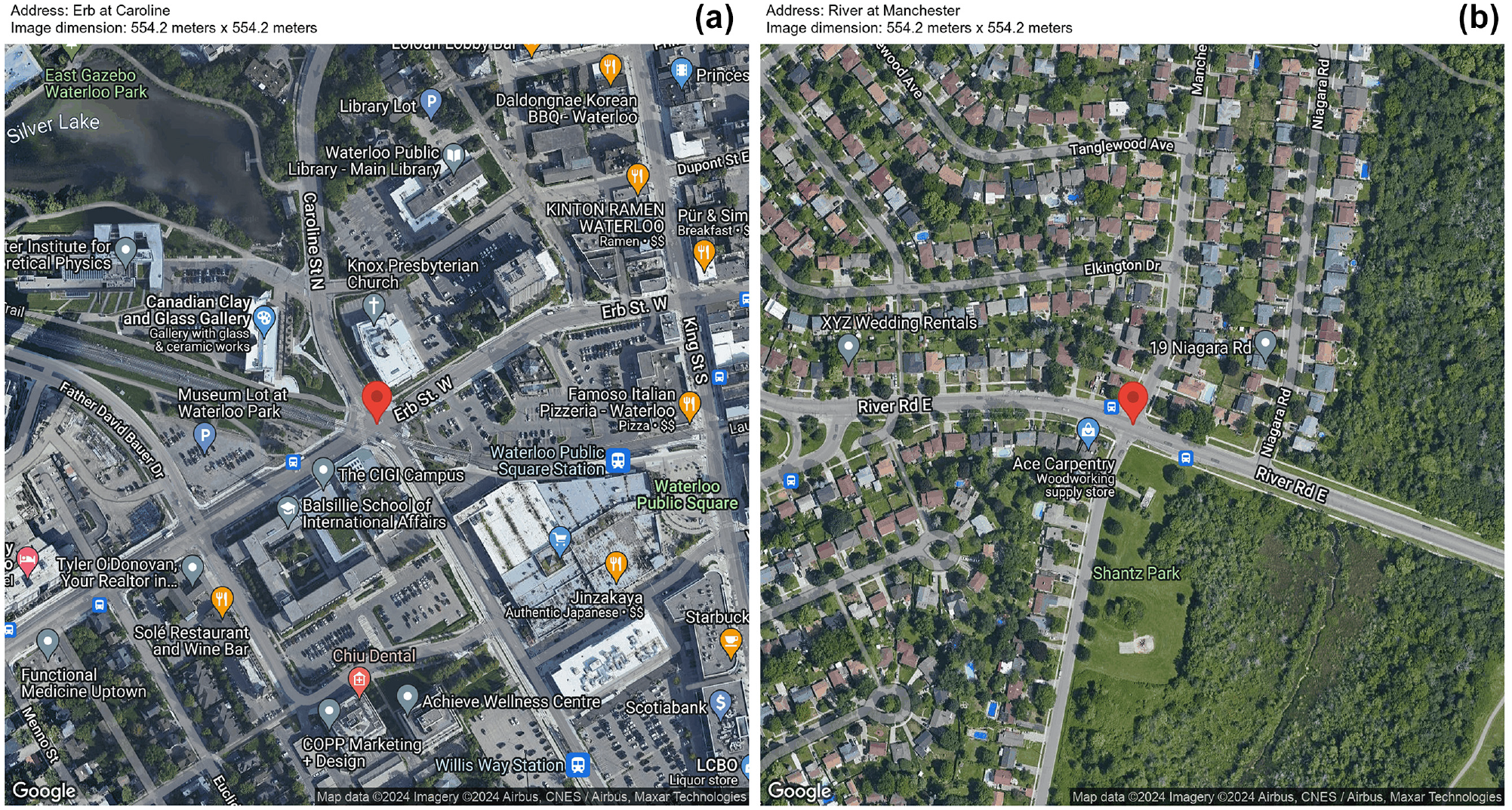
Satellite images used for the preliminary investigation ( 29 ): (a) Erb at Caroline, depicting a scenario with mixed land use; (b) River at Manchester, depicting a scenario with mostly residential land use.

In the initial assessment using Figure 2a, GPT-4V was assigned several tasks. First, it was asked to count the number of commercial places in the image. GPT-4V responded that it was unable to perform a physical count of objects within an image and recommended the use of GIS tools for such tasks. Subsequently, GPT-4V was asked to identify the different types of land use observed in the image. It listed eight types of land use, including commercial, recreational, and residential, providing detailed reasons for each identification. For example, it stated: “Residential: although not as prominently marked, there may be residential use within the area, often integrated with commercial zones in urban settings.” Additionally, GPT-4V was tasked with estimating the percentage of each identified land use type. It provided estimates such as 25% for commercial land use and 20% for transportation spaces like roads and parking lots.

A similar process was conducted using Figure 2b. GPT-4V was able to identify the dominance of residential land use: “From this image, the land use appears to be primarily residential, with single-family homes dominating the landscape …,” indicating that it detected residential places based on the roof’s characteristics. GPT-4V estimated the residential land use to be 80%, while commercial and recreational land uses accounted for 5% and 10%, respectively.

In a subsequent task, GPT-4V was challenged with ranking three images representing sites with varying pedestrian activity levels—high, medium, and low. These images also exhibited notable differences in land use. In response, GPT-4V succinctly described the land use of each location and presented a table ranking the sites from highest to lowest pedestrian activity. For instance, the site identified as having the highest activity was described as a “diverse mix including cultural institutions, a public square, and commercial spaces.” GPT-4V explained the rationale for ranking this site as having the highest activity as follows: “This area is likely to have the highest pedestrian activity throughout the year due to cultural events, daily commercial activity, and the presence of public spaces that encourage foot traffic.” Notably, GPT-4V accurately ranked the sites according to their actual pedestrian activity levels.

These preliminary analyses confirmed the potential of using GPT-4V to rank sites according to pedestrian activity based on satellite images. The subsequent sections delve deeper into exploring how this capability can be applied to a larger context, such as assessing an entire jurisdiction. However, before moving on, it is necessary to highlight some limitations of GPT-4V’s operation:

When this work was developed (between December 2023 and May 2024, using model GPT-4 Turbo), GPT-4V had a couple of input limitations, including (1) a maximum of 30 inquiries within a 3 h period, and (2) a limit of 10 images per inquiry. These limitations add complexity when assessing entire jurisdictions, especially when ranking numerous intersections. They will be further discussed in this work.

GPT-4V exhibits inconsistency. While some level of stochasticity in its answers was anticipated, at times, different responses were observed for the same question. For example, GPT-4V occasionally indicated it could not rank sites because of a lack of visual assessment capability or provided varying estimates for land use percentages from the same images in different inquiries. These types of inconsistencies are another aspect explored in this work.

While GPT-4V can rank sites based on pedestrian activity, it cannot assign pedestrian volumes to the images. This limitation was somewhat expected, considering that the relationship between land use and pedestrian volume (i.e., DD model coefficients) varies across different jurisdictions ( 15 ).

Ranking Intersections: GPT-4V and Satellite Images

This section is divided into three subsections. First, the method for ranking the sites using GPT-4V and satellite images is presented. Second, the results are presented and discussed. Finally, a comprehensive discussion of GPT-4V’s inconsistency and potential bias is provided.

Method

The first step was to create the prompt for the inquiries, an important aspect when working with AI applications ( 32 ). The authors followed a trial-and-error process in the development of the prompt, with the final version of the prompt as follows:

“Each of the files uploaded here represents the satellite image of one intersection (highlighted by the red pin). The header of the images contains the site ID, address, and dimensions of the image. Your task is to rank the intersections in terms of their level of pedestrian activity based on the content of the images (i.e., land use, pedestrian facilities, or other relevant information). Create a descending rank where the first position represents the intersection with the highest pedestrian activity. In your response, provide a table with the ID and Rank of each intersection. Do not include any additional text or information beyond the ranking.”

Two terminologies used to characterize the interactions with GPT-4V are presented. “Failed inquiry” represents an interaction in which images were uploaded to GPT-4V, but it did not provide a final response (i.e., ranking) because of a processing error. Conversely, “successful inquiry” refers to an interaction in which GPT-4V provided a ranking to the inquiry.

The second step involved determining the number of images to be input per inquiry. Ideally, the maximum allowed number of 10 images would have been used. However, it was observed that using this number frequently resulted in failed inquiries. This led to significant delays in interactions with GPT-4V, making it impractical to obtain multiple rankings. Tests were conducted using four, six, and eight images, and it was found that six images proved to be a suitable number for proceeding with the following steps.

A methodological challenge emerged: there are 48 sites to be ranked, but only six sites can be input per inquiry. To address this, a simulation process was proposed. The rationale behind this approach is to rank each site (from 1 = highest activity to 6 = lowest activity) multiple times by considering different arrangements of sites. In the first round of the simulation (k = 1), the 48 sites are randomly divided into eight samples, each containing six sites. These samples are then individually ranked by GPT-4V ( $R_{i, k}$ ). The process is repeated k times, and the average rank score for each site ( ${\bar{R}}_{i}$ ) is calculated using Equation 1. Finally, GPT-4V’s final rank is determined by arranging the 48 sites in ascending order of ${\bar{R}}_{i}$ . We did not implement any specific controls over the generation of the random samples. For future studies, we suggest employing strategies that ensure that all (or as many as possible) site pairs are compared (i.e., each site appears in a sample with every other site at least once).

{\bar{R}}_{i} = \frac{1}{k} \sum_{k} R_{i, k}

(1)

where

$k$ = number of simulation rounds

$R_{i, k}$ = GPT-4V rank associated with site $i$ in round $k$

${\bar{R}}_{i}$ = average rank score for site $i$

The final step involves defining the parameter k. A higher value of k implies more interactions between different sites, potentially resulting in a higher-quality final ranking. However, an increase in k also leads to increased time costs. For this work, k was set at 15, aiming to balance the number of simulation rounds and the time required to interact with GPT-4V. For context, we were able to obtain approximately 50 successful inquiries per day, considering GPT-4V’s usage limit and the frequency of failed inquiries.

In an additional analysis not included in this work, we observed that low values of k (between 1 and 5) resulted in poor and highly variable linear correlations between GPT-4V and true rankings. At around k = 8–10, the correlation stabilized at levels similar to those achieved at k = 15. Our point is that the number of sites analyzed and the number of images input per inquiry affect the k required for achieving stable and accurate results. Future applications should investigate the stability of results when varying k.

Results

Figure 3 displays a scatterplot comparing the true rank obtained from ordering the MADPT of each site with the GPT-4V rank estimated using the process described above. A linear correlation of 0.728 and a mean absolute error (MAE) of 8.125 were achieved in this comparison, suggesting that there is a moderately strong correlation between the GPT-4V ranks and the true ranks. 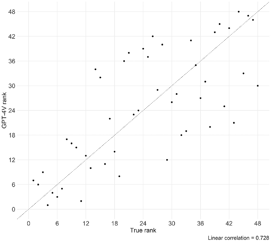It is important to note that there are several sources of error, including the inherent capacity of GPT-4V to analyze satellite images and link them to pedestrian activity as well as the method used to calculate ${\bar{R}}_{i}$ . We were unable to find rank accuracy metrics from other studies in the literature, so we could not compare the performance of GPT-4V’s estimates of sites ranks with rank estimates from other methods. However, in the next section of this paper, we present a proposed method for estimating site MADPT values from the GPT-4V rankings, and we compare the accuracy of those estimates with exposure estimation accuracy from the literature.

Figure 3.

Scatterplot: true rank versus GPT-4V rank.

Figure 4 illustrates the MADPT as a function of the true rank. For the analyzed sites in the Region of Waterloo, the relationship between rank and MADPT is highly nonlinear. The differences between the MADPTs of the top-10-ranked sites are quite large, whereas the differences between the MADPTs for sites ranked 15 or more are small (and probably of less practical significance). Consequently, for practical applications, practitioners should be more concerned about the ranking accuracy of the top-ranked sites than that of the bottom-ranked sites.

Figure 4.

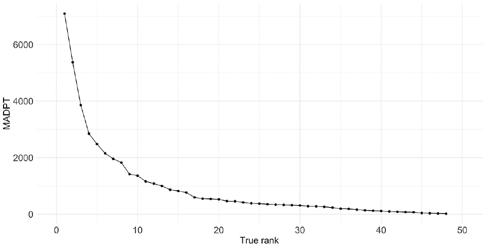
Monthly average daily pedestrian traffic (MADPT) and true rank.

Table 1 presents a confusion matrix between the true and GPT-4V ranks, categorized into bins. For example, the first cell of the first row represents sites correctly placed by GPT-4V into bin 01–10, while the second cell of the first row shows sites belonging to bin 11–20 but incorrectly placed into bin 01–10. Additionally, the MAE of the rank error for each bin of the true rank is presented. As indicated, 41.7% of the sites were placed in the correct bins (highlighted in green cells). Considering adjacent bins as well (highlighted in yellow cells), the performance of GPT-4V improves to 79.2%.

Table 1.

Confusion Matrix: True Rank Versus GPT-4V Rank

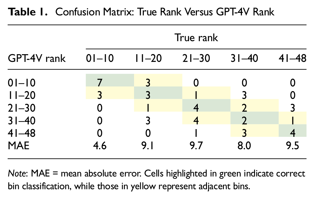
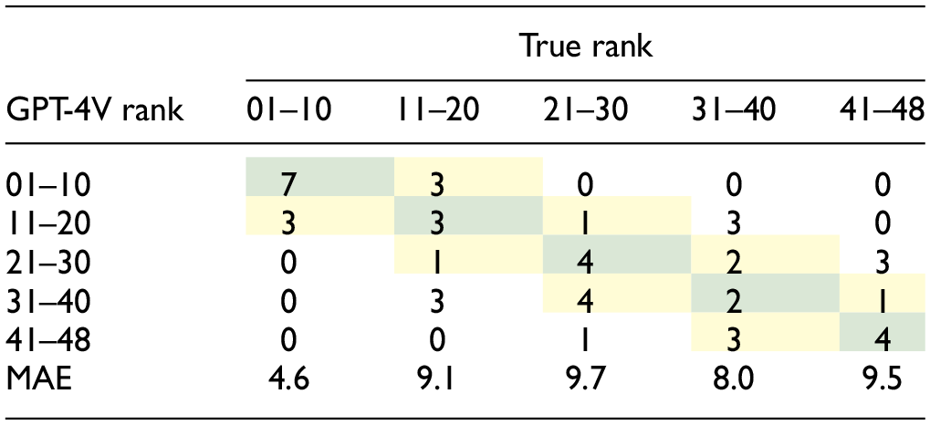
Note: MAE = mean absolute error. Cells highlighted in green indicate correct bin classification, while those in yellow represent adjacent bins.

Table 1 demonstrates that GPT-4V exhibited superior performance in ranking the top sites (bin 01–10) compared with others, as evidenced by the lowest MAE and the highest classification accuracy (seven out of 10 sites) observed in this category. This enhanced performance at the top of the ranking was somewhat expected given the notably higher MADPTs of these sites. It is expected that sites with very high MADPTs will also exhibit distinguished levels of land use and socioeconomic and transportation characteristics, facilitating their identification by GPT-4V. From a practical perspective, this is a good outcome considering the greater concern about sites at the top of the ranking.

Conversely, a higher magnitude of error is observed in the other bins. However, its impact when estimating pedestrian volume is less substantial: inaccuracies in ranking middle- or lower-tier sites result in smaller discrepancies in MADPT compared with misallocations at the top. For instance, the MADPTs for sites at positions 10, 20, and 30 are 1365, 525, and 311, respectively.

Exploring GPT-4V Responses

After interacting with GPT-4V hundreds of times, several concerns about its operation were noted. The most frustrating aspect was the frequent processing errors, in which questions and images were input but GPT-4V failed to provide a final answer (failed inquiries). Though the exact frequency of failed inquiries was not computed, they occurred frequently enough to be a concern.

Another concern was that GPT-4V sometimes generated ranks identical to the order in which the images were input. Given that there are 720 different arrangements for ordering six input images, the likelihood of the images being presented to GPT-V4 in the same order as their true ranks is very low, and therefore we would expect it to be equally rare for GPT-4V to produce a ranking identical to the image order. When such identical rankings were noted, we followed up with GPT-4V to inquire whether we should rely on that ranking or if an error had occurred. GPT-4V responded that “the ranks provided were not based on actual analysis of the content of the images, as it was a placeholder to demonstrate the process …,” indicating that an error had occurred during the processing of images and ranking generation. Therefore, when the resulting ranking matched the image order, that interaction was treated as a failed inquiry.

Additionally, inconsistencies in responses and potential bias toward the order in which images were input were observed, which will be discussed in the following sections.

Inconsistencies in GPT-4V Responses

One noticeable aspect of GPT-4V was its inconsistency across different inquiries. More specifically for this application, GPT-4V derived different rankings when the same dataset of images was input multiple times. An experiment was conducted to demonstrate this.

The experiment involved identifying six sites with varying levels of pedestrian activity. The site selection process consisted of dividing the true ranking into six equal bins and selecting the top site from each bin (i.e., ranks 1, 19, 38, 57, 76, and 95). This site selection process maximized the differences between the levels of pedestrian activity at the sites and theoretically should have made it easier for GPT-4V to rank the sites because of expected visual differences in their land use. Subsequently, the site images were randomly ordered and GPT-4V was asked to rank the sites from 1 to 6. This process was repeated 30 times. Figure 5 illustrates the frequency with which GPT-4V ranked each of the six sites, with the teal-colored column highlighting the true rank.

Figure 5.

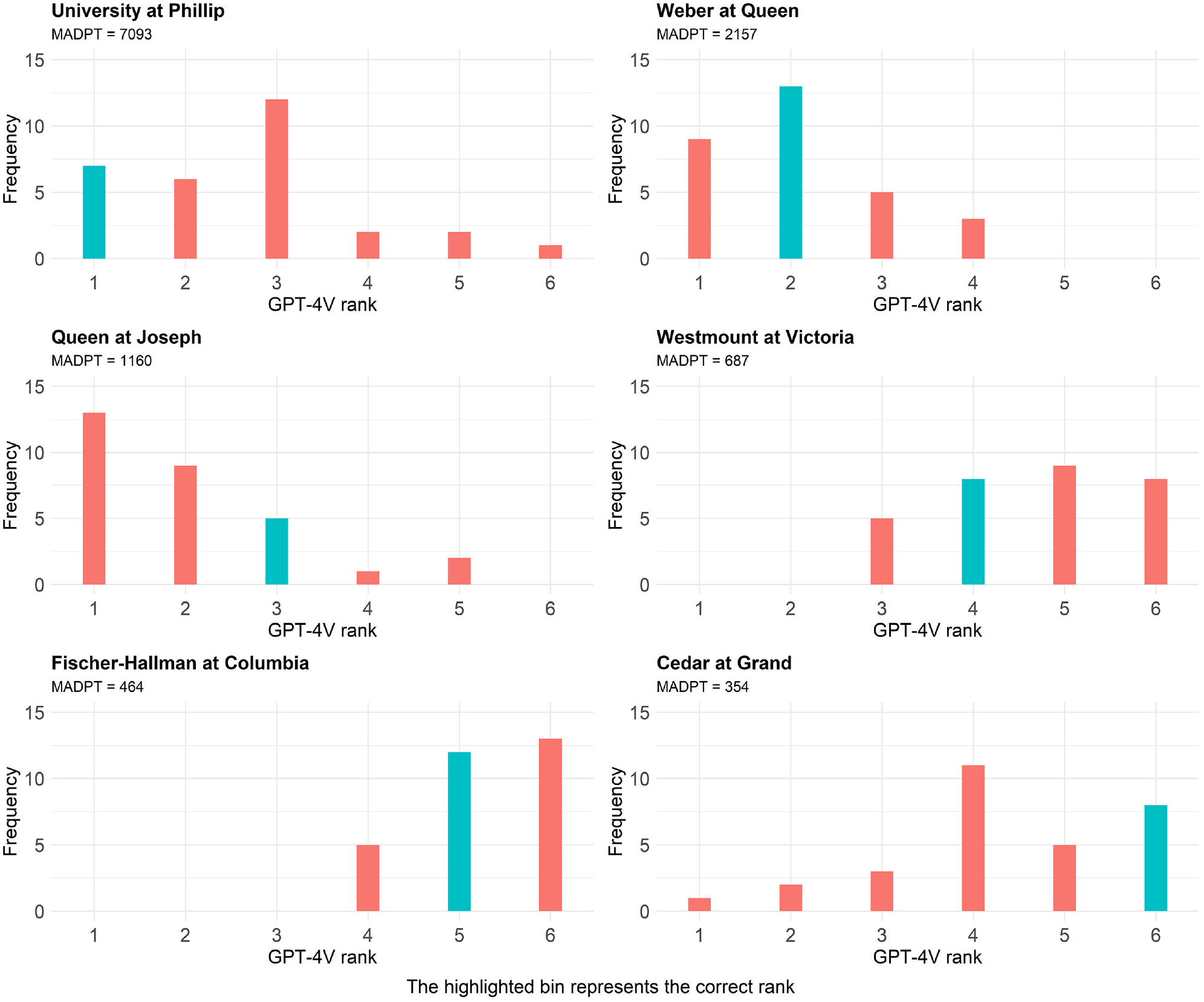
Exploring GPT-4V’s consistency in ranking the same six images.

Figure 5 confirms GPT-4V’s inconsistency in generating different rankings for the same set of images. This outcome was somewhat expected, considering that stochasticity is inherent to GPT-4V’s functioning. This inconsistency is another contributing factor to errors in ranking sites. However, despite the lack of consistency in the rankings, a discernible pattern is observed: sites with true ranks of 1–3 are often ranked at the top of the list, while sites with true ranks of 4–6 are consistently ranked lower.

The combination of having ranks in the same order as the images were input and GPT-4V’s general inconsistency raised suspicions about potential bias in how GPT-4V ranked the sites based on the image order. This led to the following question: does the order in which the images are input affect how GPT-4V ranks them? This question is explored in the next section.

Exploring Potential Bias in GPT-4V Responses

The Friedman test was used to examine potential biases in GPT-4V outcome rankings based on the order in which the images were input. The Friedman test is a nonparametric statistical test used to analyze related samples. It shares similarities with repeated-measures analysis of variance (ANOVA) but focuses on the ranking of measurements rather than the actual measurements themselves. An example is provided to clarify the Friedman test. Consider a scenario where five patients are experiencing back pain and are scheduled to undergo surgery to address the issue. Each patient is asked to numerically rate their pain from 0 to 100 at three different time points: before surgery, 1 week after surgery, and 1 month after surgery. The pain measurements from each patient are ranked from 1 to 3, and then the ranks for each time point are summed across all patients. The Friedman test is applied to determine if there are significant differences in pain ratings across the three time points. The null hypothesis for the Friedman test is that there are no differences in pain ratings between the time points.

The Friedman test was adapted to investigate potential bias arising from the order in which images were input. In this study, 15 rounds of simulation were conducted, with six images input per inquiry. With a total of 48 sites, each round required eight different samples, leading to 120 interactions with GPT-4V in total (15 rounds × 8 samples). In the context of the example above, the interactions can be linked to patients, the order of image input (from 1 to 6) represents the “time points,” and the resulting rank from GPT-4V serves as the measurement. Since the samples were randomly generated (i.e., random image orders), random distributions of ranks by GPT-4V would be expected if there was no bias. In other words, the null hypothesis was expected to hold and not be rejected.

The application of the test, however, resulted in the rejection of the null hypothesis (p value = 0.004), indicating that GPT-4V is biased by the order in which the images are input. The sum of ranks for each image order increased progressively from position 1 (369) to position 6 (477), indicating that GPT-4V tended to rank images that were input first as having higher pedestrian activity (i.e., ranks closer to 1).

The Friedman test result was unexpected given the strong linear correlation between the true ranks and the GPT-4V ranks as presented in Figure 3. To better understand these results, it was decided to investigate each of the 120 interactions with GPT-4V using three indicators to measure the deviation between image order, true rank, and GPT-4V rank. ${\bar{E}}_{IG}$ and ${\bar{E}}_{IT}$ (Equations 2 and 3) represent the deviation between image order and GPT-4V rank and between image order and true rank in each interaction, respectively. Evaluating both indicators simultaneously helps in identifying whether a GPT-4V ranking similar to the image order should be expected or not, given the true ranking. Both indicators vary from 0 to 3, representing cases with identical orders and completely different orders, respectively. An additional indicator, ${\bar{E}}_{TG}$ (Equation 4), is also used to represent the deviation between GPT-4V and true ranks. Although it does not directly contribute to the bias issue, it indicates the ranking accuracy of each interaction.

{\bar{E}}_{IG} = \frac{1}{n} \sum_{j = 1}^{n} | j - G_{j} |

(2)

{\bar{E}}_{IT} = \frac{1}{n} \sum_{j = 1}^{n} | j - T_{j} |

(3)

{\bar{E}}_{TG} = \frac{1}{n} \sum_{j = 1}^{n} | T_{j} - G_{j} |

(4)

where

$n$ = number of images per inquiry (six in this work)

$j$ = image order

$G_{j}$ = GPT-4V rank associated with the image in order $j$

$T_{j}$ = true rank associated with the image in order $j$

Figure 6 shows a scatterplot of the indicators ${\bar{E}}_{IG}$ and ${\bar{E}}_{IT}$ for the 120 interactions with GPT-4V. The color of each dot is associated with its ${\bar{E}}_{TG}$ . Four quadrants (Q1–Q4) were created using the indicators’ midpoint of 1.5. Each quadrant could be interpreted as follows:

Q1: high ${\bar{E}}_{IT}$ and high ${\bar{E}}_{IG}$ (68 interactions). True and GPT-4V ranks are different from the image order. This suggests interactions that are not biased and are probably accurate.

Q2: low ${\bar{E}}_{IT}$ and high ${\bar{E}}_{IG}$ (11 interactions). GPT-4V ranks are different from the image order, but true ranks are similar to the image order. This suggests interactions that are not biased and are probably inaccurate.

Q3: low ${\bar{E}}_{IT}$ and low ${\bar{E}}_{IG}$ (15 interactions). True and GPT-4V ranks are similar to the image order. This suggests interactions that could be biased but are probably accurate.

Q4: high ${\bar{E}}_{IT}$ and low ${\bar{E}}_{IG}$ (26 interactions). True ranks are different from the image order, but GPT-4V ranks are similar to the image order. This suggests interactions that are biased and probably inaccurate.

Figure 6.

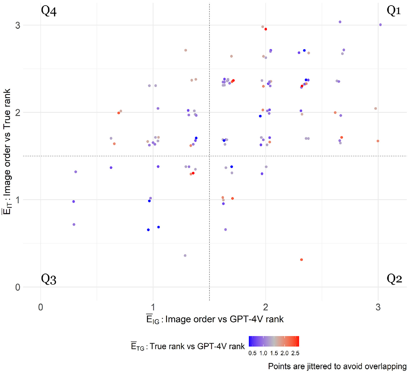
Exploring the bias in GPT-4V’s responses. Q1, Q2, Q3, and Q4 are the quadrants of the scatterplot.

Interactions that fall in quadrants Q3 and Q4 raise concerns about potential bias. It is challenging to definitively state that there is bias in Q3 because the image order corresponds to the true order, and therefore the observation that GPT-4V rankings correspond to the image order can indicate a bias or that the rankings are unbiased and accurate. Conversely, Q4 represents a more severe case of potential bias. While it is known that the true ranks differ from the image order, GPT-4V ranked the sites similarly to how the images were provided.

The Friedman test was conducted again considering two scenarios: (1) sites in Q1 and Q2 and (2) sites in Q1, Q2, and Q3. The null hypothesis was not rejected in either case, with p values of 0.472 and 0.885, respectively. This suggests that the group of interactions in these quadrants is not biased. Consequently, this raised the suspicion that only a portion of the interactions (those in Q4) were biased by the image order.

A detailed investigation was conducted on the interactions in Q4 to evaluate whether the bias was triggered by a specific factor. Initially, the sites and satellite images frequently involved in these interactions were assessed, but no particular pattern was observed. Subsequently, it was decided to repeat some of the interactions in Q4 using the same images and image order. Each interaction was replicated 20 times, and the ${\bar{E}}_{IG}$ was computed. Stochasticity was observed across the different ${\bar{E}}_{IG}$ values, with more interactions occurring in Q1 and fewer in Q4. Despite our efforts, we were unable to identify the reasons for the bias toward image order that affected certain interactions. This bias could be attributed to factors such as GPT-4V’s momentary processing capacity. Notably, these interactions appeared to occur randomly and did not target any specific group of sites, which meant that any bias-related errors were spread across multiple interactions.

In conclusion, it was decided to acknowledge the limitation that approximately 21.6% (26 out of 120 interactions) of the rankings generated by GPT-4V are located in Q4 and may be biased. However, there are reasons to believe that these biased interactions occur randomly; therefore, their error will be diluted among the other interactions, somewhat minimizing the problem, especially when a decent number of simulations are performed.

Estimating Pedestrian Volume From Rankings

The method described in the previous section provides the ranking of sites with respect to the expected level of pedestrian activity at each site. These site rankings could be beneficial for jurisdictions, particularly in selecting locations for pedestrian-centric interventions. However, just knowing the site rankings does not provide an estimate of the pedestrian volume, which could be used for road safety analyses. In this section, a method is proposed to estimate pedestrian volumes based on rankings. Subsequently, the results are presented and discussed.

Method

The proposed method integrates the ranking derived from GPT-4V with the collection of pedestrian volume data from key sites. Figure 7 presents the method, illustrating a case in which a dataset with 16 sites is used. The first step involves splitting the GPT-4V ranking into categories based on percentiles. In Figure 7, four categories were established, which could be interpreted as very high, high, low, and very low pedestrian activity. The second step is to collect field volume data (STC, daily or weekly volume, MADPT, or AADPT) for the sites that represent the category boundaries. For this work, it was assumed that October MADPT data are available for these sites. The third step is to check for inconsistencies in the ranks. In Figure 7, for example, the site ranked as the fourth position has a lower volume than the site ranked as the eighth position, indicating an error in GPT-4V ranking. To rectify this, the positions for the two sites are swapped (i.e., the site originally ranked as fourth is now eighth, and vice versa). The fourth step involves estimating the volume of the sites with unknown volume using the category boundaries. Linear and nonlinear methods were considered and are discussed below.

Figure 7.

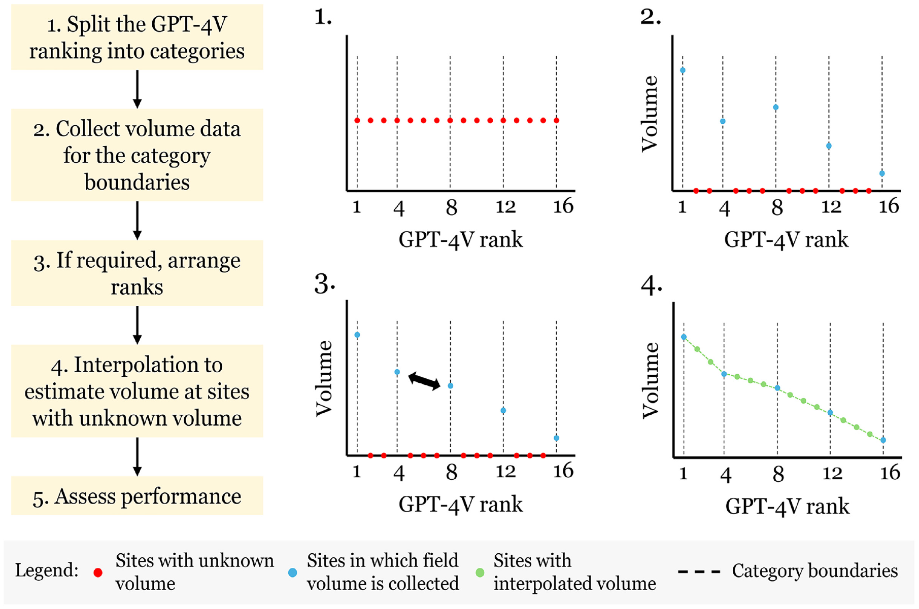
Method to estimate pedestrian volume from rankings.

Linear interpolation was initially employed for all categories: the volume of the sites within each category was predicted considering the boundary volumes and the GPT-4V ranks. However, as can be seen from Figure 4, the pedestrian volumes of the sites at the top of the ranking (i.e., first categories) do not follow a linear distribution. Therefore, a large error was observed when using linear interpolation for these sites. This pattern may be specific to the Region of Waterloo, so it was decided to investigate the volume distribution across sites in three additional jurisdictions: Milton, ON, Canada; Pima County, AZ, U.S.; and Toronto, ON, Canada. Table 2 presents a summary of the pedestrian volume, represented as the AADPT between 2022 and 2023, for each jurisdiction. Note the significant variation in pedestrian activity magnitude across jurisdictions.

Table 2.

Additional Jurisdictions: Descriptive Statistics

		AADPT (2022–2023)
Jurisdiction	Number of sites	Average	Minimum	Maximum
Milton, ON, Canada	38	320	27	1,097
Pima County, AZ, U.S.	87	29	2	2,528
Toronto, ON, Canada	49	12,193	651	30,675

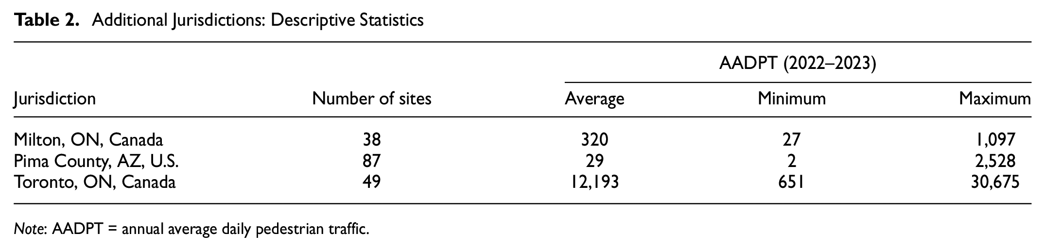
Note: AADPT = annual average daily pedestrian traffic.

Figure 8 displays the scaled volume plotted against its associated percentile, with each jurisdiction represented by a distinct color. Examining the sites in the first quartile, it is evident that Pima County and Waterloo exhibit a nonlinear distribution, Toronto shows a distribution close to linear, and Milton presents a mix of linear and nonlinear distributions. For sites in the other quartiles, distributions close to linear are observed across all jurisdictions.

Figure 8.

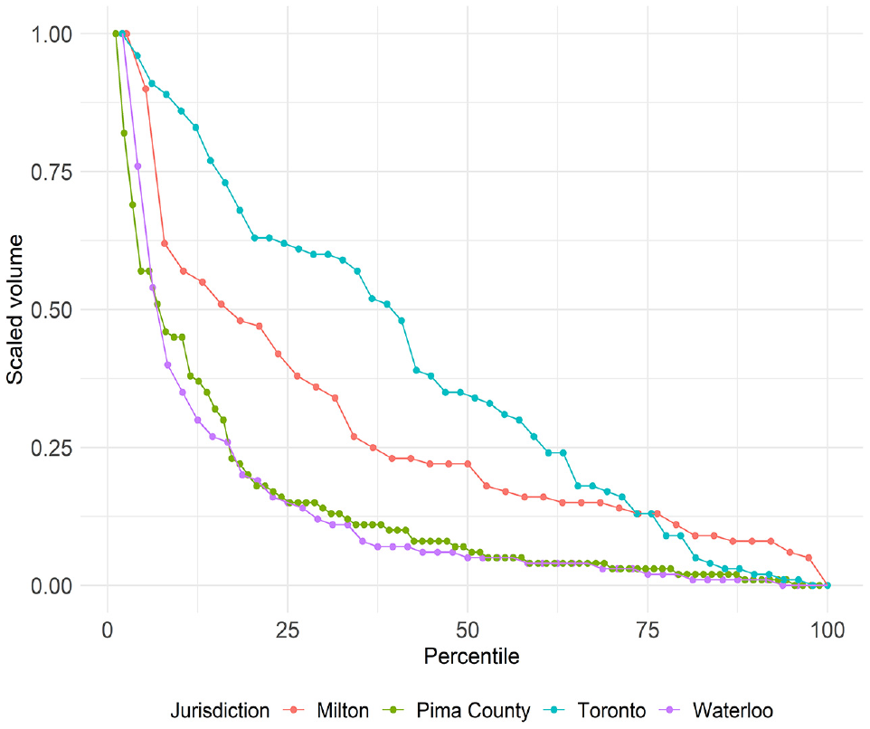
Pedestrian volume distribution across different jurisdictions.

To address the nonlinearity observed in the first category in certain jurisdictions, nonlinear models were developed to predict volume for these sites. Exponential, logarithmic, and polynomial models were calibrated using pedestrian volume observations from the first three boundaries (using all boundaries resulted in poorly fitted curves in the first category). The pedestrian volume (MADPT) served as the dependent variable, while the GPT-4V rank was the independent variable. Initial analysis revealed that the logarithmic model offered the best accuracy and was therefore adopted for this study. In summary, two methods are now used for estimating pedestrian volume at sites with unknown volume: (1) linear interpolation for all categories and (2) a logarithmic model for the first category and linear interpolation for subsequent categories.

From a practical perspective, analyzing the shape of the distribution of the volumes of sites where field volumes were collected (plot 3 from Figure 7) can provide insights into whether the logarithmic model method should be employed. Figure 9 illustrates two different scenarios. If there is a significant difference between the slope of a straight-line fit to the volumes of the first two boundaries and the slope of a line through the other boundaries, the logarithmic model method is recommended (Figure 9a). Otherwise, linear interpolation for all categories is advised (Figure 9b).

Figure 9.

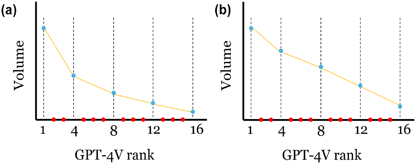
Determining if the logarithmic model or the linear interpolation approach should be adopted in the first category on the basis of field volumes: (a) Logarithmic model method is recommended and (b) Linear interpolation is recommended.

Returning to the method itself (Figure 7), the final step is to assess the performance of the predicted volumes. The MAE is calculated for all sites in the dataset (i.e., those with field or predicted volumes) using Equation 5. Subsequently, the MAE is divided by the average true MADPT (Equation 6) to standardize the performance measurement, making it comparable across jurisdictions with varying levels of pedestrian activity. The mean absolute percent error (MAPE) is also employed (Equation 7).

MAE = \frac{1}{n} \sum_{i = 1}^{n} | Y_{i} - Y_{i}^{'} |

(5)

\frac{MAE}{\bar{Y}} = \frac{MAE}{\frac{1}{n} \sum_{i = 1}^{n} Y_{i}}

(6)

MAPE = \frac{1}{n} \sum_{i = 1}^{n} \frac{| Y_{i} - Y_{i}^{'} |}{Y}

(7)

where

$n$ = number of sites

$Y_{i}$ = true MADPT at intersection $i$

$Y_{i}^{'}$ = predicted MADPT at intersection $i$

$\bar{Y}$ = average true MADPT across all intersections

Results

Figure 10 presents the performance comparison of both the linear interpolation and the logarithmic model methods for different numbers of categories (ranging from 4 to 11). For this analysis, the maximum of 11 categories (resulting in 12 boundaries) was chosen to represent the collection of field volume data for 25% of the 48 sites in the dataset. In the figure, the horizontal dashed line at 0.60 serves as a benchmark performance level based on alternative approaches for estimating pedestrian volume when neither CCs nor STCs are available for all sites within a jurisdiction. One such approach is the local development of DD models, which prior work suggests yield $MAE / \bar{Y}$ values of around 0.60 and 0.65 ( 4 , 11 ). This approach typically necessitates access to 50–70 sites with available pedestrian volume data for model development. Another approach is the local calibration of an existing DD model developed in another jurisdiction. Prior work shows that this approach can provide similar performance to locally developed DD models but requires fewer sites for implementation ( 16 ). There is only a single study that investigated the local calibration of DD models, and it used limited sample sizes. Although it has shown potential for its simplicity and reasonable level of accuracy, further investigation is required to validate this method. Furthermore, a practical limitation to adopting the local calibration approach is the availability of an existing DD model developed in another jurisdiction that has similar characteristics to the target jurisdiction. Both locally developed and calibrated DD model approaches, besides requiring available sites with pedestrian volume data, also depend on the existence and usability of land-use, socioeconomic, and transportation GIS databases, introducing additional complexity to their application.

Figure 10.

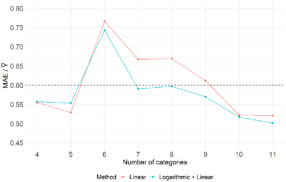
Performance assessment: estimating pedestrian volume from ranks.

The performance shown in Figure 10 for estimating pedestrian volume from GPT-4V ranks is quite promising as it meets, and in some cases surpasses, benchmark approaches, with $MAE / \bar{Y}$ ranging between 0.50 and 0.55 for certain categories. Moreover, this method is simpler to implement compared with DD model approaches: (1) it requires pedestrian volume data for only a few sites; (2) there is no need for land use, socioeconomic, or transportation GIS databases; and (3) it does not involve developing complex statistical models. Instead, it relies on relatively simple tasks, such as extracting satellite images, interacting with GPT-4V, and employing a straightforward method to estimate pedestrian volume at sites with unknown volume.

To provide additional context on GPT-4V’s performance, Table 3 presents the accuracy in regard to MAPE when splitting the GPT-V4 rankings into five categories to identify sites for collecting field volumes and using the logarithmic model for interpolation. The results are compared with an alternative approach that jurisdictions might adopt in the absence of pedestrian data, which involves hiring third-party companies to provide volume estimates based on crowd-sourced data. For instance, StreetLight uses anonymized location data from various mobile apps to estimate pedestrian volume ( 33 ). The results are categorized by volume range to avoid bias toward low-volume sites, and both MAPE metrics are calculated based on MADPT estimates. Except for the first category, the GPT-4V method outperforms the crowd-sourced data approach.

Table 3.

MAPE: GPT-4V Versus StreetLight

Volume range	GPT-4V		MAPE: StreetLight ( 33 )
Volume range	No. of sites	MAPE	MAPE: StreetLight ( 33 )
Low (<150)	23	273	151
Mid-level (150–500)	37	51	89
High (500–1,000)	14	51	82
Very high (>1,000)	27	49	71

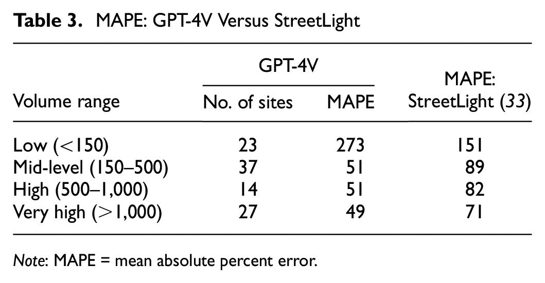
Note: MAPE = mean absolute percent error.

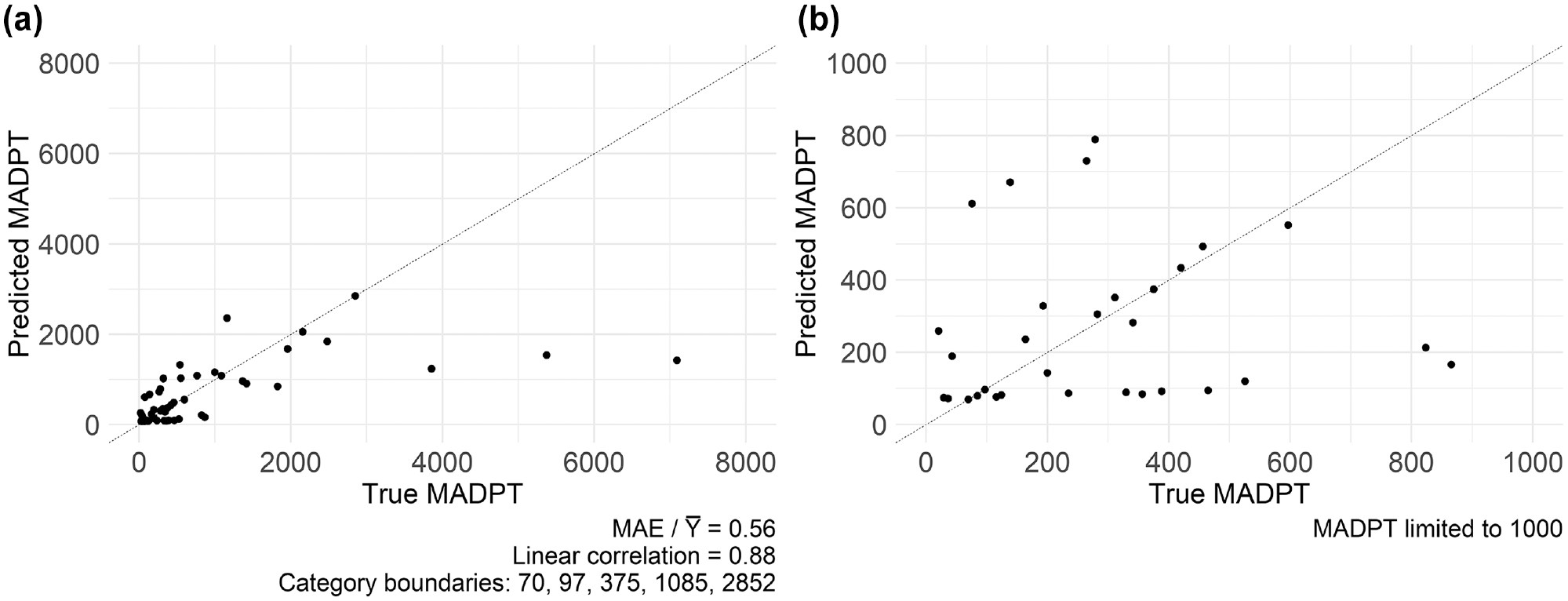
Expanding on a datapoint from Figure 10, Figure 11 showcases the true MADPT versus the predicted MADPT using four categories and the logarithmic model approach. Figure 11a provides an overview of the entire dataset, while Figure 11b focuses on sites with an MADPT lower than 1,000. The proposed method achieved an accuracy performance of $\frac{MAE}{\bar{Y}} = 0.56$ with a strong linear correlation of 0.88. Notably, Figure 11a reveals a significant underprediction for sites at the top of the ranking (high volume). This discrepancy arose as a result of GPT-4V erroneously ranking the site at the top of the true ranking as the fourth position. Consequently, the first category boundary was incorrectly set at 2,852 instead of 7,093, resulting in the underprediction of sites occupying the top three positions in the true ranking. In general, Figure 11b demonstrates instances of accurate predictions but also highlights cases of under- and overprediction resulting from imperfections in the GPT-4V ranking.

Figure 11.

Predicted versus true MADPT using four categories and the logarithmic model approach: (a) all sites; (b) zoomed at sites with an MADPT lower than 1,000.

In regard to performance differences between the linear interpolation and logarithmic model approaches, Figure 10 reveals varying performances across different categories. Notably, the logarithmic model approach demonstrates superior performance in categories 7, 8, and 9, while similar performances are observed in the remaining categories. It was observed that the logarithmic model approach outperformed the linear interpolation approach when sites at the top of the true ranking (positions 1 or 2)—representing sites with extremely high pedestrian volume—were included in the category boundaries. This aligns with expectations, as linear interpolation did not perform well for the first category when there was a significant difference in volume between the first two boundaries.

The shapes of the curves in Figure 10 are somewhat unexpected. One might anticipate a systematic improvement in performance with an increase in the number of categories, but this trend is not observed (categories 4 and 5 are superior to categories 6–9). Additionally, the high magnitude of error in category 6 is atypical. To explore these further, the sites selected to define the category boundaries in these categories were closely examined. It was found that the good performance in categories 4 and 5 and the poor performance in category 6 are linked to specific characteristics of the sites chosen to form the category boundaries. In other words, the results depicted in Figure 10 are specific to the particular final ranking generated by GPT-4V and do not necessarily reflect overall (or populational) performance metrics. To ensure results are not limited by the specificity of the particular ranking generated by GPT-4V, two simulation approaches are proposed and implemented in the next section.

Simulation Approaches

It was demonstrated previously in this work (Figure 5) that GPT-4V is inconsistent and provides different rankings for the same set of images. With this established, it is evident that the results presented in the previous section are subject to randomness. Put differently, if the interactions with GPT-4V were repeated another 120 times, a similar final ranking in regard to general trends would be expected, but individual sites would likely have different ranks. In an ideal scenario, we would replicate the 120 inquiries to GPT-4V multiple times to examine the statistical variation in the results in Figure 10. However, given the large resource requirements associated with carrying out such replications, we decided to pursue two simulation approaches to estimate the statistical variation and obtain more generalizable results.

The first simulation approach relies on the original final ranking generated by GPT-4V but with a different selection of sites that represent the category boundaries (plot 1 from Figure 7). This would represent the shifted positions obtained from new rankings. To implement it, the ranks of the sites at the boundaries were randomly switched with a site that is close to each boundary. For example, when n = 1, an integer from the set {−1, 0, +1} is randomly selected and added to the boundary rank. For instance, if the original boundary rank was 8 and the randomly selected number is −1, then the site ranked 8 is switched with the site ranked 7. This process is repeated separately for each boundary to allow multiple random replications. After completing this procedure for all boundaries, steps 2, 3, and 4 from Figure 7 are conducted as usual. This procedure was carried out for n = 1 and n = 2.

The above simulation process is attractive in that it is intuitive. However, the error that is introduced (the value of n) is arbitrary and uniform across all boundaries. The second simulation approach addresses these two issues by using the observed distribution of rank errors and varies this error across the boundaries. The procedure is outlined below:

Calculate the deviation between the true ranks and the original GPT-4V ranks for all 48 sites. This is the observed distribution of rank errors.

As shown in Figure 3, rank errors are larger when the true rank exceeds 12. To account for this, two distributions of rank errors were created: one for sites ranked between 1 and 12 and another for sites ranked between 13 and 48.

Define an auxiliary variable $V_{i} = T_{i} + ε_{a}$ , where $T_{i}$ is the true rank of site i and $ε_{a}$ is the random error from the error distribution for sites ranked between 1 and 12 when $T_{i} \leq 12$ or from the error distribution for sites ranked between 13 and 48 otherwise. This was done for all sites ( $i = 1, 48$ ).

Sort auxiliary variable $V_{i}$ in descending order to create a new simulated GPT-4V ranking.

Check the linear correlation between the simulated and true ranking. If it is greater than 0.75, return to step 3. Otherwise, steps 1–4 from Figure 7 are conducted as usual. This step ensures that the simulated ranking maintains a linear correlation similar to the original ranking (0.728).

The simulation approaches were applied to create 100 simulated rankings, and their performance, along with that of the original method, is summarized in Figure 12. In Figure 12, b–d, the line represents the median of the accuracy across the 100 replications, while the background depicts the 25th and 75th percentiles.

Figure 12.

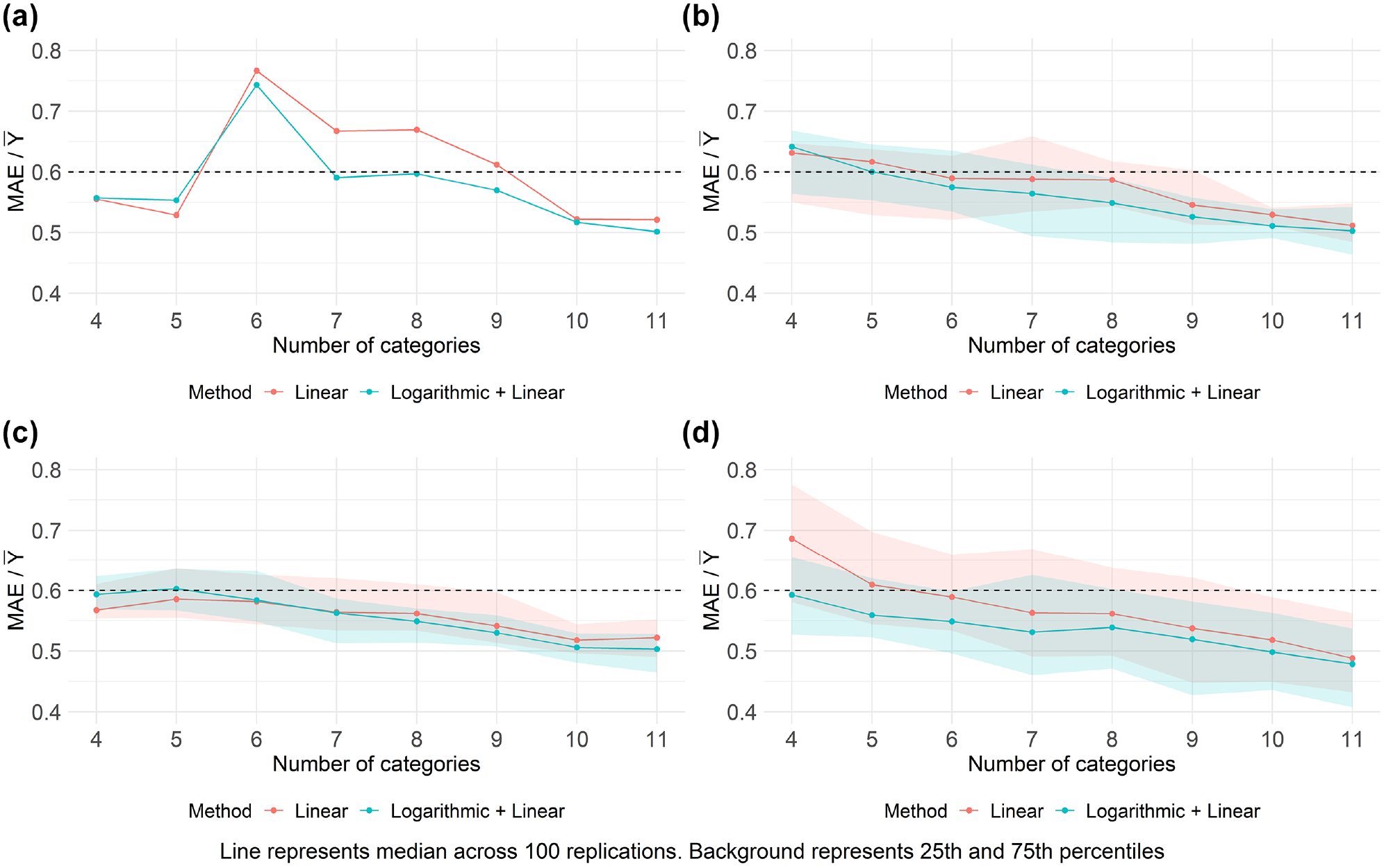
Performance assessment of original and simulated approaches: (a) original boundaries and GPT-4V ranking, (b) boundaries randomly shifted ± 1 position(s), (c) boundaries randomly shifted ± 2 position(s), and (d) simulated GPT-4V rankings.

Figure 12 presents intriguing findings. Firstly, the curves’ trends now align with expectations for the simulation approaches, showing improved performance as the number of categories increases. This supports the hypothesis that the unexpected trend observed in the original application arose from random outliers in the original GPT-4V ranking. Furthermore, the results once again demonstrate performances surpassing those of benchmark approaches, highlighting the methodology’s potential.

Secondly, notable differences in performance between the linear interpolation and logarithmic model methods were observed. While the first simulation approach yielded similar results between the methods, the second approach showed better outcomes for the logarithmic model method, especially with fewer categories. This outcome was expected considering GPT-4V’s initial misranking of the top two sites in the true ranking, placing them at positions 6 and 7. The inclusion of these sites as part of category boundaries significantly affected the performance gap between the two methods. The first simulation approach, which often excludes these sites as boundaries, resulted in comparable outcomes for linear interpolation and logarithmic model methods.

Lastly, the linear interpolation and logarithmic model methods tend to converge as the number of categories increases (Figure 12d). This convergence was expected for two reasons: (1) assuming linear interpolation adversely affects the overall performance when the first category is wider and top-ranked sites are included in the first boundary, and (2) with more categories, the two methods becomes more similar in application, since the logarithmic model is solely applied to the first category.

Conclusions and Practical Application

This work explored the use of GPT-4V as a tool to aid jurisdictions in assessing pedestrian activity within their intersections. It involved several key steps, including an initial assessment of GPT-4V’s capabilities in interpreting satellite images, the development of a method to rank sites based on pedestrian activity using GPT-4V and satellite images, and the creation of a method to estimate pedestrian volume from the GPT-4V ranking.

The initial evaluation of GPT-4V revealed its potential in interpreting satellite images, particularly in identifying different types of land use and estimating their shares within the image. Additionally, GPT-4V demonstrated its ability to rank sites based on pedestrian activity using satellite imagery.

A method utilizing GPT-4V and satellite imagery to rank intersections was proposed and applied to 48 sites within the Region of Waterloo, ON, Canada. The method yielded promising results, including a linear correlation of 0.728 between GPT-4V ranking and true ranking. Additionally, it demonstrated strong accuracy in identifying intersections with high pedestrian activity, with seven out of the top 10 sites in the true ranking appearing within the top 10 positions estimated by the proposed method. From a practical perspective, these findings underscore the potential of GPT-4V in identifying intersections with high pedestrian activity, which could help with site selection for implementing pedestrian-centric interventions.

The use of GPT-4V for ranking purposes is not without limitations. Apart from the restrictions on inputting a maximum of 10 images per query (which was further reduced to six in this work) and conducting 30 inquiries within a 3 h period, inconsistent and biased responses were observed. GPT-4V provided different responses (i.e., rankings) for the same image datasets. More significantly, we observed that 26 of the 120 rankings generated by GPT-4V may be associated with some level of bias toward the order in which the images were presented. Despite investigation, the reasons for this bias could not be identified. However, it was observed that these biased responses were not triggered by specific sites and appeared to occur randomly. This randomness somewhat mitigated the impact on ranking generation, as it introduced a degree of random error that is diluted across the rounds of simulation.

In possession of the GPT-4V ranking, a method combining the ranking and the collection of field pedestrian volume in key intersections was proposed to estimate the actual pedestrian volume for the sites in the ranking. Again, very promising results were attained, with the performance being similar to (and sometimes better than) the existing conventional approaches that are typically used to estimate pedestrian volumes in sites that lack pedestrian data information, such as the development of DD models.

The greatest benefit of the GPT-4V method is its simplicity. Unlike the development of DD models, it does not require dozens of sites with available volume data. Comparable results were obtained using five categories, which would necessitate data collection at only six sites (12.5% of the entire dataset). Furthermore, it does not require land-use, socioeconomic, or transportation GIS databases nor the development of complex statistical models. Instead, it relies on extracting satellite images, interacting with GPT-4V, and applying the relatively simple methods proposed in this work.

For future work, it is suggested that (1) the method should be applied to larger datasets to investigate whether its performance is dictated by the number or the fraction of sites used for category boundaries; (2) the method should be applied to other jurisdictions to validate its potential; (3) different zoom levels and types of satellite images (including 3D images) to develop the GPT-4V ranking should be explored and compared; (4) other types of pedestrian volume data should be employed to represent the category boundaries, specifically counts with shorter durations than the monthly average used in the present work; (5) alternative LLMs besides GPT-4V for satellite image interpretation and ranking generation should be explored; (6) GPT-4V’s capability to identify traffic volume variations both between days (e.g., weekdays versus weekends) and within a day (e.g., peak hours) based on satellite imagery should be examined; (7) the potential to enhance GPT-4V’s performance in ranking the sites by including additional information directly on the satellite image (such as the number of transit stops, commercial establishments, and so on) within a given radius of the intersection should be assessed; and (8) GPT-4V’s performance in visually identifying transportation-related elements from satellite images, such as transit stops or schools, that are important for explaining pedestrian activity should be evaluated using metrics like visual question answering.

Footnotes

Acknowledgements

The authors gratefully acknowledge (i) the Region of Waterloo for providing permission to use the pedestrian volume data and (ii) Miovision for providing access to the pedestrian data.

Author Contributions

The authors confirm contribution to the paper as follows: study conception and design: L. T. P. Sobreira, B. Hellinga; data collection: L. T. P. Sobreira, B. Hellinga; analysis and interpretation of results: L. T. P. Sobreira, B. Hellinga; draft manuscript preparation: L. T. P. Sobreira, B. Hellinga. All authors reviewed the results and approved the final version of the manuscript.

Declaration of Conflicting Interests

The author(s) declared no potential conflicts of interest with respect to the research, authorship, and/or publication of this article.

Funding

The author(s) disclosed receipt of the following financial support for the research, authorship, and/or publication of this article: The authors gratefully acknowledge financial support from the Natural Sciences and Engineering Research Council of Canada (NSERC) via the Discovery Grant Program (funding reference number 2022-03275).

ORCID iDs

Lucas Tito Pereira Sobreira

Bruce Hellinga

The work in this paper reflects the views of the authors and there is no explicit or implicit endorsement by any of the aforementioned jurisdictions/companies. The research was carried out by the authors and no endorsement of the methods or findings by funding agencies is claimed or implied.

References

AASHTO. Highway Safety Manual. American Association of Highway and Transportation Officials, Washington, D.C., 2010.

Stipancic

Miranda-Moreno

Strauss

Labbe

Pedestrian Safety at Signalized Intersections: Modelling Spatial Effects of Exposure, Geometry and Signalization on a Large Urban Network. Accident Analysis and Prevention, Vol. 134, 2020, p. 105265. https://doi.org/10.1016/j.aap.2019.105265.

Islam

Mekker

Singleton

P. A.

Examining Pedestrian Crash Frequency, Severity, and Safety in Numbers Using Pedestrian Exposure from Utah Traffic Signal Data. Journal of Transportation Engineering, Part A: Systems, Vol. 148, No. 10, 2022. https://doi.org/10.1061/jtepbs.0000737.

Munira

Sener

I. N.

Dai

A Bayesian Spatial Poisson-Lognormal Model to Examine Pedestrian Crash Severity at Signalized Intersections. Accident Analysis and Prevention, Vol. 144, 2020, p. 105679. https://doi.org/10.1016/j.aap.2020.105679.

Abohassan

El-Basyouny

Kwon

T. J.

Exploring the Associations Between Winter Maintenance Operations, Weather Variables, Surface Condition, and Road Safety: A Path Analysis Approach. Accident Analysis and Prevention, Vol. 163, 2021, p. 106448. https://doi.org/10.1016/j.aap.2021.106448.

Shinoda

Pedestrian Activity Model for prioritizing investment-A case study of sidewalk snow clearing in the City of Waterloo. Master thesis. University of Waterloo, Ontario, Canada, 2018.

Orr

Estimating Average Annual Daily Pedestrian Volumes at Intersections based on Turning Movement Counts. Master thesis. University of Waterloo, Ontario, Canada, 2021.

Johnstone

Nordback

Kothuri

Annual Average Nonmotorized Traffic Estimates from Manual Counts: Quantifying Error. Transportation Research Record: Journal of the Transportation Research Board, 2018. 2672: 134–144.

Nordback

Johnstone

Kothuri

Optimizing Short Duration Bicycle and Pedestrian Counting in Washington State. Research Report WA-RD 875.2. Washington State Department of Transportation, Olympia, 2017.

10.

Singleton

P. A.

Park

Lee

D. H.

Varying Influences of the Built Environment on Daily and Hourly Pedestrian Crossing Volumes at Signalized Intersections Estimated from Traffic Signal Controller Event Data. Journal of Transport Geography, Vol. 93, 2021, p. 103067. https://doi.org/10.1016/j.jtrangeo.2021.103067.

11.

Schneider

R. J.

Schmitz

Qin

Development and Validation of a Seven-County Regional Pedestrian Volume Model. Transportation Research Record: Journal of the Transportation Research Board, 2021. 2675: 352–368.

12.

Griswold

J. B.

Medury

Schneider

R. J.

Amos

Grembek

A Pedestrian Exposure Model for the California State Highway System. Transportation Research Record: Journal of the Transportation Research Board, 2019. 2673: 941–950.

13.

Sanders

R. L.

Frackelton

Gardner

Schneider

Hintze

Ballpark Method for Estimating Pedestrian and Bicyclist Exposure in Seattle, Washington: Potential Option for Resource-Constrained Cities in an Age of Big Data. Transportation Research Record: Journal of the Transportation Research Board, 2017. 2605: 32–44.

14.

Hankey

Mondschein

Buehler

Spatial Models of Active Travel in Small Communities: Merging the Goals of Traffic Monitoring and Direct-Demand Modeling. Journal of Transport & Health, Vol. 7, 2017, p. 149–159. https://doi.org/10.1016/j.jth.2017.08.009

15.

Sobreira

L. T. P.

Hellinga

Comparing Direct Demand Models for Estimating Pedestrian Volumes at Intersections and Their Spatial Transferability to Other Jurisdictions. Transportation Research Record: Journal of the Transportation Research Board, 2023. 2677: 260–271.

16.

Sobreira

L. T. P.

Hellinga

Enhancing the Spatial Transferability of Direct Demand Models for Estimating Pedestrian Volumes at Intersections. Transportation Research Record: Journal of the Transportation Research Board, 2024. 2678: 245–260.

17.

Sobreira

L. T. P.

Hellinga

Expanding Short-Term Pedestrian Volume Counts to Average Annual Daily Counts at Intersections: Temporal Pattern Indices and a Comparison of Statistical Land Use and Simple Threshold Methods. Transportation Research Record: Journal of the Transportation Research Board, 2024. https://doi.org/10.1177/03611981241281736.

18.

Humagain

Singleton

P. A.

Advances in Pedestrian Travel Monitoring: Temporal Patterns and Spatial Characteristics using Pedestrian Push-Button Data from Utah Traffic Signals. Journal of Transport and Land Use, Vol. 14, No. 1, 2021, pp. 1341–1360. https://doi.org/10.5198/jtlu.2021.2112.

19.

Medury

Griswold

J. B.

Huang

Grembek

Pedestrian Count Expansion Methods: Bridging the Gap between Land Use Groups and Empirical Clusters. Transportation Research Record: Journal of the Transportation Research Board, 2019. 2673: 720–730.

20.

Nordback

Kothuri

Johnstone

Lindsey

Ryan

Raw

Minimizing Annual Average Daily Nonmotorized Traffic Estimation Errors: How Many Counters Are Needed per Factor Group?

Transportation Research Record: Journal of the Transportation Research Board, 2019. 2673: 295–310.

21.

Grossman

Rodgers

M. O.

Guensler

Watkins

If Safety Matters, Let’s Measure It: Nationwide Survey Results for Bicycle and Pedestrian Treatment Prioritization. Journal of Transportation Engineering, Part A: Systems, Vol. 145, No. 1, 2019. https://doi.org/10.1061/JTEPBS.000020.

22.

Singleton

P. A.

Runa

Pedestrian Traffic Signal Data Accurately Estimates Pedestrian Crossing Volumes. Transportation Research Record: Journal of the Transportation Research Board, 2021. 2675: 429–440.

23.

Lian

Loo

B. P. Y.

Fan

Advances in Estimating Pedestrian Measures Through Artificial Intelligence: From Data Sources, Computer Vision, Video Analytics to the Prediction of Crash Frequency. Computers, Environment and Urban Systems, Vol. 107, 2024, p. 102057. https://doi.org/10.1016/j.compenvurbsys.2023.102057.

24.

Hankey

Zhang

H. T. K.

Hystad

James

Predicting Bicycling and Walking Traffic Using Street View Imagery and Destination Data. Transportation Research Part D: Transport and Environment, Vol. 90, 2021, p. 102651. https://doi.org/10.1016/j.trd.2020.102651.

25.

Chen

Sheng

Wang

Liu

Estimating Pedestrian Volume Using Street View Images: A Large-Scale Validation Test. Computers, Environment and Urban Systems, Vol. 81, 2020, p. 101481. https://doi.org/10.1016/j.compenvurbsys.2020.101481

26.

Open AI. ChatGPT-4 Vision. 2024. https://chatgpt.com/

27.

Driessen

Dodou

Bazilinskyy

De Winter

Putting ChatGPT Vision (GPT-4V) to the Test: Risk Perception in Traffic Images. Preprint, 2023. https://www.researchgate.net/publication/375238184.

28.

Huang

Jiang

Gautam

Saripalli

GPT-4V Takes the Wheel: Promises and Challenges for Pedestrian Behavior Prediction. arXiv, 2024. https://doi.org/10.48550/arXiv.2311.14786

29.

Google Maps. Set of Images Showing Aerial Views from Different Intersection in the Region of Waterloo, Canada [Google Maps images]. January 2024 using the package httr from R. 2024. https://maps.googleapis.com/maps/api/staticmap.

30.

Google. Google Maps Static API. https://developers.google.com/maps/documentation/maps-static/start. Accessed January 2024.

31.

Wickham

httr: Tools for Working with URLs and HTTP. R package version 1.4.4. 2022. https://CRAN.R-project.org/package=httr. Accessed January 2024.

32.

Schulhoff

Ilie

Balepur

Kahadze

Liu

, et al. The Prompt Report: A Systematic Survey of Prompting Techniques. arXiv, 2024. https://doi.org/10.48550/arXiv.2406.06608

33.

StreetLight. StreetLight Pedestrian Volume Methodology and Validation White Paper. 2023. https://learn.streetlightdata.com/pedestrian-methodology-validation. Accessed April 2024.

Estimating Pedestrian Volumes at Intersections using Artificial Intelligence: A ChatGPT Vision Approach

Abstract

Keywords

Framework

Datasets

CAN GPT-4V Visually Assess Satellite Images?

Ranking Intersections: GPT-4V and Satellite Images

Method

Results

Exploring GPT-4V Responses

Inconsistencies in GPT-4V Responses

Exploring Potential Bias in GPT-4V Responses

Estimating Pedestrian Volume From Rankings

Method

Results

Simulation Approaches

Conclusions and Practical Application

Footnotes

Acknowledgements

Author Contributions

Declaration of Conflicting Interests

Funding

ORCID iDs

References