
Abstract
The integrated Transport Land-use and Energy (iTLE) model is combined with traffic and emission simulators to examine the effects of electric vehicle (EV) adoption on traffic networks and greenhouse gas (GHG) emissions reduction. The research uses data from the 2022 Halifax Travel Activity (HaliTRAC) survey to develop an EV type choice model within iTLE, while traffic and emission simulators are created on PTV VISUM and MOVES3.0 platforms. Along with the base case scenario (2022), two more scenarios are considered at five-year intervals: 2027 (scenario-1), and 2032 (scenario-2). The traffic assignment model is calibrated and validated for the base year (2022) considering traffic volume data of fifty (50) different intersections of Halifax Regional Municipality (HRM). The findings reveal that the younger generation, higher-income households, and full-time workers are more inclined to adopt EVs in the future. The estimated EV adoption rate for 2027 is 16.3% from the base year (2022), increasing to 31% by 2032. Regarding GHG emissions, the morning peak period in 2027 witnessed a notable 18.5% decrease compared to the base year of 2022, and in 2032, this reduction became even more substantial at 31.8% compared to 2027. Similarly, the evening peak period also experienced significant declines, with a 22.4% decrease in 2027 and a more remarkable 32.9% reduction in 2032. The outcomes of this research will be valuable for urban planners, engineers, and government officials when implementing climate action plans as they devise effective policy measures related to vehicles.
Keywords
Over the past few decades, the increasing urgency of climate change has amplified the global demand for a large-scale transition to sustainable transportation alternatives. The adoption of electric vehicles (EVs) is a significant component of clean energy initiatives, contributing to the establishment of a sustainable transportation network. Governments and public authorities worldwide have been consistently working toward implementing various policies aimed at enhancing the market presence of EVs and decreasing greenhouse gas (GHG) emissions caused by the transportation sector.
To avert the worst impacts of climate change, the Government of Canada is committed to achieving net-zero emissions by 2050 ( 1 ). The 2030 Emissions Reduction Plan (ERP) is an ambitious but achievable roadmap that outlines a sector-by-sector course of actions for Canada to reach its emissions reduction target of 40% below 2005 levels by 2030 and net-zero emissions by 2050 ( 2 ). In 2016, the transportation sector represented approximately 20% of community emissions in the Halifax Regional Municipality (HRM), with 90% represented by light duty, personal vehicles. To reflect Canada’s net-zero climate action plan, the HRM developed and approved the HalifACT action plan in June 2020. The HalifACT action plan provides long-term guidance to reduce emissions and help communities adapt to a changing climate. While the HalifACT action plan first recommends a transition to public transit or active transportation, it also recommends that the municipality take significant action to accelerate the transition to EVs. Even though EVs may not directly address concerns related to automobile dependency, urban sprawl, or traffic congestion, they still play a role in improving air quality and mitigating GHG emissions. The 2022 Halifax Travel Activity (HaliTRAC) survey was conducted in the HRM region to collect people’s household characteristics, the individual characteristics of household members, their 24-h travel log, and their travel behaviors, including the likelihood they will adopt an EV within the next five years.
Therefore, a comprehensive modeling framework that acknowledges multiple scenarios in the HRM is developed in this study to examine the impact of EVs on roadway traffic operations and vehicular emissions. This research builds on an integration between activity-based travel demand forecasting models and traffic flow and emission simulators. To achieve these goals, this study has three primary objectives: (1) develop a micro-behavioral EV adoption model within an activity-based modeling framework; (2) analyze the impact of EVs on the traffic network; and (3) estimate the GHG emission reduction of the traffic network. The EV adoption model is developed following random utility-based econometric modeling techniques and a mixed logit (MXL) model, and implemented with an integrated transport land use and energy (iTLE) model that follows the activity-based travel forecasting approach. The iTLE model has been validated for multiple years with Canadian census data and HaliTRAC survey data. In a nutshell, the proposed tool can accommodate EV adoption along with its impact on traffic operations and network emissions. The findings from this research will assist planners, engineers, and government officials to administer effective policy interventions related to vehicle electrification, which will improve traffic operations and the decision-making processes outlined in climate action plans.
Literature Review
Sustainable transportation systems require a significant reduction in GHG emissions and air pollution control, and a decreased dependence on fossil fuels. To achieve these targets, vehicle electrification along with analyzing its effectiveness on the traffic network are necessary. The literature review of this study is divided into two parts: (1) the development of an EV adoption model and (2) the integration of an activity-based travel demand model with traffic assignment and emission simulators to evaluate traffic operations and vehicular emissions.
Adoption of Electric Vehicles
The adoption of EVs relies significantly on explicit external factors, such as emissions regulations, increasing gasoline prices, financial incentives, limited awareness, low consumer risk tolerance, and high initial production costs ( 3 – 5 ). In recent years, substantial research has been carried out to understand the factors that influence the adoption of EVs the most. A study by Axsen et al. ( 6 ) revealed that consumers prioritize long driving ranges and fast charging times as factors of concern when considering the adoption of an EV. On the other hand, the perceived benefits of EVs, such as lower operating costs and reduced environmental impact, have a positive influence on consumer attitudes. The adoption of EVs is greatly influenced by government policies and incentives. Financial incentives, including subsidies and tax credits, play a critical role in stimulating EV adoption. In addition, policy measures, such as zero-emission vehicle mandates and low-emission zones, have been proven to increase EV sales ( 7 ). Adequately developed and easily accessible charging infrastructure is vital to reduce anxiety around the driving range and foster the adoption of EVs. Consumers frequently weigh up the availability of public charging stations when making decisions about adopting EVs ( 8 ). Moreover, strategically placing charging stations in residential areas, workplaces, and public spaces has been shown to further encourage EV uptake. Canadians who observed a charging station in their community displayed 9% more interest in EVs compared to their counterparts ( 9 ). The integration of an EV into one’s lifestyle may serve as a symbol of individuality and social status. For instance, according to a study conducted by Schuitema et al. ( 10 ) in the United Kingdom (UK), adopting an EV can be motivated by a desire to showcase a distinct self-identity and generate a sense of pride. In addition, demographic factors, such as age and gender, also influence EV adoption. Socioeconomic characteristics, including income, education level, and urban/rural residence, are significant determinants ( 8 ). Advancements in EV technology, such as improvements in battery capacity and reductions in manufacturing costs, are instrumental to EV adoption. As EV technology evolves, consumers become more attracted to the improved performance and cost-effectiveness of EVs ( 11 ). Lastly, environmental awareness and climate change concern play a crucial role in consumers’ decisions to adopt EVs. Consumers with strong environmental values are more inclined to consider EVs as a sustainable transportation option ( 12 ). There has been limited research that examined factors affecting EV choices and integration of the behavioral model instead of the data-driven model within an activity-based travel demand forecasting simulation platform. This study comprehensively incorporates a behavioral model within the operational modeling framework using a large-scale survey data for the HRM.
Integrated Land Use, Transportation, and Emission Models
Over the past 40 years, significant advancements have been achieved in travel demand modeling. Transportation models have evolved from macroscopic approaches to highly granular behavioral activity-based models. In addition, most models transitioned from generating aggregate zonal level estimations to employing disaggregated agent-based models ( 13 ). In the past, conventional transportation models tended to examine aspects of the transportation system, such as travel demands, traffic flows, and emissions, in isolation from one another. Efforts to connect these distinct models into a cohesive and unified system were undertaken by the transportation community when the importance of integrating these phenomena was realized ( 14 ). Most activity-based models do not include built-in traffic flow and emission simulators. Several projects, such as SimMobility ( 15 ) and POLARIS ( 14 , 16 ) sought to develop integrated travel demand models with dynamic traffic assignment procedures. Several researchers have succeeded in coupling land use and travel behavior models with existing dynamic traffic assignment software, such as MATSim and EMME/2. Abou-Senna et al. ( 17 ) investigated four different approaches to capture the environmental impacts of vehicular operation on a limited access highway in Orlando, Florida. They calculated the emission considering the average traffic volume and vehicular speed and also advanced the model addressing an integration between the VISSIM and MOtor Vehicle Emission Simulator (MOVES) platforms, named VIMIS. Moreover, Alam et al. ( 18 ) also developed a connection between traffic simulation and the MOVES model to explore the impact of traffic emission and air quality in densely populated urban areas in the City of Montreal, Canada. They examined multiple scenarios, such as fleet renewal, street closures, and the reduced traffic situation, within this integrated modeling framework. This study demonstrates the importance of analysis of air quality as an additional dimension to the evaluation of traffic management plans and their effects on network emissions. Xie et al. ( 19 ) integrated the MOVES platform and the PARAMICS microscopic traffic simulation tool to evaluate the environmental impacts of three alternative transportation fuels—electricity, ethanol, and compressed natural gas. They also estimated the daily fuel savings and emission reduction of alternative fueled vehicles on the road network. Gu et al. ( 20 ) examined whether the change of construction working shift from daytime to nighttime can be beneficial to improve air quality. They investigated the impact of vehicular emissions by making a coupling between traffic simulation and the Environmental Protection Agency’s (EPA’s) MOVES emission simulator. They utilized the link-based method and operating mode-based method. Not only calculating emissions, MOVES software was utilized to explore the sensitivity between vehicular speed and emission rate. Wu et al. ( 21 ) explored that emission rates are higher for the speed range 25–50 mph in Beijing, China, than any other speed interval with the same type of vehicle characteristics. Briema et al. ( 13 ) integrated mobiTopp, an agent-based travel demand model, and MATSim, a dynamic traffic assignment model, to create a travel demand model. Ziemke et al. ( 22 ) integrated CEMDAP and MATSim models to assess the capacity to transfer transport demand models. Another study integrated a land use model, SILO (simple integrated land use orchestrator), a land cover model, CBLCM (Chesapeake Bay land change model), an advanced trip-based model, MSTM (Maryland statewide transportation model), and emission models, the MEM (mobile emissions mode) and BEM (building energy-consumption and emissions model), in different environments using Python wrappers ( 23 ). ArcGIS Model Builder was then used to provide a graphical user interface and to present the models’ workflow. Moeckel et al. ( 24 ) integrated an economic model, a land use model, a travel demand model, and an environmental model for the Chesapeake Bay Mega region.
Expanding on the approaches described above, this study aims to integrate an activity-based model of the iTLE model with traffic flow and emission simulators. The paper advances a tool coupling approach for integration and adds a new EV adoption model for traffic flow and emission estimation. This work contributes to the literature in three ways, as follows: (1) incorporating an EV module within an iTLE model; (2) adopting a dynamic traffic flow simulator (TFS) model coupled with the iTLE process; and (3) integrating an emission simulator within the EPA’s MOVES platform to estimate the GHG emissions for different scenarios in the HRM.
Data Source
Primary and Secondary Data
The 2022 HaliTRAC survey data, the first large-scale random sample survey conducted in the HRM region, is used primarily in this study. The survey was conducted in four phases. A total of 3731 households, including 5095 household members, completed their survey with a completion rate of 13.6%. The study area is shown in Figure 1.
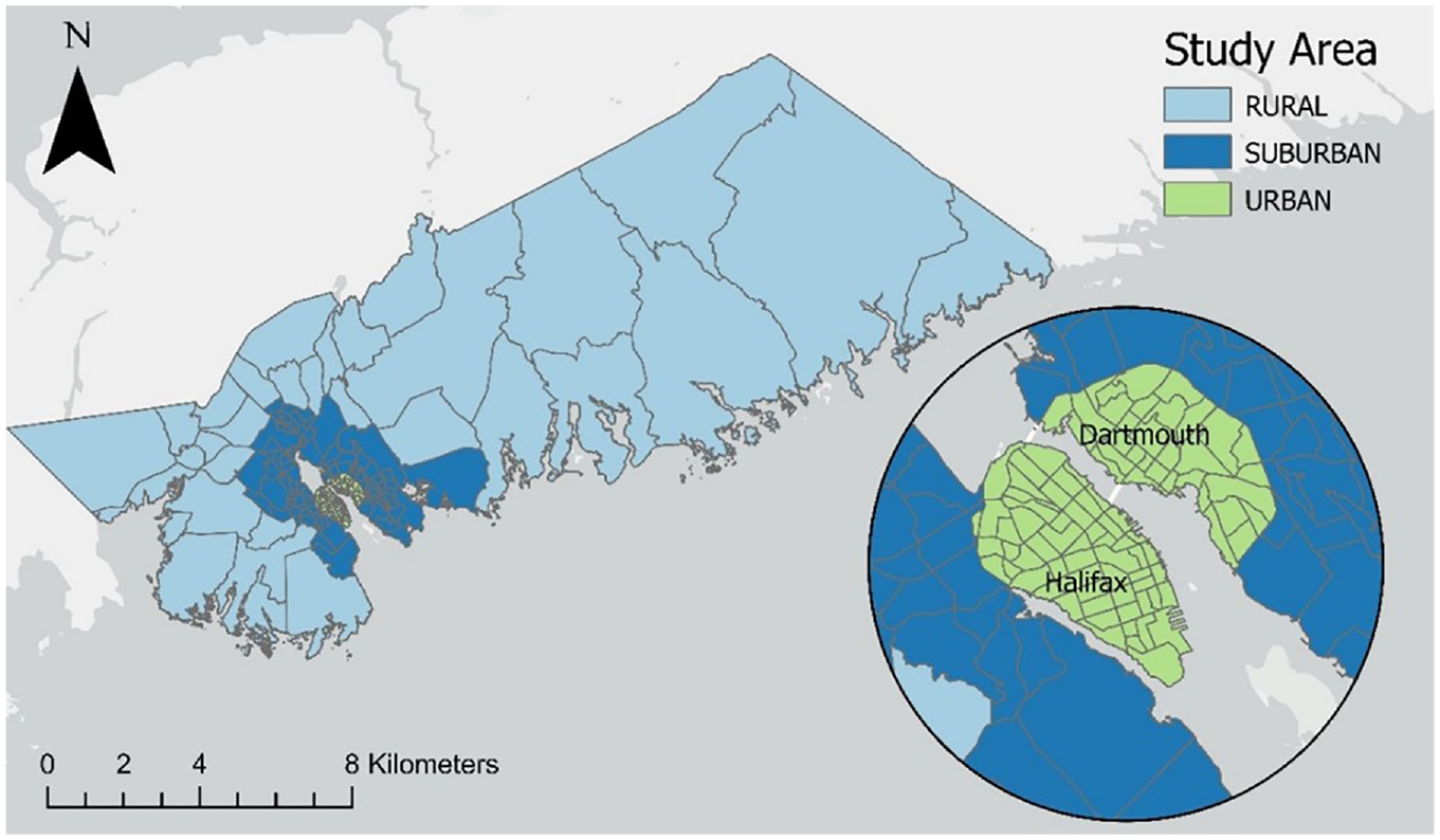
Study area—Halifax Regional Municipality (HRM).
The survey collected information on three central themes: household characteristics, individual attributes, and a 24-h travel log for each member of the household. Firstly, respondents were asked to provide information about their household and each member in the household. After that, each member was asked to record their travel activities for a 20-h period of a typical weekday. Moreover, the survey included multiple attitudinal and preference-related questions to understand the respondents’ perceptions of shared travel, working from home, EV adoption, and so on. For additional analysis, neighborhood characteristics and accessibility measurements were considered within the modeling framework. These datasets were collected from 2021 Canadian Census data at the dissemination level and the HRM open data portal. Neighborhood characteristics included the data related to dwelling and population density at the dissemination level. Accessibility measurements incorporated household members’ distance from their home to the nearest central business district (CBD), shopping mall, recreation park, bus stop, and much more. All these distances were measured after geocoding the location of every household using ArcGIS Pro software.
Data Description
During the parameter estimation of the EV adoption model, many variables are considered and classified into four categories, including individual characteristics, household characteristics, accessibility, and neighborhood characteristics. Individual characteristics incorporate information related to household members’ age, gender, employment status, and education level. Household characteristics consider homeownership status, annual household income, and current vehicle information. In addition, the distance from the household to the nearest CBD and shopping mall, as well as dwelling density, are incorporated into the modeling framework. According to the survey results, more than 55% of respondents were less than 60 years old. Males and females almost shared equal proportions. Approximately 45% of individuals were working full-time. Similarly, household characteristics showed that most survey respondents owned a house (with a total of 78.26%) and more than 45% of households had an annual income over C$100,000. With respect to accessibility and neighborhood characteristics, the average household to the nearest CBD distance was 6.655 km with a standard deviation of 9.082, the average household to their school distance was 1.067 km with a standard deviation of 1.431, the average household to the nearest shopping mall distance was 4.827 km with a standard deviation of 8.260, the average household to the nearest recreational park distance was 0.281 km with a standard deviation of 0.592, and the average dwelling density was 2396 with a standard deviation of 378. Descriptive statistics of the model data are presented in Table 1.
Descriptive Statistics of Explanatory Variable(s)
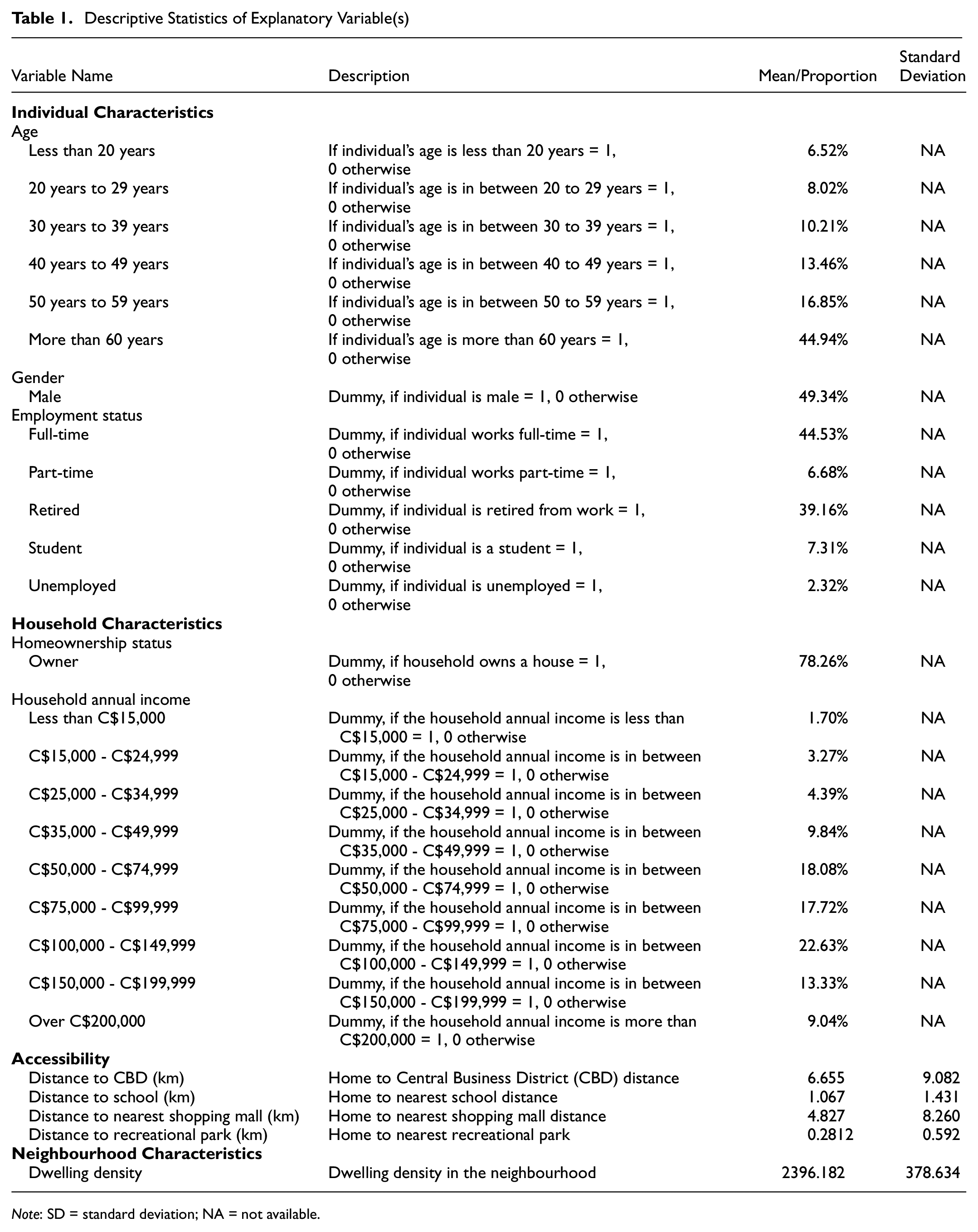
Note: SD = standard deviation; NA = not available.
Methodology
The methodology of this research can be classified into three phases: (1) update the vehicle type choice model in an activity-based travel demand forecasting model of the iTLE to incorporate the adoption of different types of EVs, such as battery electric vehicles (BEVs), plug-in hybrid electric vehicles (PHEVs), and hybrid electric vehicles (HEVs); (2) address the dynamic traffic assignment model in the VISUM platform to analyze different traffic operation scenarios with EVs; and (3) develop a county-level emission estimation process within the EPA’s MOVES. The study incorporated a tool coupling approach to couple the iTLE simulator with the traffic assignment procedure of PTV VISUM and the emission estimation process of the EPA’s MOVES platform. The conceptual framework of this study is addressed in Figure 2.
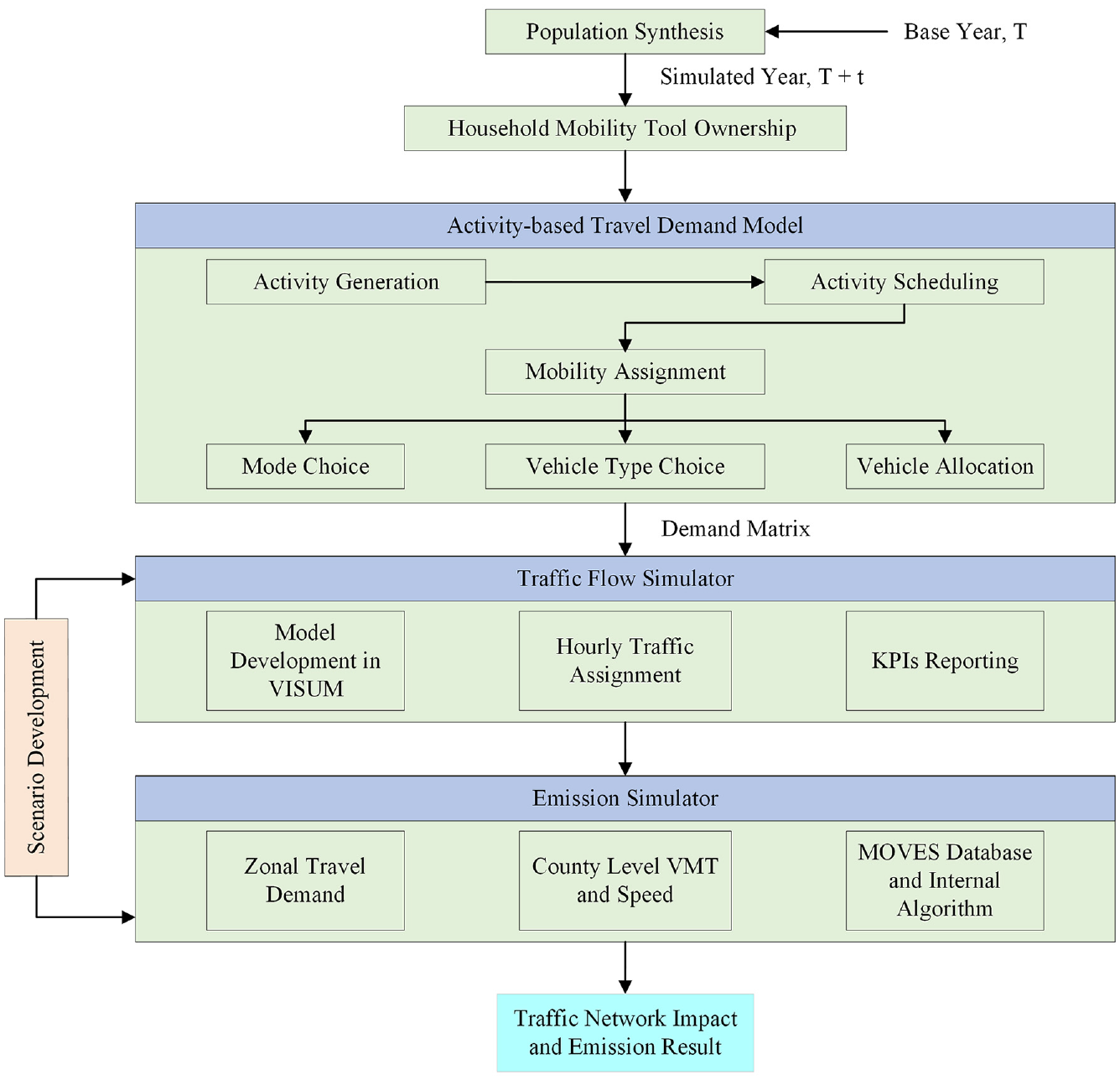
Conceptual framework of integrated activity-based travel demand, traffic flow, and emission models.
Activity-Based Travel Demand Forecasting Model
The integrated iTLE model consists of multiple modular-based systems, so that each module and micro-behavioral model within the said module can be updated or modified without affecting the whole microsimulation process. At present, the iTLE simulation platform is implemented using the C# programming language under the .NET platform ( 25 ). The simulation process begins with population synthesis, which has three core components: (1) a longer-term decision simulator (LDS); 2) a shorter-term decision simulator (SDS); and 3) a TFS. The LDS module includes information related to the life-stage transition, residential location, and different types of mobility tool ownership. A detailed description of LDS model development is found in Fatmi and Habib ( 26 , 27 ). The SDS consists of three major segments: activity generation, activity scheduling, and mobility assignment. The microsimulation process of SDS begins with simulating individuals’ daily activities. After the generation of activity, the activity scheduling sub-module starts simulating individuals’ schedules. The activity scheduling sub-module has three steps, including agenda formulation, destination choice, and shared travel choice. The final microsimulation process of SDS is mobility assignment, which consists of mode choice decisions and a vehicle allocation model. Detailed descriptions of the SDS microsimulation modeling framework can be found in Khan and Habib ( 28 , 29 ). This research enhances the mobility assignment component of SDS by incorporating the vehicle type choice mel. The vehicle type choice model offers the opportunity to choose regular gasoline or diesel-driven vehicles and different types of EVs for those who have vehicle ownership. If an individual does not have ownership of a vehicle, other types of mode, such as transit, walking, and biking, are assigned within the microsimulation framework. The model can simulate travel decisions on a year-by-year basis. This study considers the mode share decisions of 2022 as the base year (2022), Scenario 1 (2027), and Scenario 2 (2032) and does not include the infiltration of EVs. The two other scenarios are developed to address the micro-behavioral model of EV adoption using a five-year interval, comparing 2027 (scenario-1) to 2032 (scenario-2). Overall, three scenarios are considered at two peak periods (morning and evening) to analyze traffic operations and transport emissions. The conceptual framework for the enhanced mobility assignment process is shown in Figure 3.
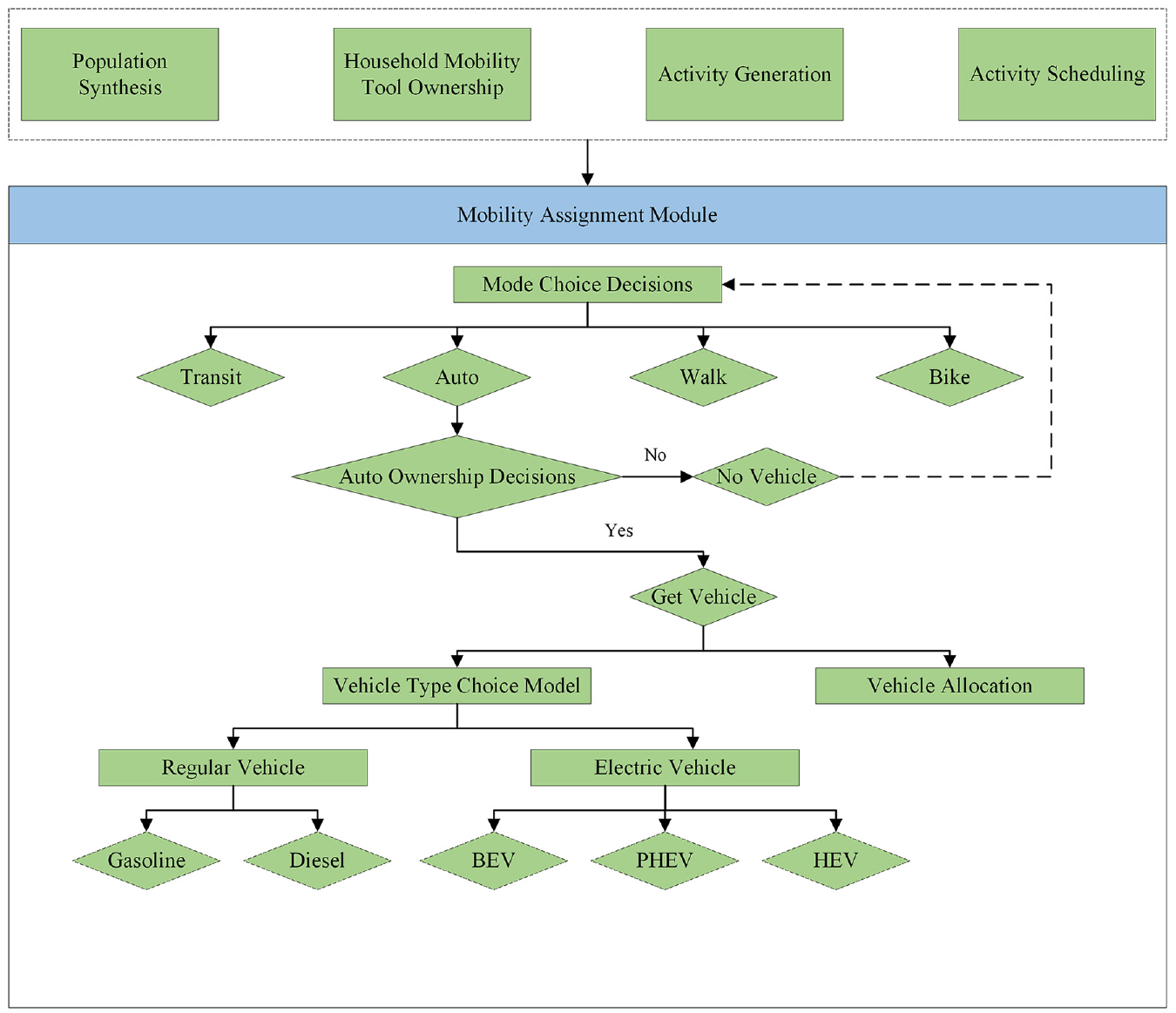
Conceptual framework for the mobility assignment process.
The vehicle type choice model is developed following the MXL econometric modeling approach. To develop the MXL model, let us assume that the utility

Here,

The equation above represents conditional probability where the choice probability is conditional on

Here,

Here,
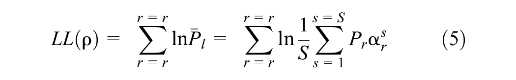
For comparison purposes, a conventional multinomial logit (MNL) model is developed as well. The results are compared, following different criteria suitability along with the log-likelihood value, such as Bayesian information criteria (BIC) or Akaike information criteria (AIC). The lower values of the AIC and BIC values indicate the optimum number of classes. AIC and BIC can be calculated using the following equation:


Here,
Traffic Assignment Model
For this study, a VISUM-based TFS model was developed for the HRM region and integrated with the prototype iTLE model. This model has two components: (1) roadway assignment (i.e., auto trips and truck movements are assigned under this procedure) and (2) public transit assignment (i.e., a timetable-based assignment of transit users on regular buses, express buses, and ferry services). The origin–destination (OD) matrices are extracted from the iTLE modeling framework as it can generate travel information, including the start time, end time, OD location, mode share, and others. This set of information is used to generate OD matrices for two peak periods, the morning peak period (7:00–9:00 a.m.) and the evening peak period (4:00–6:00 p.m.). During the formation of OD matrices, the study considers different types of auto mode shares, such as BEVs, PHEVs, HEVs, and regular vehicles (i.e., gasoline or diesel driven). The road network has four categories: expressways or highways, arterial roads, collector roads, and local roads. The study area developed in VISUM contains 219 traffic analysis zones (TAZs), of which 95 are in the urban area. The urban area has mixed land uses, including commercial, industrial, and residential uses ( 30 ). Downtown Halifax and Dartmouth fall into this category. The suburban area surrounding the urban area contains 92 TAZs, which are mostly used for residential purposes and a few for industrial and commercial uses. Finally, the suburban area is surrounded by 32 TAZs of the rural area.
Dynamic Stochastic Assignment
The proposed model can perform several static and dynamic assignment methods. The static assignment method includes an incremental assignment, a user equilibrium assignment, a stochastic assignment, and many other assignments. The user equilibrium assignment is one of the most preferred static assignment methods in transportation applications (
31
). The model’s equilibrium assignment process allocates demand in accordance with Wardrop’s first principle, which states that travelers in a transportation network select the route with the minimum perceived travel time. The proposed model can perform several dynamic assignment methods, such as the dynamic user equilibrium assignment (DUE), stochastic dynamic assignment (SDA), and simulation-based dynamic assignment (SBA). The SDA method was used in this study and stands apart from other assignment procedures because of its explicit modeling of the travel time required to complete trips within the network. First off during the assignment, the defined assignment period,
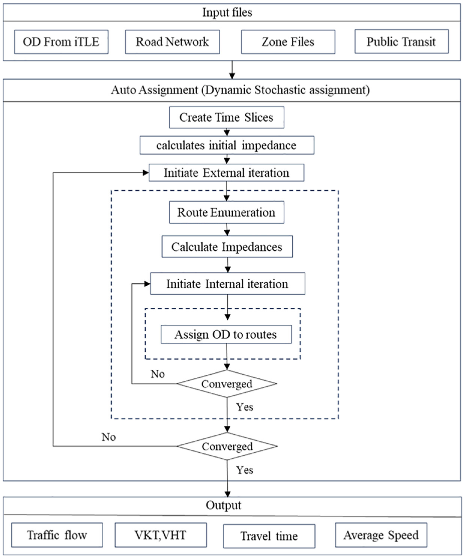
Framework for the dynamic stochastic traffic assignment model developed in VISUM.
Calibration and Validation of the Traffic Assignment Model
Model calibration and validation play a significant role in improving the credibility and forecasting capabilities. The traffic microsimulation model can analyze the 24-h network impact considering the OD matrices obtained from the iTLE model. The OD generation algorithm integrated within the iTLE model can generate hourly OD matrices for different modes, such as car, transit, walk, and bike. To generate OD matrices, information on individuals’ activity schedule, trip chain, home location, trip destination, and mode choice are utilized. This time-dependent OD matrix was validated against the HaliTRAC 2022 survey data. Figure 5 provides a framework for the model calibration and validation adopted in this study.
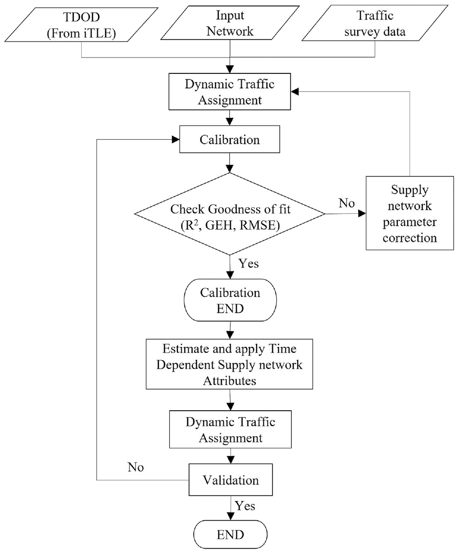
Framework for traffic assignment model calibration and validation.
The traffic assignment model used in this study was calibrated for the year 2022 for three distinct peak hours: the morning peak hour (8:00–9:00 a.m.), afternoon peak hour (noon–1:00 p.m.), and evening peak hour (4:00–5:00 p.m.). A comprehensive dataset from 50 locations, spanning two directions, was utilized during the calibration process. The supply network parameters were calibrated using a trial-and-error method to match the survey volume and the model flow. Initially, the entire network was divided into small segments, and calibration was carried out segment by segment by adjusting key link and node attributes such as capacities, speeds, volume-delay functions (VDFs), junction delays, and so forth. Finally, the overall network was considered to reach an acceptable goodness of fit. Three measures of goodness of fit were used in the calibration process: the GEH statistics (Geoffrey E. Havers statistics), root mean square error (RMSE), and R-squared (R2) ( 32 , 33 ). The GEH statistics play a pivotal role in traffic engineering, traffic forecasting, and traffic modeling, serving as a crucial instrument for comparing two sets of traffic volumes. A smaller GEH statistics value signifies reduced variance with the observed data, indicative of higher model acceptance. Similarly, the RMSE and R2 are the measures of the average magnitude of errors between predicted and observed values. Lower RMSE values and higher R2 values denote superior model performance in the realm of traffic analysis. During the calibration, GEH statistics < 5 on 85% of the locations and R2 > 0.9 were considered as the acceptable level. For validation, GEH statistics < 10 on 75% of the locations and R2 > 0.85 were considered as the acceptable level ( 32 , 34 ). Time-period-dependent network attributes are developed based on the peak hour calibrated network attributes and applied to the relevant peak period traffic assignments (i.e., for 6:00–10:00 a.m., morning peak hour calibration parameters were used; 10:00 a.m.–4:00 p.m.—afternoon, and 4:00–10:00 p.m.—evening). This approach to traffic assignment was also validated for 1 h of each peak period assignment. Figure 6 shows the calibration and validation results.
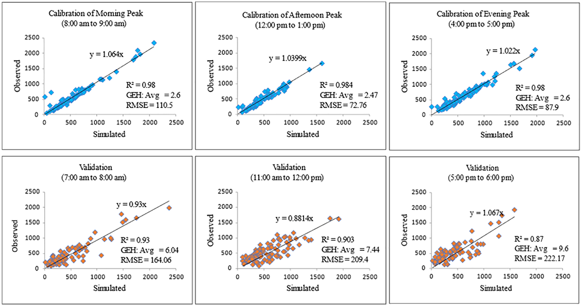
Traffic assignment model calibration and validation results.
Emission Modeling
The emission simulator for the HRM is developed in the MOVES3.0 platform and considers three scenarios for two peak periods: (i) the morning peak period (7:00–9:00 a.m.) and (ii) the evening peak period (4:00–6:00 p.m.). The model uses several inventories from multiple data sources and results from the traffic assignment model. The required different built-in data inventories, such as the source type population, vehicle type vehicle miles traveled (VMT) distribution, road type distribution, and fuel supply data, are obtained from the transport network model developed in VISUM. The emission simulator defines five different road types: (i) off-network, (ii) rural restricted access, (iii) rural unrestricted access, (iv) urban restricted access, and (v) urban unrestricted access. The ratio of these roads within the HRM is calculated using the traffic network model. In this emission simulator, only the proportion of vehicles is utilized and the MOVES platform provides an option to address the percentage of regular vehicles and EVs. One of the primary constraints of the emission simulator is that it cannot consider the emissions that occurred from the presence of PHEVs and HEVs in the network. Therefore, the PHEVs and HEVs were converted to equivalent to regular vehicles by applying conversion factors calculated based on the amount of GHG emissions they produce compared to regular vehicles. On average, HEVs emit 0.55 times the emissions of a regular gasoline vehicle and PHEVs emit 0.23 times the emissions of a regular gasoline vehicle ( 35 ). Vehicle age distribution and meteorology data are collected from a variety of available sources. Hourly meteorological data is from the Halifax Naval Dockyard weather station for the year 2022 obtained through Environment Canada ( 36 ). In addition, default data extracted from MOVES software is used for average speed distribution and inspection and maintenance (I/M) programs. Multiple iterations are executed within the emission simulator during GHG emission estimation. After the execution is completed, a summary report for emissions is generated in the post-processing step, which provides the emissions from all source types. In this study, only the GHG emissions that are CO2 equivalents are considered. A detailed framework is given in Figure 7.
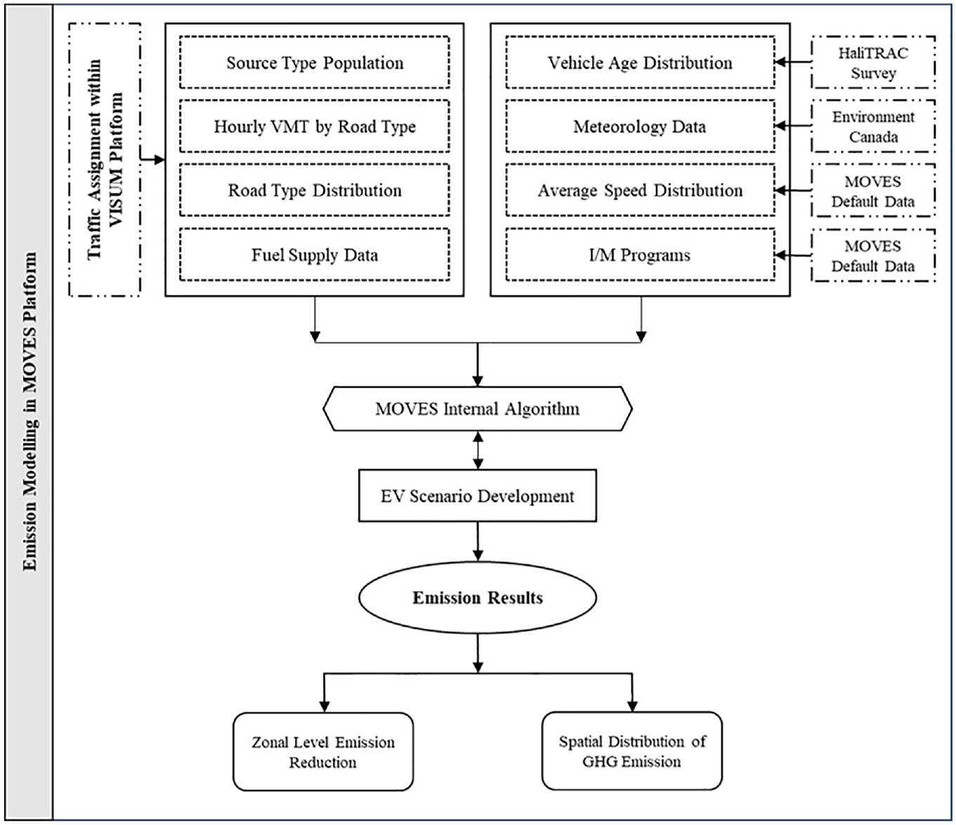
Framework for the emission simulator developed in the MOtor Vehicle Emission Simulator (MOVES).
Results and Discussion
The results section of this study is divided into three parts. Firstly, it explains the EV type choice model developed through a random utility-based econometric modeling approach. Next, it analyzes the traffic network impact from the incorporation of EVs in household vehicle ownership. To make a comparison among different scenarios of EV adoption, this research uses the TFS software coupled with the iTLE model. Finally, the proportion of emission reduction generated through the emission simulator is mentioned following different scenarios. A brief description of the model results is given below.
EV Type Choice Model Result
This research considers both the MNL and MXL econometric modeling approaches, although the MXL model outperforms the MNL model’s result following different goodness of fit criteria, such as the log-likelihood, AIC, BIC, and R2 value. In addition, the MXL model has the ability to capture unobserved heterogeneity in the survey responses, which may have a potential impact on the decision-making process. The MXL model allows for more flexible distributional assumptions for the random parameters than the MNL model. This flexibility enables the model to capture a wider range of preference distributions and accommodate complex choice behavior. The model results can be found in Table 2.
Parameter Estimation Results for Electric Vehicle Type Choice Model
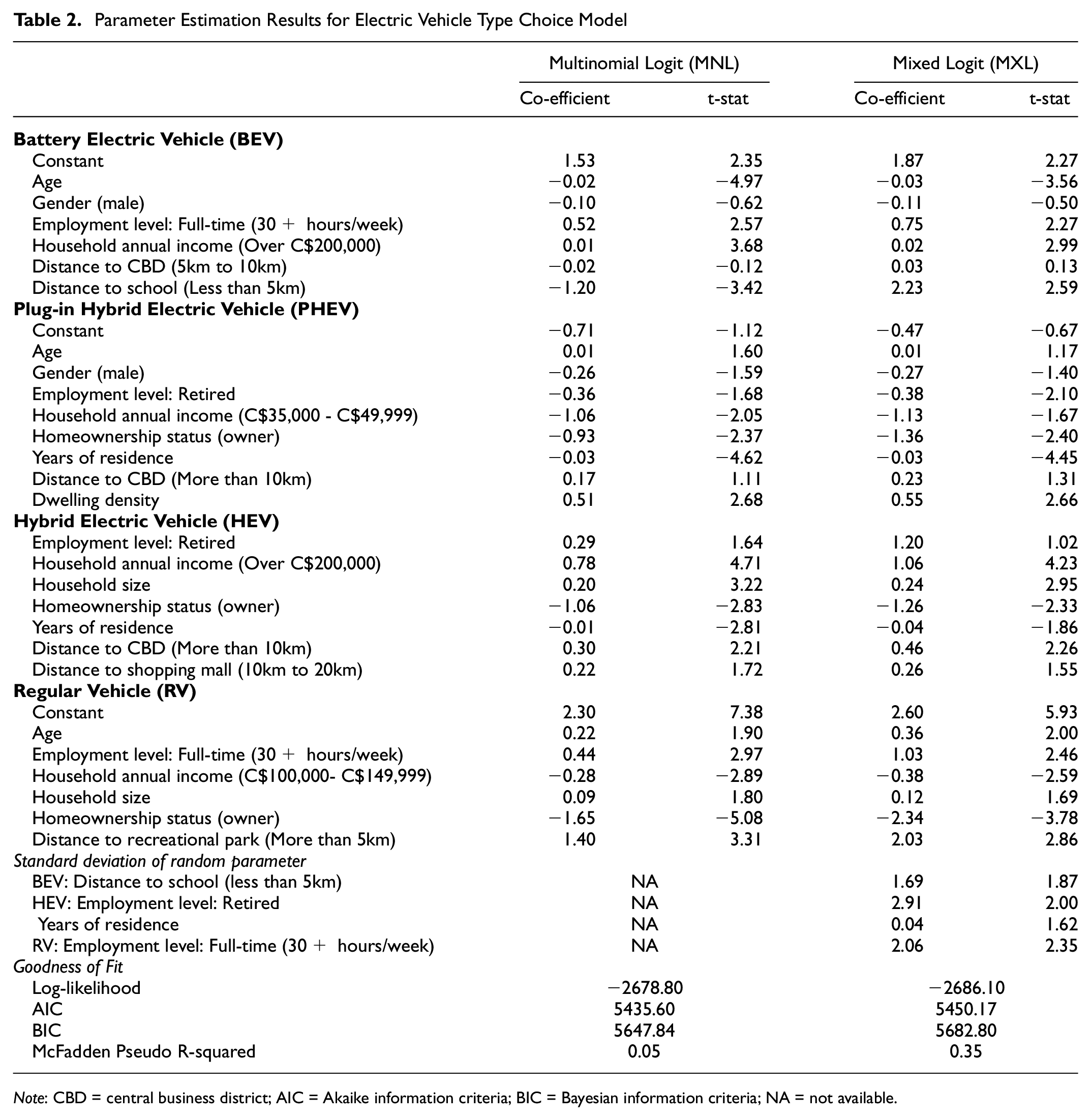
Note: CBD = central business district; AIC = Akaike information criteria; BIC = Bayesian information criteria; NA = not available.
The results show that age has a negative correlation with the adoption of BEVs, which indicates the younger generation has a higher propensity to adopt fully EVs. The younger generation is also more concerned about or aware of environmental issues. This consciousness can influence their future vehicle type choices. Households with an income level greater than C$200,000 demonstrate a higher probability of adopting BEVs. This parameter is found to be statistically significant at a 99% confidence interval. Similarly, the home to school distance (less than 5 km) illustrates a positive correlation between the BEV choice and this variable, which explains the heterogeneity among the respondents with a substantial value of standard deviation (1.87). The PHEVs consist of an internal combustion engine with an electric motor and a rechargeable battery pack that can be charged by an external power source. Males have less inclination to adopt PHEVs than females. Retired people are less enthusiastic about adopting PHEVs as well. The households in the higher-income group and full-time employees have a higher probability of choosing PHEVs because their purchase price is high. This phenomenon explains why households with lower annual income (C$35,000–C$49,000) are less likely to choose PHEVs. Dwelling density plays a significant role in the adoption of PHEVs, creating a positive coefficient value. People who live in more dense areas, such as the downtown core, are very motivated to choose PHEVs in the next five years.
HEVs include both conventional vehicles and EVs. HEVs do not require any external charging sources and have a small battery pack that recharges while running on regular fuel. Households with a higher income range (over C$200,000) and household size are found to be notable and illustrate a positive correlation with choosing HEVs. The distance to the CBD (more than 10 km) and shopping mall (10–20 km) have a positive relationship as well. The results indicate that people are choosing HEVs for longer trips as they do not require an external power source to recharge. Both retired individuals and the years of residence exhibit heterogeneity among responses; they have a higher standard deviation than the mean value. Regular vehicles consider both gasoline and diesel-driven vehicles. Age has a positive correlation with the regular vehicle type choice. The propensity to choose a regular vehicle increases with age. Older people do not feel comfortable using new technology like EVs, which is why they prefer regular vehicles over different types of EVs. Full-time workers have a positive attitude toward regular vehicles. That being said, heterogeneity is captured among the survey respondents with a standard deviation of 2.35. People who live close to recreational parks have a lower propensity to choose EVs. Homeownership status has a negative correlation to PHEV, HEV, and regular vehicle adoption. It is possible for individuals to choose a fully EV because they have the capacity to have charging infrastructure at their home locations. Overall, the younger generation, females, and households with a higher income range portray a higher probability to adopt EVs in the near future and their decision to do so can be accelerated through proper policy interventions.
Traffic Macrosimulation Model Result
To assess the traffic network impact for different scenarios, two peak periods: (1) the morning peak period (7:00–9:00 a.m.) and (2) the evening peak period (4:00–6:00 p.m.); were modeled in this study within the VISUM platform. The key performance indicators for the SDA method include the number of trips by each vehicle type, vehicle kilometers traveled (VKT), vehicle hours traveled (VHT), and average vehicle speed on different road classes. Figures 6 and 7 show a comparison of trips by different modes for the three scenarios.
Figure 8 explores the distribution of trip frequency and VKT for the three scenarios during the morning peak period. The results show that the total number of trips is projected to increase by 6.8% in 2027 and 7.4% in 2032, compared to the base year of 2022. The total distance traveled by vehicles will also experience an increase of 7.7% in 2027 and 8.4% in 2032. Despite the general growth in trips and VKT over the years, there is a trend of the share of regular vehicles in the fleet decreasing because of the adoption of EVs. By 2027, the share of regular vehicles will be 83.7%, with the remaining portion comprising EV types such as PHEVs (14%), HEVs (1.7%), and BEVs (0.6%). The total number of trips completed by regular vehicles will be 11% less in 2027 than the base year of 2022. Although the total VKT increased in 2027, only 87% came from regular vehicles, while the rest were from EVs (PHEVs—9.4%, HEVs—2.5%, and BEVs—0.9%). Furthermore, the total VKT by regular vehicles will experience a 7% reduction compared to 2022. Similarly, the total number of trips completed by regular vehicles will reduce by 26% in 2032 compared to 2022 and by 18% compared to 2027. The share of regular vehicles will be 69% in 2032, with the remaining portion comprising different types of EVs. Moreover, trips completed by EVs in 2023 will have increased further from 2027, with PHEVs accounting for 25% (14% in 2027), HEVs for 5.4% (1.7% in 2027), and BEVs for 0.9% (0.6% in 2027). Even though the total VKT increased by 8.4% in 2032 compared to 2022, the VKT from regular vehicles experienced a reduction of 23% compared to the base year. In addition, the evening peak hour trips and VKT exhibit a similar pattern to that observed in the morning peak period (Figure 9).
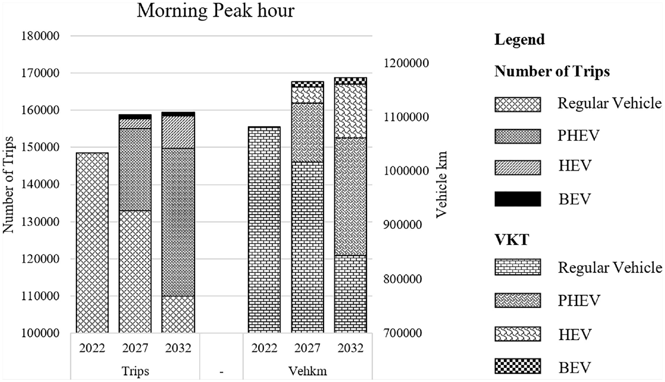
Distribution of trip frequency and vehicle kilometers traveled for different scenarios during the morning peak period.
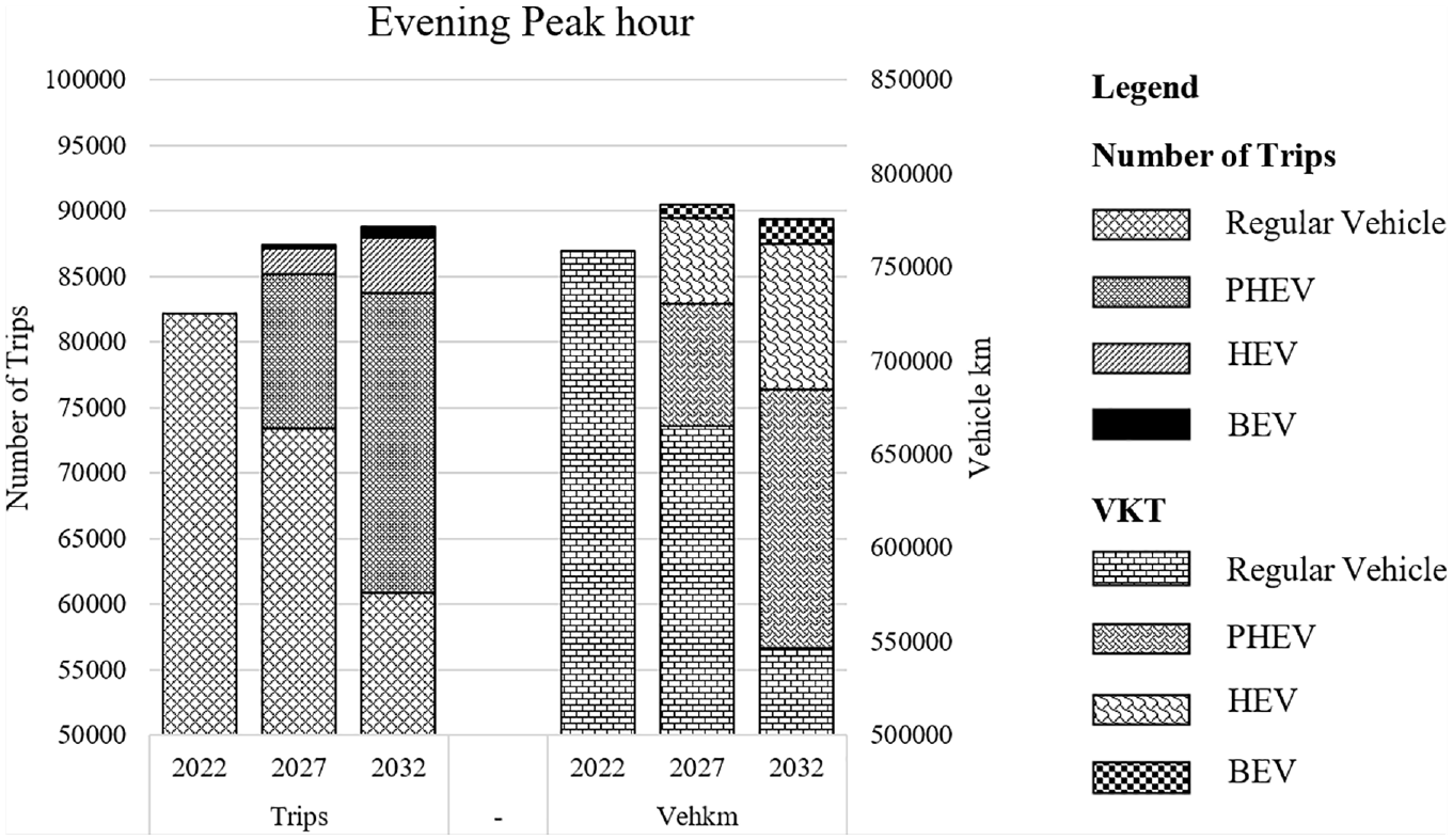
Distribution of trip frequency and vehicle kilometers traveled for different scenarios during the evening peak period.
Figure 10 illustrates the comparison of vehicle flows of regular vehicles, PHEVs, HEVs, and BEVs across the three highest volume locations under three distinct scenarios during the morning peak period. Figure 10a depicts the volume changes on Macdonald Bridge: 18.8% of trips will be by EVs in 2027 and this will increase to 34% in 2032. On Barrington Street (Figure 10b), 18.3% of vehicles will be EVs in 2027, and the share will increase to 38.3% in 2032. There is a similar pattern of change is observed in the Bedford Highway area as well (Figure 10c).
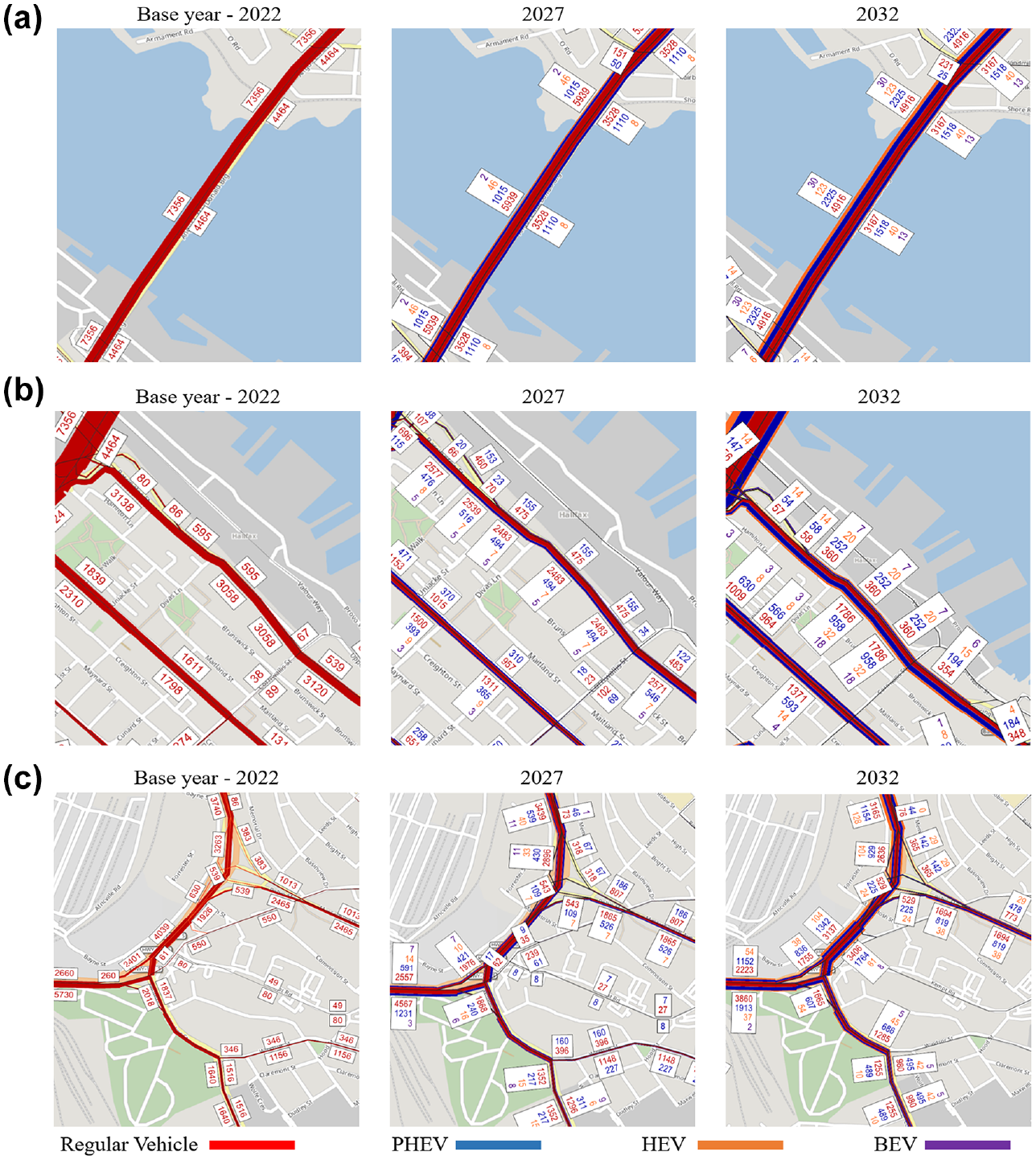
Comparison of auto trip flows for each scenario: (a) Macdonald Bridge, (b) Barrington Street, and (c) Bedford Highway/Windsor Street/Massachusetts Avenue.
Emission Result
Zonal Level Emission Reduction
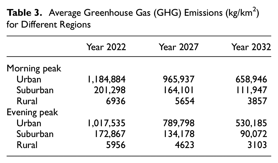
GHG emissions on the zonal level are calculated using the MOVES platform. They are mostly concentrated in the urban area, as shown in Table 3. It provides the change of GHG emissions for two other different scenarios for the years 2027 and 2032. GHG emissions are reduced by a significant amount by the incremental adoption of EVs in the network. Figures 11 and 12 demonstrate the distribution of GHG emissions for all TAZs considering morning and evening peaks. The densely populated area in the HRM and mixed land use pattern are the underlying reasons behind the highest concentrations of GHG emissions in the urban core. In 2027, an overall emission reduction of 18.5% and GHG emissions of 22.4% are noticed during the morning and evening peak periods compared to the base year of 2022. In addition, 31.8% and 32.9% of GHG emissions will be reduced in 2032 with respect to 2027 during the morning and evening peak periods.
Average Greenhouse Gas (GHG) Emissions (kg/km2) for Different Regions
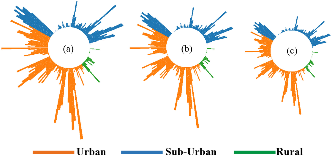
Zonal level greenhouse gas as CO2 equivalent emission reductions for years (a) 2022, (b) 2027, and (c) 2032 for the morning peak period.
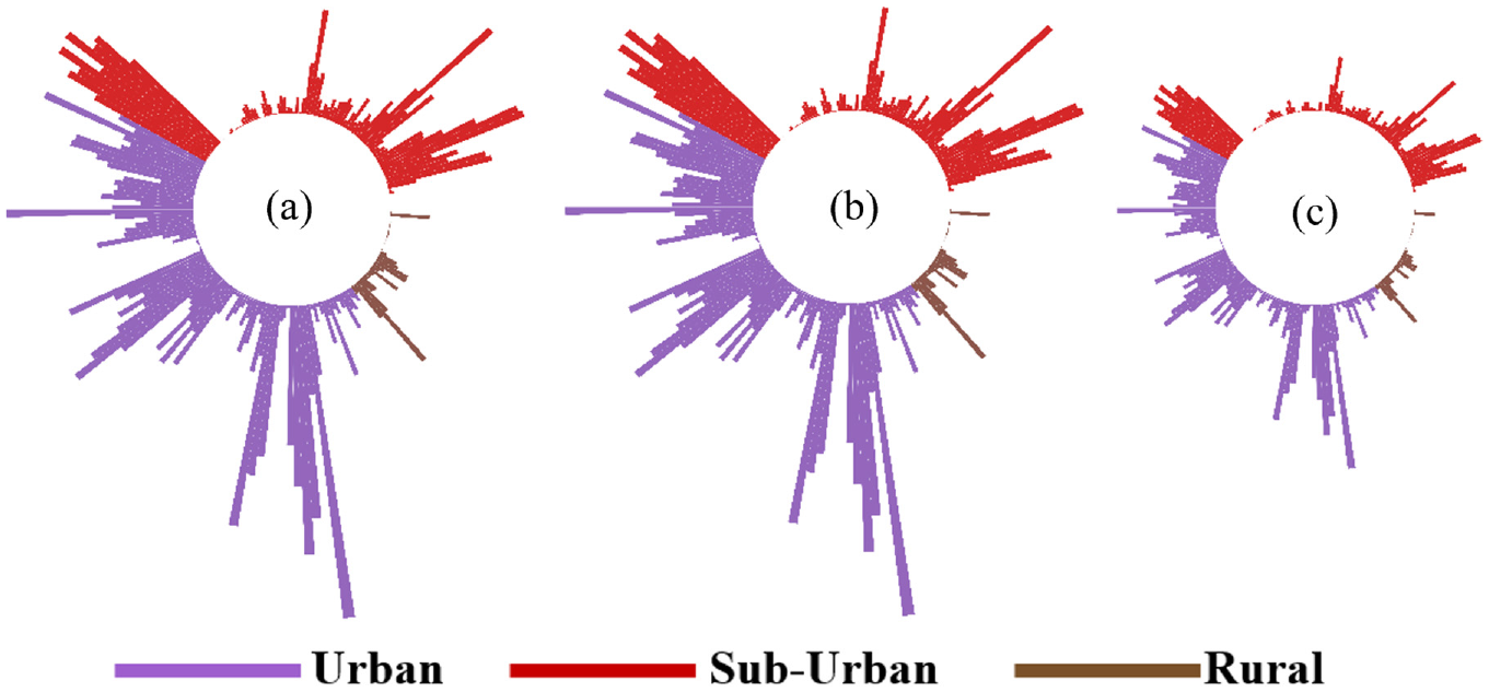
Zonal level greenhouse gas as CO2 equivalent emission reductions for years (a) 2022, (b) 2027, and (c) 2032 for the evening peak period.
Spatial Distribution of GHG Emissions
The spatial analysis of the emission data is conducted using ArcGIS Pro to represent the GHG emission density for each TAZ. Zonal emission values vary from 0 to 4,000,000 kg/km2. To address a uniform comparison among the density distribution of GHG emissions across different zones, this research considers a low level of GHG emissions to be less than 150,000 kg/km2. Similarly, if the emission level is between 1,000,000 and 1,150,000 kg/km2, it represents the medium level, and GHG emissions of more than 2,000,000 kg/km2 are considered as a higher level of emissions. Figures 13 and 14 show the comparison of GHG emissions as CO2 equivalent density between two peak periods among the three scenarios (2022, 2027, and 2032). Both figures show that the highest concentration of GHG emissions will occur in the downtown core of Halifax and Dartmouth in the base year of 2022. However, all TAZs will experience a considerable decrease in emissions because of the adoption of EVs over time. The changes in emission density in 2027 and 2032 clearly indicate the positive impact of EVs on GHG emissions.
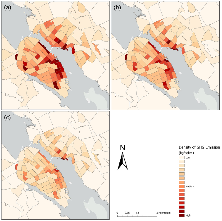
Comparison of greenhouse gas (GHG) as CO2 equivalent emission density among (a) 2022, (b) 2027, and (c) 2032 for the morning peak period.
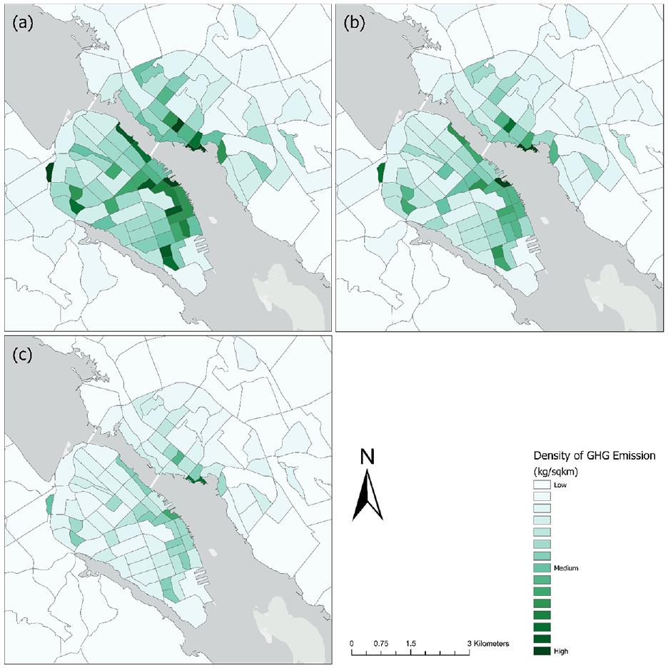
Comparison of greenhouse gas (GHG) as CO2 equivalent emission density among (a) 2022, (b) 2027, and (c) 2032 for the evening peak period.
Conclusions
This study develops a comprehensive modeling framework to examine the impact of vehicle electrification on traffic networks and vehicular emissions. The tool coupling technique was adopted to integrate an activity-based travel demand forecasting model (iTLE) updating the vehicle type choice model with the traffic network simulator developed in PTV VISUM and EPA’s MOVES3.0. Coupling of these models fulfills the need for an operational integrated model for the HRM for scenario assessments. The study utilizes the 2022 HaliTRAC survey data to formulate a random utility-based econometric model, using a MXL model for an EV type choice model. This research also simulates three different scenarios incorporating EV adoption to shed some light on the impact on the network and vehicular reduction.
Results suggest that younger generations and households with a higher annual income are highly interested in adopting EVs, which stems from their concern for the environment. In contrast, older people are comfortable using regular gasoline or diesel-driven vehicles. Although households with lower incomes have a lower propensity to adopt EVs, residents living in dense areas are highly motivated to purchase PHEVs in the near future. Moreover, people prefer to use HEVs for long-distance travel, arguably because they do not require any external power source to recharge. This study forecasts a rise in total vehicle trips (6.8% by 2027, 7.4% by 2032) and vehicle distance traveled (7.7% by 2027, 8.4% by 2032) during the morning peak period. However, the share of regular vehicles declines because of EV adoption, reaching 83.7% by 2027 and 69% in 2032. The share of EVs in the vehicle fleet will increase over the years. In 2027, EVs will comprise 16.3% (PHEVs 14%, HEVs 1.7%, and BEVs 0.6%), and by 2032, it will rise to 31% (PHEVs 25%, HEVs 5.4%, and BEVs 0.9%). Evening peak trends follow the morning peak pattern. Because of the EV adoption over time, overall GHG emissions will be reduced by 18.5% of in 2027 compared to the base year of 2022 and will reduced by 31.8% in 2032 compared to the year 2027 during the morning peak period. A similar trend is noticed for the evening peak period, which will have 22.4% and 32.9% reductions in GHG emissions in 2027 and 2032, respectively. The highest concentration of GHG emissions is noticed in the densely populated mixed land use urban core comprising the downtown core of Halifax and Dartmouth. However, all TAZs will experience a considerable decrease in emissions, indicating the positive impact of EVs on GHG emissions. The results have some critical policy implications as well. Households with an income level exceeding C$200,000 show a higher likelihood of adopting BEVs, indicating financial incentives such as tax credits or rebates could serve as powerful motivators for greater adoption of EVs. In Nova Scotia, the Ecology Action Centre (EAC) strategy proposes various financial incentives that the provincial and federal governments should implement to increase EV adoption ( 37 ). As age negatively correlates with EV adoption, the younger generation shows a greater inclination toward adopting EVs. To boost EV adoption among this demographic, implementing awareness campaigns that highlight the role of EVs in addressing climate change, offering age-specific incentives, and providing additional incentives for those choosing an EV as their first vehicle could be effective strategies. Considering the positive correlation between EV adoption and dwellers in dense areas, it is advisable to introduce priority parking for EVs in urban areas.
Furthermore, the development of a robust and widespread charging infrastructure could attract people to EVs. The study contributes some novel insights related to the development of an integrated tool, even though it has certain limitations. The EV type choice model is developed following individuals’ socio-demographic characteristics, neighborhood characteristics, and accessibility measurements; this model is not calibrated/validated so far. Subsequent investigations will encompass the implementation of multi-tiered calibration/validation methodologies, coupled with sensitivity analyses or the assessment of the elasticity effects of model parameters, with the aim of enhancing the efficacy of the integrated activity-based model, the iTLE model. The study also does not consider any vehicle attributes related to different categories of EVs, such as the driving range, charging cost, and annual maintenance cost, among others. This phase of the investigation exclusively focuses on tailpipe emissions, neglecting to incorporate the implications of non-exhaust emissions originating from plausible diverse sources, including tire and brake abrasion, road surface deterioration, and aerosolization of fluids, among other factors. Future studies should incorporate this aspect along with the power source of EV charging stations to simulate more informed decisions made by the respondents. The study currently employs dynamic stochastic assignment, which does not consider junction impedance effects in the assignment process. In the future, adopting SBA in VISUM could address this limitation. The emission model only considered passenger cars for calculating emissions. Future work should incorporate a multimodal transport network, including the estimation of a 24-hr GHG emission profile instead of two peak periods. In addition, the calibration and validation of the traffic macrosimulation model and the emissions model will need to be done to develop a holistic approach, ensuring the credibility of the model. Nevertheless, the modeling system developed in this study successfully integrates multiple processes of travel demand, EV adoption, traffic flow, and emission estimation, yielding an operational model for the HRM. Moreover, the results from this analysis support policy interventions such as purchase subsidies, increased charging infrastructure, and tax rebates to help encourage the adoption of EVs among Halifax residents.
Footnotes
Author Contributions
The authors confirm contribution to the paper as follows: study conception and design: H. Shahrier, M.A. Habib; data collection: M.A. Habib, H. Shahrier; analysis and interpretation of results: H. Shahrier, V. Arunakirinathan, F. Hossain, M.A. Habib; draft manuscript preparation: H. Shahrier, V. Arunakirinathan, F. Hossain, M.A. Habib. All authors reviewed the results and approved the final version of the manuscript.
Declaration of Conflicting Interests
The author(s) declared no potential conflicts of interest with respect to the research, authorship, and/or publication of this article.
Funding
The author(s) disclosed receipt of the following financial support for the research, authorship, and/or publication of this article: This work was supported by the Climate Action Awareness Fund (CAAF), Natural Sciences and Engineering Research Council (NSERC)—Discovery Grant and the Halifax Regional Municipality (HRM).