
Abstract
Particulate matter with a diameter of 2.5 microns or less (PM2.5) has significant impacts on human health, making it essential to understand its spatial and temporal variations. This study focuses on developing land use regression (LUR) models and improving their performance in predicting PM2.5 concentrations in an urban setting. In this study, air quality data were collected using a sensor on a courier truck in downtown Toronto. Extreme gradient boosting (XGBoost), a machine learning algorithm, was employed to address limitations in traditional linear regression based LUR models, incorporating predictors such as land use, meteorology, and emissions to build robust models. A total of 27 models were trained, with varying road segment lengths, predictors, and outlier treatment thresholds. Three models tested the impact of road segment length on model predictions. Eight models examined the effect of removing outliers with different thresholds, revealing that appropriate thresholds improve accuracy. Ten models assessed the addition of emission and traffic data, which did not enhance performance, likely because of overlapping effects with other predictors. In six models, time-variant predictors such as time of day, month, humidity, wind speed, temperature, and pollutant concentrations from stationary stations were included. Adding these predictors significantly improved model performance, highlighting the complex relationships in LUR models for PM2.5 predictions and offering valuable insights for air quality assessment.
Keywords
Air quality stands as a critical environmental concern, affecting millions of individuals worldwide. Among the air pollutants, particulate matter with a diameter of 2.5 microns or less (PM2.5) severely affects human health ( 1 ). Understanding spatial or spatiotemporal pollutant concentrations plays a vital role in implementing effective mitigation strategies and in developing accurate exposure surfaces to support the analysis of long-term health effects ( 2 ). Reference air quality stations provide reliable air pollutant concentration information, but they have limitations as data is available at limited points ( 1 ). To overcome these limitations, researchers use models such as geostatistical interpolation, photo-chemical dispersion, and land use regression (LUR) to assess air pollution exposure and its associated health effects in urban areas ( 3 ). While geostatistical interpolation and dispersion models are valuable, their resolution is often coarse, making them less suitable for capturing small-scale urban variability that is crucial in exposure assessment ( 4 ). In contrast, LUR models have become popular for quantifying intraurban variation in air pollutant concentrations, offering simplicity and the ability to predict fine-scale pollution variations that can reduce exposure measurement errors ( 4 , 5 ). The main components of LUR models include monitoring data, geographic predictors, model development, and validation ( 5 , 6 ). Traditionally, LUR models have relied on stationary air quality monitors, but these methods fail to capture small-scale spatial variations in pollutant concentrations. Mobile monitoring offers an alternative with better spatial coverage, though it presents challenges in addressing temporal variability ( 6 , 7 ).
Criticism of linear regression based LUR models includes limited flexibility and difficulty in incorporating highly correlated predictors ( 8 ). Studies have explored machine learning models, such as neural networks, support vector machine, and tree-based models, which improve accuracy and handle multicollinearity ( 8 , 9 ). Predictors for LUR models include land use, meteorology, pollutant emissions, and built environment characteristics. Common predictor variables are traffic, population density, land use, topography, and location ( 10 ). Understanding the impact of such predictors is crucial for improving models and capturing spatiotemporal variation. Studies have used various methods to assess LUR model performance. Common approaches include cross-validation techniques such as leave-one-out cross-validation (LOOCV), where each data point is tested once while the model is trained on the rest. Regional cross-validation (RCV) evaluates model error by leaving out data points within a specific region and predicting concentrations there ( 11 ). Some studies use external data for validation, noting that a high training R2 may not correspond to a high test-set R2 when estimating long-term average exposure ( 12 ).
Across the literature, different sets of LUR models, predictors, and postprocessing of data have been used to improve predicted long-term or short-term exposure surfaces. In a study by Messier et al. ( 6 ), nitric oxide (NO) and black carbon (BC) measured by mobile monitoring and a land use regression-kriging (LUR-K) was implemented on part of a dataset to predict concentration of pollutants at unobserved locations. Kerckhoffs et al. ( 13 ) compared the performance of a simple linear regression, several algorithms based on regularization, and several machine learning algorithms (random forest, boosting, and bagging) to predict long-term ultrafine particles (UFP). They showed that machine learning models had better performance for their data. In another study, Kerckhoffs et al. ( 14 ) implemented three models (supervised stepwise regression, Least Absolute Shrinkage and Selection Operator(LASSO), and random forest) to predict long-term average UFP by using a deconvoluting method to separate local UFP contributions from background concentrations. In another study by Liu et al. ( 8 ), a linear regression was compared with gradient boosting decision tree (GBDT) models. The study showed that the GBDT model captured non-linear relationships and explained more of the variations in the pollutant concentrations ( 14 ). In recent years, more complex machine learning algorithms such as artificial neural networks (ANN) have been used for prediction. In a study by Wang et al. ( 15 ), the performance of two machine learning approaches, ANN and gradient boost, were compared with simple linear regression LUR using five data segmentation schemes. Machine learning methods exhibited superior performance over a simple LUR model. In the studies conducted by Ren et al. ( 16 ) and Wong et al. ( 17 ), various machine learning methods and simple LUR models were assessed. Both studies arrived at the conclusion that the extreme gradient boosting (XGBoost) algorithm outperformed the other approaches.
LUR models are widely used in air quality research to estimate pollutant concentrations in areas lacking direct monitoring data. By incorporating spatial predictors such as land use types, traffic density, population distribution, and meteorological data, LUR models can effectively predict pollution levels beyond measurement locations (whether fixed or mobile), including off-road environments. For instance, Padhi and Kumar ( 18 ) discusses the application of LUR models in air pollution assessment, highlighting their effectiveness in capturing spatial variability. Similarly, research by Hankey and Marshall ( 19 ) demonstrates the successful modeling of on-road particulate air pollution, including particle number, black carbon, and PM2.5, using LUR techniques based on mobile monitoring data. Their findings highlight the effectiveness of LUR models in capturing spatial variability of pollutants across urban settings. While uncertainties may arise when extrapolating to areas far from monitoring points, LUR models have been validated in diverse settings, demonstrating their robustness in capturing spatial trends across urban and suburban environments. These strengths make LUR models valuable for understanding exposure in off-road locations.
In this study, we used the XGBoost algorithm to develop multiple models with the aim of predicting concentrations of PM2.5. To gather the data for developing the models, a sensor was installed on a courier truck operating in Toronto, Canada. The primary focus of this research is to investigate the possibility of enhancing prediction ability of the model by employing diverse predictors and addressing outliers. By constructing distinct models for varied sets of input data as predictors, we conducted comparisons to understand the impact of these predictors and modifications on the overall performance of the model. Additionally, the feasibility of utilizing delivery vehicle routes for constructing a LUR model to predict exposure surfaces was assessed. The study outcomes can be leveraged to investigate the potential of a fleet serving as a mobile monitoring platform.
Beyond contributing to the methodological development of exposure surfaces, this study offers valuable insights for urban planning, public health, and community-level air quality management. Previous research has demonstrated the value of LUR models in identifying urban air pollution hotspots and supporting interventions to mitigate health risks associated with air pollution. For instance, Hoek et al. ( 11 ) reviewed the application of LUR models in air pollution epidemiology, highlighting their effectiveness in exposure assessment and their potential to inform public health policies. Similarly, Jerrett et al. ( 20 ) used LUR models to examine the relationship between air pollution and mortality in urban areas, underscoring their role in exposure analysis and public health risk assessment. Furthermore, Lu et al. ( 21 ) discussed the application of LUR models for identifying air pollution hotspots in urban environments, emphasizing their value in supporting population health by guiding urban planning decisions. By using low-cost mobile sensors and implementing advanced LUR modeling techniques, our findings allow for a more nuanced understanding of PM2.5 variability across urban areas, which can help inform effective strategies to reduce population exposure and promote healthier urban spaces.
Methods
Study Area
This study is set in the city of Toronto, located on the north shore of Lake Ontario in southeastern Canada and with a population of over 2.7 million, making it the largest city in the country. Toronto experiences a temperate climate with distinct seasons. This city has a relatively flat topography, especially in the downtown core and along the lakeshore. Air quality in Toronto can vary depending on several factors, including weather, traffic, industrial activity, seasonal influences, and proximity to major sources like Toronto’s municipal expressways and provincial highways or its two airports: Toronto Pearson International Airport located west of the city and Billy Bishop Toronto City Airport on the Toronto Islands. Among all the sources, traffic emissions are a major local source of air pollution in Toronto. This includes emissions from cars, trucks, buses, and other forms of transportation.
Data Collection and Preprocessing
We conducted a mobile monitoring campaign in Toronto by installing a sensor on a truck operated by Purolator, a courier and package delivery company in Toronto, to capture spatiotemporal variation of ambient PM2.5. The mobile monitoring campaign took place between June 21, 2022, to January 11, 2023.
The sensor, manufactured by Geotab, a telematics and fleet management company, uses a Honeywell HPMA 11S50 low-cost sensor. The HPMA 11S50 sensor is capable of measuring ambient particulate matter (PM) concentrations. It can detect and quantify real-time PM2.5 and PM10. In fact, the sensor is designed to capture a broad spectrum of particulate concentrations, suitable for urban air quality monitoring. It responds rapidly to changes in PM levels, ensuring near real-time data collection. The sensor operates reliably across a wide range of temperatures and humidity conditions. It was factory-calibrated to ensure accurate and consistent measurements ( 22 , 23 ). This sensor is integrated into a Geotab unit which also includes a SGX Sensortech MiCS-4514 to collect NO2 concentrations and Bosch Sensortech BME280 to collect temperature, humidity, and atmospheric pressure ( 9 ). Moreover, Geotab reports a wide range of vehicle telematics data such as GPS location, fuel level, and other on-board diagnostics (OBD). The sensor reports a record whenever a property changes, for example whenever PM2.5 concentration changes, a new record is reported. The instruments were calibrated by the manufacturer before installation. To minimize the risk of self-pollution from the truck’s exhaust emissions, the PM2.5 sensor was strategically placed with the airflow intake positioned on the top of the truck’s right window, facing outward. This positioning was chosen to avoid direct exposure to exhaust gases and ensure that the sensor primarily measured ambient air quality rather than pollutants emitted by the vehicle itself.
To assess the reliability of the sensor readings over time, we compared PM2.5 concentrations recorded by the mobile sensor with data from a near-reference monitoring station located along College Street, a busy arterial road on the campus of the University of Toronto, during periods when the truck operated near this station (within a 200-m radius). This station uses a Thermo Scientific 5030 SHARP Synchronized Hybrid Ambient Real-time Particulate Monitor; its location is presented in Figure 1. This comparison helped verify the consistency and accuracy of the mobile measurements, providing validation for the sensor's stability and accuracy throughout the study period.
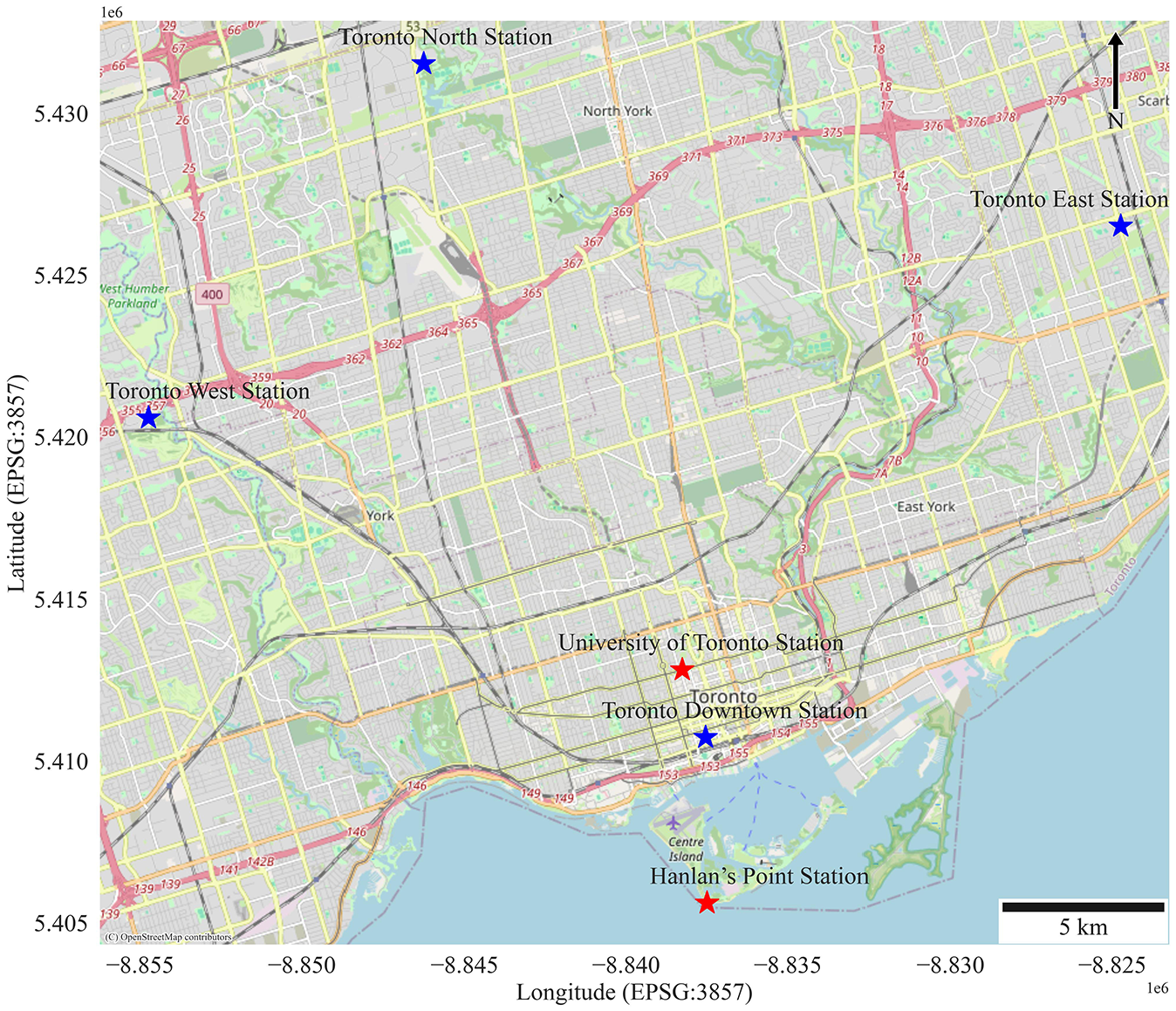
Map featuring the locations of monitoring stations in Toronto. The near-reference monitoring stations (Hanlan’s Point (HN) Station and University of Toronto (UofT) Station) are pinpointed along with the four regulatory monitoring stations operated by the Ontario Ministry of Conservation and Parks (Toronto Downtown Station, Toronto East Station, Toronto North Station, and Toronto West Station).
The concentration of PM2.5 was recorded for a total of 56,577 data points while the truck was in operation. The truck was operating mostly between 7 a.m. and 7 p.m. and 20% of the data points were recorded during the morning (7 to 11 a.m.), 41% around midday (11 a.m. to 3 p.m.), 31% in the afternoon (3 to 7 p.m.), and the remaining were recorded outside those hours. The truck mostly operated in the downtown area. During the campaign, the truck was operational for approximately 300 h over the 6-month period, as a result of variable daily operational hours of the Purolator delivery vehicle, which did not consistently follow an 8-h schedule. However, the PM2.5 sensor was active for only 157 h. This discrepancy arises from instances where drivers inadvertently forget to turn on the sensor. These factors led to reduced data collection time over the 6-month period. Another observation from our data analysis is the presence of records for 5,767 distinct minutes (equivalent to 96 h). This indicates that the sensor didn't continuously report data throughout its 157-h active time. The gaps in the data correspond to moments when the sensor did not report new values given the absence of significant concentration changes.
Each data point consists of a pair of x.y coordinates associated with a PM2.5 concentration. For this reason, we averaged all observations corresponding with each road segment, defining those segments using different methods. In the first method, the observations were aggregated for each road segment (defined from one intersection to another) from a road network shapefile for Toronto. Then the center of each road was identified, and buffers were created around each point to compute model predictors. As a result, all data points were assigned to approximately 1050 road segments. In the second and third methods, segments were defined at every 50-m and 100-m interval, with the average concentration computed for all readings associated with these segments. With a 50-m aggregation, the total number of segments is 1,673, and with a 100-m aggregation, it is 705. These three methods were used to evaluate the impact of spatial aggregation. We used the 50-m segment as the base case against which all models will be compared since it refers to the highest resolution. These three methods of aggregation have been employed by other studies ( 4 , 6 , 24 ).
Generation of Predictor Variables
Several LUR models were developed using different sets of predictors to evaluate the impact of choosing predictors on the performance of LUR models. We divided our predictors into three categories including specific to a location predictor, traffic related predictors, as well as weather and air quality related predictors which can change temporally. To calculate predictors, varying buffer sizes (50, 100, 200, 250, 300, 500, 1000, 2000 m) were created around each segment mid-point (based on the three methods for data aggregation). The calculation of predictors involved the calculation of area, length, or number of land use types and traffic related variables within each of these buffers, computation of distances to important places in the city from the buffers’ centers, and temporally changing variables (weather and regional air quality).
Predictors that accurately explain emissions or traffic can affect LUR models and their effectiveness in estimating pollution concentrations ( 8 ). In this study, LUR models were created to assess the contrasting effects of utilizing two data sources for traffic and emissions. In one model, traffic volume and emissions for nitrogen oxides (NOx) from the GTAModel, an activity-based model for the Greater Toronto Area which uses the Equilibrium Multi-Modal Environment (EMME) traffic assignment package, were included as predictors ( 25 , 26 ). Then, four models were developed by including annual average daily traffic (AADT) data instead of emission data. The AADT data used in this study was developed by Ganji et al. ( 27 ) by using traffic count data to calculate AADT instead of a travel demand model. The AADT data was improved by Ganji et al. ( 28 ) using aerial imagery. Four models were trained with AADT data from four different years (2017, 2018, 2019, 2020).
To address temporal variability of PM2.5 concentrations, several models were trained by adding new predictors. For this purpose, we utilized data from two near-reference monitoring stations, one situated at the University of Toronto and the other one near Lake Ontario, at Hanlan’s point, south of the city. These monitoring stations provided environmental variables including humidity, wind speed, temperature, regional PM2.5, and gaseous pollutants such as NOx (nitrogen oxides), NO (nitric oxide), and NO2 (nitrogen dioxide). We also added time of day as three categories (morning, midday, and afternoon), and day of week and month for examining the possibility of capturing daily, weekly and seasonal trends in PM2.5. All the predictors, their categories, and type of measurement are detailed in Table 1.
Summary of Predictors Categorized into Land Use-Related Variables (e.g., Area, Population, Proximity), Traffic-Related Variables (e.g., Road Lengths, Traffic Counts, Emissions), and Temporally Changing Variables (e.g., Time of Day, Month, Weather Conditions)
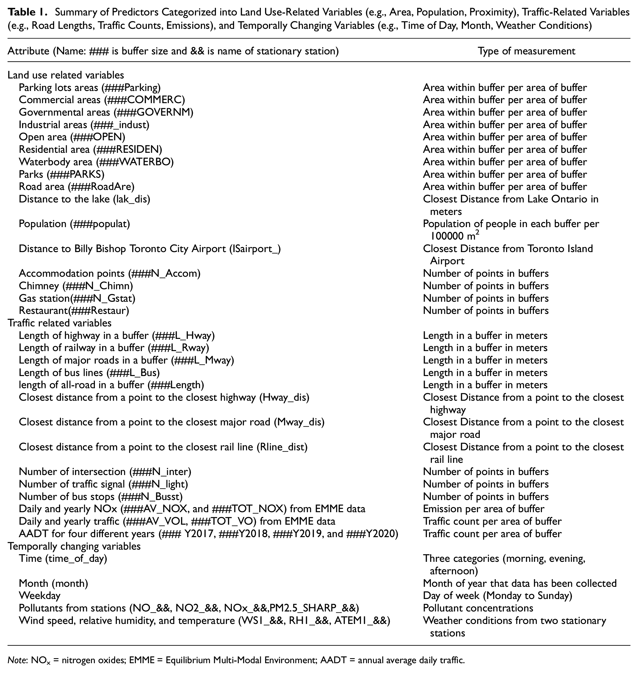
Note: NOx = nitrogen oxides; EMME = Equilibrium Multi-Modal Environment; AADT = annual average daily traffic.
Land-Use Regression Modelling
In this study, the XGBoost model, which is a tree-based machine learning method, was trained using different sets of predictors to predict long-term PM2.5 exposure surfaces and to study the impact of using different sets of predictors on the model performance. The XGBoost model can capture non-linear relations between predictors ( 15 , 16 ). The importance of predictors can be extracted from this model using different feature importance measures. In this study, the Python libraries’ scikit-learn and XGBoost were used ( 29 ). The grid search method was used to tune our models. After tuning and choosing the best model, we used a feature importance method to assess the impact of different features on model output and predictive performance.
To assess model accuracy, the dataset was partitioned into training and testing sets, with 20% allocated for testing. The model was trained and evaluated at the same time using a 10-fold cross-validation (CV) approach in combination with grid search for hyperparameter tuning. In fact, by using this method, the training data set was divided into 10 subsets, and the model was trained and evaluated 10 times. Each time, one of the 10-folds is used for testing the model and other folds for training. The model performance was averaged for all these 10 models to provide an overall assessment of its accuracy and generalization. After finding the best models and their hyperparameters, the models were tested by using the 20% test set which the model had not seen during training and tuning. The best coefficient of determination (R2) values for the test set and 10-fold CV were compared for the different models.
Finally, we conducted a validation analysis by comparing the models’ predicted PM2.5 concentrations with the average of measurements during the sampling period from four regulatory monitoring stations in Toronto, operated by the Ontario Ministry of Conservation and Parks (excluding the near-reference station used for sensor comparison); the locations of these stations are identified in Figure 1. We computed the accuracy of model predictions, calculated as
The impact of deleting outliers on XGBoost performance was evaluated. To evaluate the effect of deleting outliers on the performance of LUR models, we compared our models when we delete outliers larger and less than specific percentiles. We deleted PM2.5 concentrations when they were larger than 99.7th, 99th, and 95th percentiles and less than 5th (all zero records), 10th, and 20th. We trained eight models by using various combinations of these thresholds, removing data exceeding or falling below the specified values as necessary and for some models, we exclusively utilized either the upper or lower threshold for data removal. Three models involved the removal of data greater than the 99th, 99.7th, and 95th percentiles (referred as Outlier_1, 2, 3). Another set of three models focused on removal of data greater than the 95th percentile and less than the 5th percentile, greater than the 95th percentile and less than the 10th percentile, and greater than the 95th percentile and less than the 20th percentile (referred as Outlier_4, 5, 6, respectively). Additionally, one model exclusively removed data falling below the 5th percentile (all zeros) (Outlier_7), while another model removed data greater than the 99.7th and less than the 5th percentiles (Outlier_8).
To assess the influence of incorporating emission and traffic count predictors on the performance of the model, we extended our analysis. In one model, we incorporated both emission and traffic count data from the GTAModel. Additionally, we included traffic count data as AADT for four different years (2017, 2018, 2019, 2020) into four separate models. These predictor sets were integrated not only into the base case model, but also into the model configuration where we removed data points less than 5th percentile (remove all zeros) and all data points greater than the 95th percentile. We also tested the impact of adding emission and traffic count predictors to the Outlier_4 model.
To handle and capture temporal variation in the concentration of the pollutants in the models, we have assessed several models with different predictors. In one model (named model_time) time of day represented as three categorical variables (morning, midday, afternoon) was considered. In another model (named as day_month) day of week (Monday to Sunday) and month (1–12) were added as predictors. Moreover, four different models (named as Station_1 to 4) were developed by adding data from stationary stations as predictors. In the Station_1 model, hourly average relative humidity, wind speed and weather temperature from two stations (HN Station and UofT Station) were added to the base case as predictors; in the Station_2 model, hourly average relative humidity, wind speed and ambient temperature along with NO, NO2, NOx and PM2.5 concentrations from the two stations were added as predictors; in the Station_3 model, all the predictors from Station_2 model using data less than 95th percentile and higher than 5th percentile were used; and for Station_4 model, we added time of day as three categories to the setting of Station_3 model.
Including the different methods of data aggregation, use of predictors, and treatment of outliers, we end up with 27 models, summarized in Figure 2.
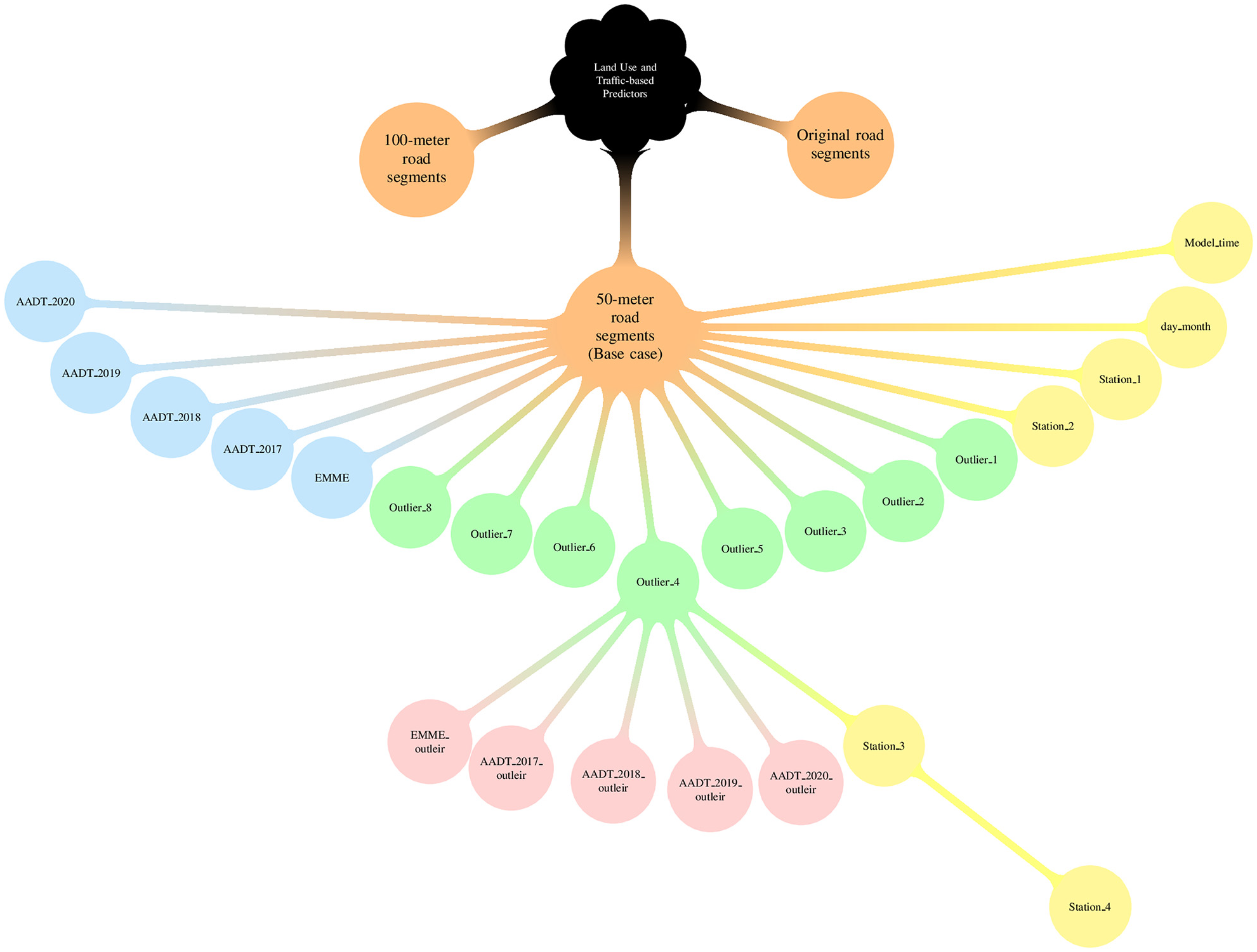
Overview of the 27 models categorized by key factors and represented in distinct colors: models evaluating (1) road segment length (orange), (2) outlier treatment (green), (3) emission and traffic data incorporation (blue), (4) combined emission/traffic data with outlier treatment (red), and (5) temporally changing predictors (yellow).
Results and Discussion
Sensor Performance
The comparison between the PM2.5 values recorded by the mobile sensor and the regulatory monitoring station yielded an R2 value of 0.63. This suggests reasonable alignment between the mobile and stationary measurements, though variability is still present. A significant factor influencing this correlation is the number of records per minute and the proximity of the truck to the station, as only records collected within a 200-m radius of the station were included in this comparison. Minutes with a higher density of second-by-second records tend to show averaged readings closer to the station's data, as more frequent measurements reduce random fluctuations (Figure 3). Conversely, minutes with fewer records or greater distances may be more affected by transient conditions, leading to less consistent alignment with the stationary measurements.
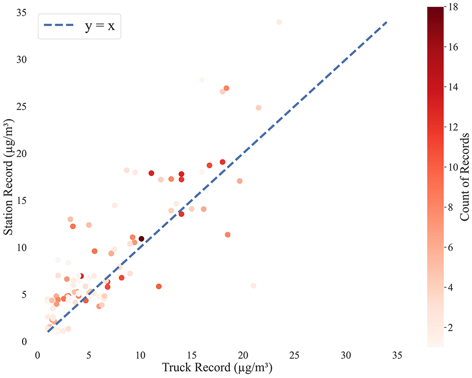
Scatter plot of PM2.5 concentrations recorded by the mobile sensor versus the University of Toronto monitoring station, with color indicating the number of measurements per minute for the sensor installed on the truck. Station records represent average PM2.5 concentration per minute. The dashed line (y = x) represents perfect agreement.
Descriptive Statistics
Our data analysis shows an average PM2.5 concentration of 9.56 µg/m3 with a standard deviation of 14.34 µg/m3, ranging from zero to a maximum of 1096 µg/m3, suggesting potential measurement errors at high levels. The high standard deviation underscores the variability in air quality within downtown Toronto, reinforcing the importance of effective analysis to capture variability. Figure 4a illustrates the box plot for PM2.5 concentrations for each sampling day. The data reveals significant variation between and within days, without a clear trend between summer and fall.
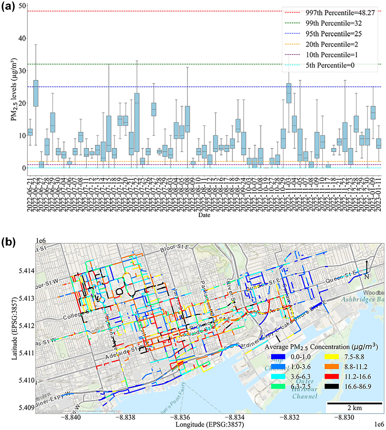
(a) Distribution of PM2.5 measurements. (b) Average PM2.5 concentration per road segment.
Figure 4b displays the distribution of average PM2.5 concentrations on road segments. This figure shows the complex spatial variability of PM2.5, which may be influenced by both spatial and temporal factors, considering that not all segments were sampled simultaneously. Based on Figure 4b, the concentration of PM2.5 in areas closer to the Toronto downtown core exhibit elevated concentrations when compared with regions farther from the city center, such as the eastern part of the city. Figure 4, a and b , provides evidence that pollution levels change within short distances and time periods, affected by weather, local emissions, and the layout of the city. These small-scale urban variabilities can be captured using LUR models ( 5 ).
Base Model
The base case uses a 50-m road segment aggregation, chosen as the benchmark for comparison. This fine resolution increases data points for training and captures spatial variability. It serves as a foundation for evaluating other aggregation methods. The R2 for the base-case model, yielded a value of 0.249 for the test dataset and 0.251 for the 10-fold CV. The SHapley Additive exPlanations (SHAP) summary plot for the base model (Figure 5) highlights key predictors influencing PM2.5 concentrations, such as road area in small buffers, proximity to major roads, and intersection density. These predictors align with the concentration sensitivity to localized factors, demonstrating its ability to capture the intricate impacts of urban infrastructure and traffic emissions on air quality.
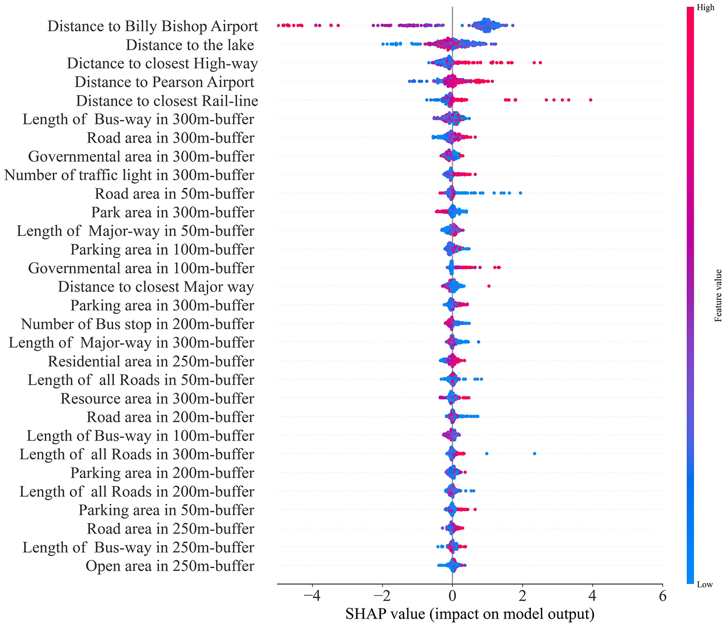
SHapley Additive exPlanations (SHAP) summary plot for top 30 features of the base model ranked by their importance. Every point represents a SHAP value, reflecting the influence of a feature on the model output for a specific observation. The color of each dot indicates the value of the corresponding independent feature, ranging from low (blue) to high (red). Higher SHAP values for features suggest elevated levels of PM2.5.
Variations on Base Model
The results of the 27 different models tested, which included three data aggregation methods, eight outlier treatment methods, five local traffic emissions data sources, five local traffic emissions data sources applied with an outlier treatment method, and six models with temporal variables, are presented in Figure 6. The R2 values for the test set and 10-fold CV for these models are reported.
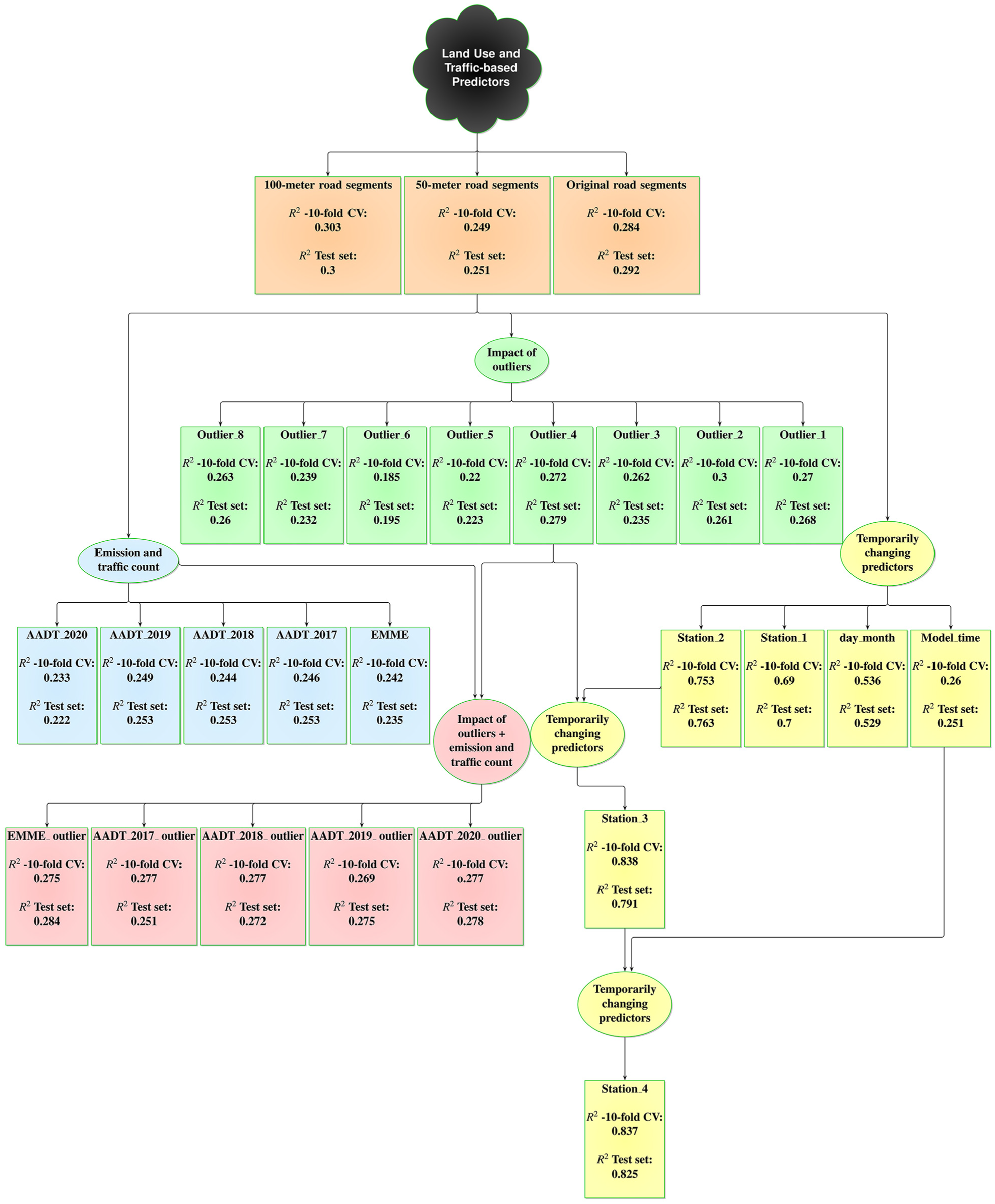
Overview of the 27 models tested for PM2.5 prediction, categorized by data aggregation methods (orange), outlier treatments (green), traffic and emission data impact on models (blue), traffic and emission data impact with outlier treatment (red), and temporally varying predictors (yellow). R2 values are reported for the test set and 10-fold cross-validation (CV).
The two segment aggregation methods (100-m and original segments) were compared with base case to determine their impact on model performance. The 100-m aggregation method performed slightly better than both the 50-m (base case) and the original road segment aggregation for model accuracy. However, the original road segment aggregation, while not as accurate as the 100-m approach, provided more realistic representation of the spatial variability inherent to road networks. These results highlight the importance of testing various spatial aggregation resolutions, as each method balances accuracy with the ability to represent spatial structures and patterns effectively.
We tested the impact of different threshold values for outlier removal on the performance of our XGBoost models for predicting PM2.5 concentration. The threshold values are highlighted in Figure 4a to illustrate the range of data points affected by each outlier removal method. In the first three models (Outlier_1, Outlier_2, and Outlier_3), where we employed outlier removal criteria targeting data points greater than the 99th, 99.7th, and 95th percentiles, the model’s performance exhibited a slight improvement compared with the base case. However, in the third model utilizing the 95th percentile threshold, there is a smaller change in the R2 of the 10-fold CV. This can be the result of removing data points for some days with high concentration that do not qualify as outliers for that day. For the models where we removed datapoints less than the 10th percentile or 20th percentile threshold (Outlier_5 and Outlier_6), the R2 decreased, possibly because correctly recorded data points (not true outliers) may have been removed. As shown in Figure 4, these two methods (removing datapoints less than the 10th percentile or 20th) may result in the removal of most records for some days. In our data, the 5th percentile of the data is equal to zero. For three models, we used the 5th percentile and lower threshold to remove data points. When we just use lower thresholds (Outlier_7 model), the R2 diminished slightly. The results for the Outlier_4 and Outlier_8 models, where we had upper thresholds for 95th and 99.7th percentile, respectively, and zeros were removed, show that the R2 for these two models were slightly better than other ones. However, the model results show that removing outliers does not significantly improve performance in predicting PM2.5 concentrations.
The results of the models that we created by adding local traffic and emission predictors show no improvement, possibly because the impact of traffic had been captured by predictors that we had in the base case model such as road density and road typology.
The results of the models with temporally varying predictors show that by adding day of week and month as predictor, the performance of the model improved significantly. By adding humidity, temperature, and wind speed, the R2 increased from 0.26 to 0.69 which shows the importance of these variables that can capture temporal variability of the model for predicting PM2.5, and by adding concentration of pollutants from stationary stations, the R2 increased to 0.753. Moreover, the results for the Station_3 and Station_4 models demonstrate that by treating outliers and adding weather and regional air quality predictors to the model (Station_2), the performance of LUR models for PM2.5 can be improved substantially.
The best-performing model, Station_4 includes additional features with larger buffer sizes of 500 m, 1000 m, and 2000 m to capture regional impacts. These larger buffers provide a broader spatial context that complements the finer-scale variability captured by smaller buffers, resulting in a balanced representation of both local and regional influences on PM2.5 concentrations. This approach also mitigates concerns about spatial autocorrelation by capturing regional trends and accounting for spatial dependencies in the model. The results of this approach, shown in Figure 7, represent the PM2.5 concentration surface for afternoon hours (3 to 7 p.m.), where the inclusion of larger buffer sizes highlights regional pollution patterns across the study area.
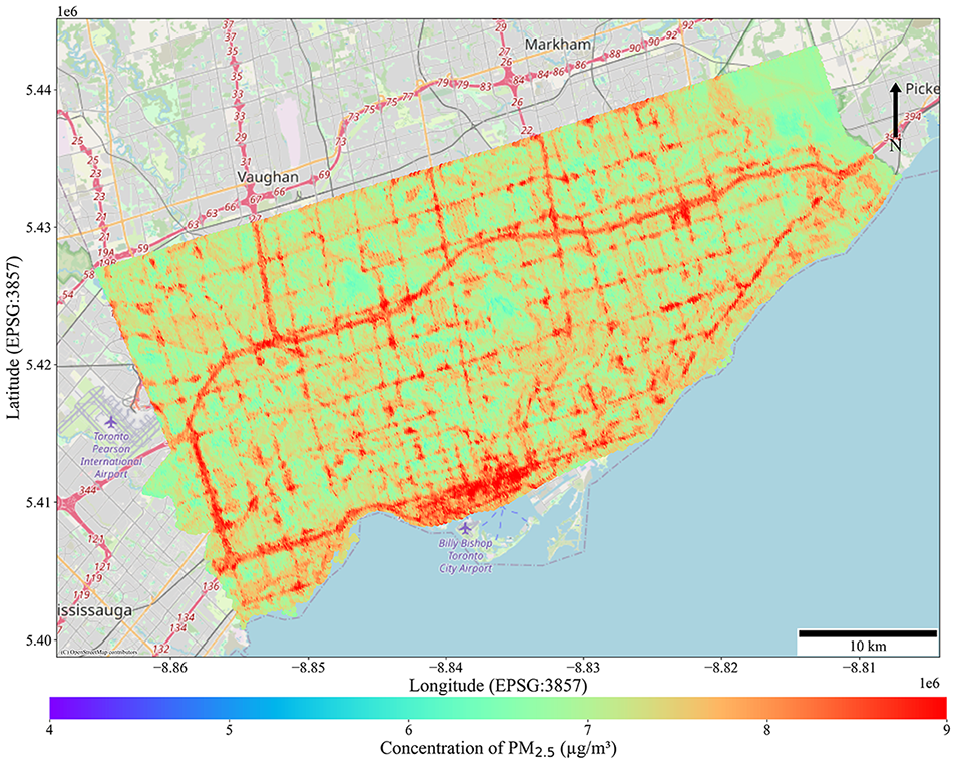
Predicted PM2.5 concentration for the City of Toronto using the Station_4 model during afternoon hours (3 to 7 p.m.).
In Figure 7, the PM2.5 surface using the Station_4 model is used to predict PM2.5 for the entire city, including regions beyond the area that the data was originally collected (beyond downtown area). As expected, higher concentrations are predicted along major roads and highways because of increased emissions. This figure demonstrates that the model effectively predicts pollutant concentrations in locations outside the original data collection area.
Validation Against Observations at Reference Stations
The results of the comparison of the Station_4 model predictions against observations at the four reference stations operated by the Ministry of Environment, Conservation, and Parks are presented in Figure 8. They demonstrate reasonable consistency between the predicted and observed values across different times of day and locations. For instance, in the afternoon, the accuracy of the model’s predictions ranged from 84.6% in Toronto Downtown to 95.5% in Toronto North. Similar patterns were observed during the morning and midday periods, with accuracies exceeding 88% for most comparisons. This consistency highlights the model's ability to extend its predictions beyond the immediate road network, leveraging broad spatial predictors such as land use and meteorology to capture regional trends effectively. While limitations remain in areas far removed from roadways, the updated surface incorporates larger buffer sizes (500 m, 1000 m, and 2000 m), enhancing the model's capability to estimate off-road concentrations more reliably. These findings support the robustness of our approach for predicting spatial pollution patterns across diverse urban areas.
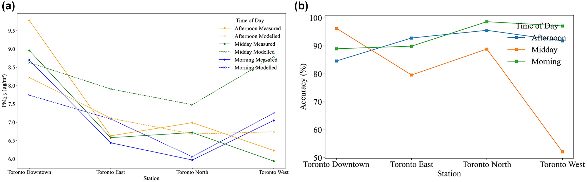
Validation of the Station_4 model against measurements at four regulatory monitoring stations in Toronto. Panel (a) shows the observed (measured) and predicted (modeled) PM2.5 concentrations (in µg/m3) across stations for each time of day (morning, midday, afternoon). Panel (b) presents the calculated accuracy (%) of the model predictions.
Discussion and Conclusion
A mobile monitoring campaign, utilizing a sensor-equipped truck operated by a courier company, demonstrates a novel approach to capture spatiotemporal variations in PM2.5 concentration. The study's timeframe, from June 21, 2022, to January 11, 2023, allows for a nuanced analysis of seasonal influences on air quality. This study investigates factors influencing PM2.5 concentration predictions using LUR models by developing several different models using different sets of predictors. The findings highlight the complex interplay of factors influencing PM2.5 levels, including meteorological conditions, traffic emissions, and land use variables. Considering temporal factors significantly enhanced the model's performance, as evident from the comparison of the day_month model with the base case. The incorporation of day of the week and month as predictors resulted in a substantial improvement in the R2 for both the test set and the 10-fold CV. This improvement suggests that distinct patterns exist throughout the week, possibly influenced by varying human activities, traffic density, and meteorological conditions. Moreover, this improvement suggests that accounting for temporal variations, such as day-of-week patterns and seasonal differences, contributes valuable information to the model. For instance, weekdays might exhibit different pollution patterns compared with weekends, and seasonal variations could be crucial in understanding the impact of weather conditions on PM2.5 concentrations. This finding aligns with previous research emphasizing the impact of temporal variations on air quality and emphasizes the need for comprehensive spatiotemporal models ( 30 , 31 ).
The study also investigated the impact of different spatial aggregation methods on model performance, providing insights into the impact of aggregation method on model prediction. The comparison of three aggregation methods—road segment shapefile, 50-m, and 100-m distanced points—showed that the 100-m resolution performed slightly better than the other points. The results imply that choosing an appropriate spatial aggregation method is crucial for achieving a more accurate representation of local air quality patterns. So, for developing an LUR model, testing several resolutions might help to improve the model’s accuracy which is aligned with the findings of the study by Hankey and Marshall ( 19 ).
The study evaluates the impact of outlier removal on model performance, revealing trade-offs associated with different thresholds. Models that deleted outliers (errors in recording) while retaining non-outlier records demonstrated improvement in the performance compared with models with extensive data removal. For instance, the Outlier_4 model, which focused on removing data greater than the 95th percentile while keeping lower concentrations, exhibited a slightly better R2 for both the test set and 10-fold CV. This indicates that careful outlier handling, preserving valid data points, contributes to a more robust and accurate LUR model as has been shown in previous studies ( 32 , 33 ). However, this study shows that it is essential to strike a balance, as overly aggressive outlier removal may lead to the loss of crucial information and compromise model performance.
The inclusion of predictors related to emissions and traffic counts presented mixed results. While the addition of predictors from EMME and AADT data did not show significant improvement in the base case model, it is crucial to note that the base case model already included relevant predictors related to land use, traffic, and location. The lack of substantial improvement suggests that the existing set of predictors in the base case model adequately captured the spatial variability caused by traffic and emissions in PM2.5 concentrations. This finding underscores the importance of carefully selecting predictors based on the study context and existing knowledge of local sources of pollution.
The models incorporating data from stationary monitoring stations as predictors exhibited a remarkable increase in performance. The introduction of temporal predictors, such as time of day and month, as well as data from stationary monitoring stations, enhances the ability of models to capture temporal variation. The marked improvement in R2 values for models incorporating temporal variables highlights the significance of considering time-related factors in predicting PM2.5 concentrations.
In this study, we relied on cross-validation to evaluate our models’ performance because of the limited availability of independent data for validation. While this approach provides a useful measure of model accuracy, we acknowledge that random cross-validation can potentially result in overfitting, especially when using datasets with limited spatial diversity. Future research should aim to include independent datasets or temporal validation to further test the robustness of the model and ensure its transferability across space.
In conclusion, this analysis shows that taking temporal, spatial, and outlier-related factors into account can help develop accurate LUR models for predicting PM2.5 concentrations. The results show that the integration of innovative monitoring techniques, thoughtful predictor selection, and exploration of outlier impact could be used to improve LUR model accuracy. Our findings underscore the need for a multidimensional approach that considers both spatial and temporal factors to enhance the accuracy of models for PM2.5 concentrations.
Footnotes
Author Contributions
The authors confirm contribution to the paper as follows: study conception and design: Junshi Xu, Marianne Hatzopoulou, Matthew Roorda; data collection: Milad Saeedi, Junshi Xu, Usman Ahmed; analysis and interpretation of results: Milad Saeedi, Marianne Hatzopoulou; draft manuscript preparation: Milad Saeedi, Marianne Hatzopoulou, Matthew Roorda. All authors reviewed the results and approved the final version of the manuscript.
Declaration of Conflicting Interests
The author(s) declared no potential conflicts of interest with respect to the research, authorship, and/or publication of this article.
Funding
The author(s) disclosed receipt of the following financial support for the research, authorship, and/or publication of this article: Funding for this project was provided by the Natural Sciences and Engineering Research Council of Canada (NSERC) under grant ALLRP 555620 - 20 (“City Logistics for the Urban Economy”), Purolator Inc., Geotab, and the City of Toronto.