
Abstract
The macroscopic fundamental diagram (MFD) is an effective model for monitoring, predicting, and controlling urban traffic. A critical factor in accurately observing an empirical MFD is the spatial homogeneity of traffic states, which can be achieved through effective clustering of urban networks. This study explores and compares various machine learning (ML) clustering algorithms, including k-means, Gaussian mixture models (GMM), density-based spatial clustering of applications with noise (DBSCAN), and hierarchical agglomerative clustering (HAC), to enhance traffic homogeneity and spatial connectivity. Our methodology evaluates these algorithms using traffic-relevant indicators such as homogeneity, connectivity, MFD shape, and travel time estimation accuracy, contrasting them with clustering methods from the literature, such as snake similarity and sensor-bias-corrected community detection (SBCCD). The results demonstrate that ML algorithms, especially when optimized for hyperparameters, consistently surpass state-of-the-art methods in computational performance and, in most cases, achieve a good balance between homogeneity and connectivity of the resulting clusters. Specifically, GMM produces highly homogeneous clusters ideal for routing and macroscopic travel time estimation, although they lack connectivity. In contrast, HAC ensures connected clusters suitable for traffic management strategies such as perimeter control and congestion pricing. k-means achieve a balanced performance between homogeneity and connectivity, while DBSCAN effectively identifies congestion pockets that may interest transport planners. These findings highlight ML algorithms as promising alternatives to more complex methods.
Keywords
In analogy to the traffic fundamental diagram (FD) at the link level, Daganzo ( 1 ) and Geroliminis and Daganzo ( 2 , 3 ) have demonstrated the existence of a relationship between the average flow and the average density at the network level, known as the macroscopic fundamental diagram (MFD) or the network fundamental diagram (NFD). The MFD can be approximated analytically ( 4 – 7 ) or measured empirically ( 8 – 10 ). The analytical approximation is valid only for arterial roads without any net turning flows at intersections, or for symmetrical grid networks that can be approximated as arterials. The corresponding MFD is therefore considered independent of demand and influenced solely by supply-related characteristics. As such, the analytical MFD represents the upper bound of traffic performance, observable under regularity conditions, characterized by slowly varying and well-distributed demand. However, real networks are rarely homogeneous and turning flows do affect congestion patterns. Consequently, empirical MFDs are clearly demand-dependent and are particularly influenced by the spatial and temporal distribution of vehicles within the network, as demonstrated, for example, by the hysteresis phenomenon.
Many studies have been devoted to understanding the effect of relaxing the regularity conditions, specifically the heterogeneous spatial distribution of traffic density ( 8 , 11 – 13 ). It has been shown that travel demand ( 14 – 17 ), road topology ( 8 , 18 , 19 ), control strategies ( 17 , 20 ), and route choice ( 5 , 21 ) significantly affect the spatial distribution of traffic density and, therefore, the shape of the MFD.
The MFD provides a basis for efficiently modeling, monitoring, and controlling urban traffic at a low computational cost. As a result, MFD-based traffic management and control applications have gained increasing attention in research. These include perimeter control ( 22 ), macroscopic route guidance ( 21 ), parking management ( 23 ), mobility pricing ( 24 , 25 ), and road space allocation ( 26 ). The fundamental idea behind many MFD applications is to monitor and predict traffic conditions at the regional level under certain constraints, and to react accordingly to maintain traffic densities within a favorable range. However, MFD scatter or hysteresis can reduce the accuracy of traffic state predictions. If the traffic state in a network cannot be predicted accurately, the quality of control based on these predictions will consequently decrease. Therefore, identifying homogeneous regions within the network is crucial to observing a well-defined MFD and ultimately improving the effectiveness of MFD-based applications. Several clustering algorithms have been proposed in the literature for this purpose.
The remainder of this paper is organized as follows. The literature review section outlines the recent state of the art and presents the contribution of this work. The methodology section describes the approach used in our comparative analysis, including the algorithms evaluated. The case studies that form the basis of the analysis are introduced in the case studies section. This is followed by a presentation and interpretation of the results in the results section. Finally, we conclude with a discussion of the implications of our findings in the practical applicability and generalizability and Conclusion sections.
Literature Review
The main goal of any clustering method is to group urban network links based on an underlying measure of similarity to facilitate future applications. A crucial consideration is how to effectively cluster urban networks into regional sub-networks. Ideally, the partitioned regions should balance several factors: they should be of similar size, topologically connected, compact, and well separated. At the same time, traffic conditions within each region should be relatively homogeneous to reduce MFD scatter or hysteresis. These objectives can often be contradictory, requiring trade-offs. Different MFD applications may prioritize one objective over another, depending on their specific needs and goals.
For routing applications and fleet control, it is important that the traffic state within each cluster is homogeneous ( 27 – 29 ). For multi-reservoir MFD modeling, the compactness and connectivity of each region are crucial ( 30 ); although not strictly required, these properties also simplify the estimation of the region’s average trip length ( 31 ). When congestion propagation is modeled with reaction–diffusion methods, partitioning the urban road network into regions that share similar congestion dynamics enables accurate modeling ( 32 ). Finally, for perimeter-control strategies, compact and well-connected regions are again essential ( 33 ).
Various researchers have explored different methodologies for partitioning urban networks for MFD applications. Ji and Geroliminis ( 34 ) proposed a static method involving: (i) initial segmentation based on Gaussian kernel similarity and the normalized cut algorithm, (ii) merging, and (iii) boundary adjustment. While foundational, this method was tested on a symmetric network and did not account for directional flows or similarities between adjacent links. Saeedmanesh and Geroliminis ( 35 ) developed a static clustering approach using “snake” similarities, which, despite capturing spatial correlations, is computationally intensive, particularly for large-scale networks. An et al. ( 36 ) suggested a static methodology combining lambda-connectedness and region-growing segmentation, requiring minimal input data. Nonetheless, uneven cluster sizes affected MFD estimation. Ambühl et al. ( 37 ) proposed a Monte-Carlo-like partitioning method based on community detection and random-walk search to generate homogeneous and connected partitions using stationary sensor data. Batista et al. ( 38 ) employed Gaussian mixture models (GMM) for static clustering based on topological characteristics, resulting in connected clusters; however, the homogeneity of the resulting clusters was not examined.
Incorporating the temporal dimension and thereby accounting for the dynamic aspect of urban traffic, Zhou et al. ( 39 ) proposed a method to calculate the correlation between adjacent intersections, considering both physical features and dynamic traffic measurements. They then employed a community detection method to cluster the network. Although the method produced homogeneous, connected, and compact regions, it was tested only on a synthetic grid-type network. Ji et al. ( 40 ) utilized the concept of maximum connected components from graph theory to dynamically identify congested parts of the network, providing insights into congestion propagation, but encountered practical challenges in perimeter control owing to non-compact cluster borders. Pascale et al. ( 41 ) proposed a dynamic method that extends ( 34 ) by incorporating time-dependent density measurements and refining similarity estimation. Rempe and Bogenberger ( 42 ) applied clustering to extract congestion-prone regions, analyzed their correlations, and utilized this analysis to formulate a k-nearest neighbors (KNN) predictor for estimating travel time losses. Saeedmanesh and Geroliminis ( 43 ) further extended their snake method to include the temporal dimension, ensuring high connectivity and homogeneity, albeit at a high computational cost, thereby raising questions about its practical feasibility. Lopez et al. ( 44 ) compared various clustering methods using speed measurements from travel time data, finding k-means marginally superior. This was tested on an abstract representation of Amsterdam’s road network. Casadei et al. ( 45 ) developed a graph theory-based clustering method for urban networks, in which nodes are clustered if connected by paths meeting specific criteria related to road type and speed. Clusters are formed by removing non-conforming edges and identifying weakly connected components. This method yielded connected paths rather than compact regions. Bellocchi et al. ( 46 ) proposed a dynamical efficiency measure in multimodal multilayer networks that detects evolving congestion clusters and critical intermodal junctions, enhancing understanding of urban traffic dynamics. Jiang et al. ( 47 ) explored partitioning urban networks with polycentric congestion patterns. Their dynamic method involves a six-step algorithm for partitioning large-scale urban networks through the integration of traffic data and geographic connectivity. This process includes graph definition, data pre-processing, feature handling, identification of clusters and partitions, and boundary reshaping.
The list of papers earlier demonstrates the significant interest in the clustering of urban networks within the research community. However, it is well established that no single method is optimal for clustering urban networks, which justifies the diversity of existing approaches ( 48 ). Most of these methods focus on clustering based on graph theory and involve complex estimations of similarity between each pair of links within the network. These approaches can be computationally intensive, a constraint that becomes more pronounced as the network size increases. The goal of this study is to compare multiple clustering algorithms and methods to evaluate the trade-offs between traffic homogeneity, spatial connectivity, and computational cost for practice-relevant applications such as route guidance and perimeter control. In pursuing this goal and addressing the related research gap, the present work makes the following contributions to the state of research:
We compare machine learning (ML) clustering algorithms and other state-of-the-art methods to assess trade-offs between traffic homogeneity, spatial connectivity, travel time estimation accuracy, and computational cost for specific practice-relevant applications.
We conduct the comparison using calibrated traffic simulations based on real networks to enhance the practical relevance of our study.
We perform the study on different networks to mitigate case-specific effects and increase the generality of our conclusions.
Methodology
As stated earlier, the goal of this study is to compare ML clustering algorithms and other state-of-the-art methods. ML clustering algorithms vary in their mathematical formulation, hyperparameters, and computational complexity. Accordingly, the quality of results for applications varies, and the appropriate clustering algorithm for a specific application often needs to be selected experimentally ( 49 ). Therefore, we apply different ML algorithms to the network clustering problem. The focus is on clustering algorithms that use Euclidean distance as a measure of similarity between data points. Owing to their simplicity and computational efficiency, such algorithms are well suited for large-scale and real-time applications.
Building on this foundation, within the proposed methodological framework for clustering urban networks, the algorithms evaluated include k-means, GMM, density-based spatial clustering of applications with noise (DBSCAN), and hierarchical agglomerative clustering (HAC). The schematic illustration in Figure 1 outlines the process, beginning with the collection of static link attributes and traffic data from a simulation scenario. This is followed by the optimization of clustering hyperparameters and feature weights to achieve optimal clustering results. The performance of these algorithms is assessed using a set of traffic-relevant indicators that reflect the objectives of the clustering process, namely homogeneity, connectivity, and travel time estimation accuracy. The ML algorithms are compared against state-of-the-art methods, primarily the snake similarity and sensor-bias-corrected community detection (SBCCD). The following sections introduce the performance indicators, detail the formulation of the clustering problem, describe the solution algorithm, and outline the implementation procedure.
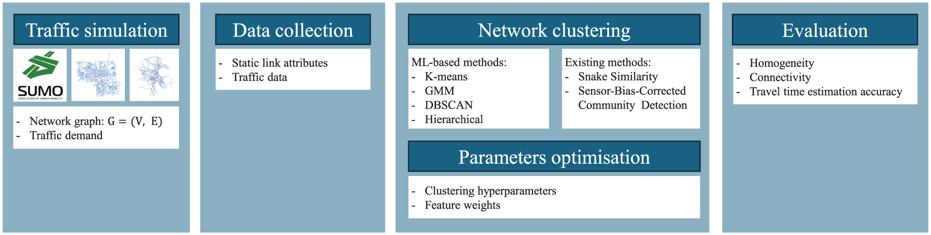
Schematic illustration of utilised methods.
Performance Indicators
The quality of the clustering results is evaluated using indicators in three categories, reflecting the main objectives of creating homogeneous, connected clusters that facilitate MFD-based applications.
Homogeneity
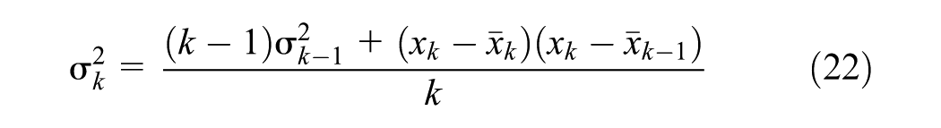
Homogeneity is assessed using two indicators. First, the normalized total variance, which is defined as the ratio of the total within-cluster variance to the global variance of the network. To account for cluster size, the variance of each cluster is weighted by its length. The formula for (

where
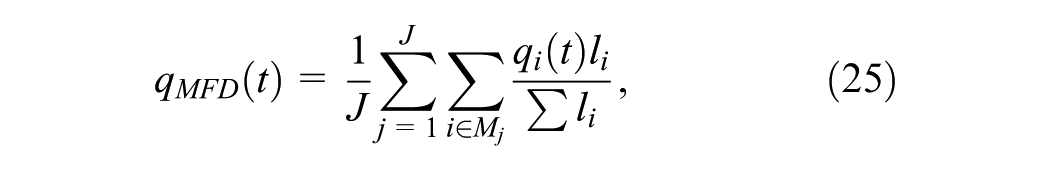
Second, the scatter of the MFD is quantitatively evaluated. The MFD is estimated by averaging link flows,


The area covered by the MFD points is used as an indicator of the scatter of the MFD, reflecting the heterogeneity within the subnetwork. The smaller the area, the more homogeneous the subnetwork’s traffic state is. To achieve this,
Connectivity
Connectivity is quantified using the indicator

Accuracy of Travel Time Estimation
Finally, homogeneous clustering implies that the links within a cluster exhibit similar speeds that are close to the cluster’s average speed. This can be useful for estimating travel times of trips completed within the network while maintaining high computational efficiency.
Given a trip from link

where
For a representative number of trips, the resulting margin of error in travel time estimation reflects the homogeneity of the clusters. The more homogeneous a cluster is, the closer the link speeds are to the cluster’s average speed, and the more accurate the travel time estimation becomes.
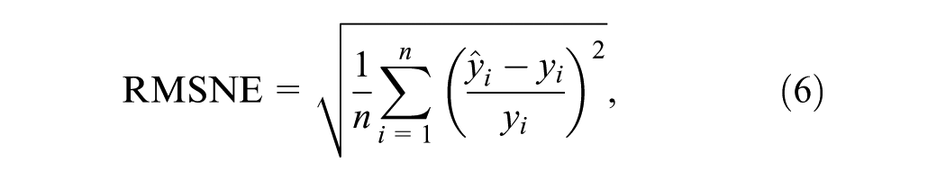
We evaluate the accuracy of the travel time estimation using a sample of trips completed in the simulation scenario. The sample size is set to 75% of all trips completed in the network and is randomly selected at each evaluation time. Estimated travel times are then compared with actual travel times obtained from the simulation. The error function used to assess accuracy is the root mean squared normalized error (RMSNE), which calculates the average of the squared relative errors between the estimated and actual travel times, as defined in Equation 6.
where
Machine Learning Clustering Algorithms
Features Vector Extraction
The input to the ML algorithms is a vector space, where each link in the network is represented by a vector comprising multiple features that describe the link’s attributes and traffic state. Thus, the entire input space can be represented as an
In this study, we selected as features the

When an adaptive signal controller is present, practitioners may wish to let the clustering sense its homogenizing effect by adding control-aware features. In our framework this is straightforward: simply extend each link’s feature vector with one or more control-sensitive terms, for example the green ratio
If adaptive-control data are unavailable, the original three-dimensional vector
Parameters Fine-tuning
ML algorithms often require specific hyperparameters as input. For example, many clustering algorithms need the number of clusters

where
The weights
k-Means
Owing to its simplicity and efficiency, k-means is one of the most widely used clustering algorithms for scientific and industrial applications. Given a data set
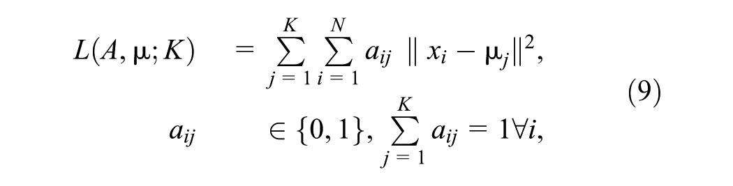
where
Finding the exact global minimum of Equation 9 is NP-hard. k-means therefore alternates two steps until convergence (
50
,
52
). The algorithm starts with
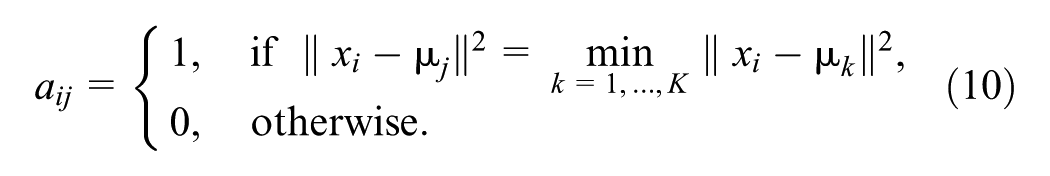

Because
Gaussian Mixture Model
The GMM is a soft probabilistic clustering method. It assumes that a data set can be represented as a mixture of parameterized multivariate Gaussian distributions, each corresponding to a cluster. Given a data set
where the mixing coefficients
The objective is to find the parameter set
Optimization challenges primarily arise from the logarithm of the sum inside Equation 13. To simplify the optimization, latent variables
Because
EM increases the log-likelihood monotonically until convergence to a local maximum. It is sensitive to the starting values of
Density-Based Spatial Clustering of Applications with Noise
DBSCAN partitions the data set into contiguous dense regions (clusters) separated by sparse regions. The standard DBSCAN algorithm proposed by Ester et al. (
56
) characterizes dense versus sparse regions by means of two input parameters: neighborhood radius,

where
If the -neighborhood of a point
The algorithm starts with an arbitrary point
Ester et al. (
56
) suggest using the
Hierarchical Agglomerative Clustering
HAC builds a hierarchy of clusters by iteratively merging the pair of clusters with the smallest distance. Given a data set
where
HAC can also incorporate connectivity constraints that restrict merging to spatially adjacent clusters. This modification is expressed by Equation 21.
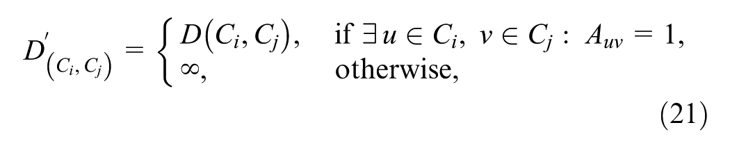
where
The connectivity constraints are particularly useful for clustering geographical objects, for example, segments of a road network, because they ensure that only spatially contiguous clusters are merged.
State-of-the-art Clustering Methods
Snake Similarity
The snake method was initially introduced in Saeedmanesh and Geroliminis (
35
). In this method, each link in the network initiates a sequence termed a “snake” by iteratively adding one adjacent link to the current sequence of links that minimizes the variance of the sequence’s properties, such as traffic flow or density. The formulas for variance,

These snakes are then used to estimate the similarity between link pairs in the network. The similarity metric,
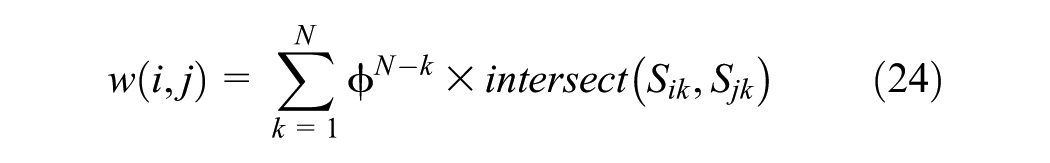
In this equation,
For this study,
Sensor-Bias-Corrected Community Detection
The SBCCD method introduced by Ambühl et al. ( 37 ) is a two-step process to partition urban traffic networks into homogeneous regions and accurately estimate MFDs. Unlike other methods studied, this approach inherently requires less data by relying solely on stationary sensor data. First, multiple candidate partitions are generated based on the network’s topology using a community detection algorithm based on random walks, ensuring that each region is geographically contiguous and connected. Second, for each candidate partition, MFDs are estimated using a re-sampling method with a correction applied to account for sensor placement biases along the links, as detailed in Equations 25 and 26.
where
The heterogeneity measure

where
Case Studies
The first case study is a microscopic simulation model of Ingolstadt, Germany, covering an area of approximately 10 km by 10 km, Figure 2b. The road network, traffic control system, and traffic demand were modeled and calibrated in Simulation of Urban MObility (SUMO) software ( 61 , 62 ). The network extends for 1,248 km-ln and comprises around 12,000 links connected via 5,600 intersections. Speed limits across the network range from 20 km/h to 120 km/h, depending on the road category. All traffic signals in the network are modeled as multi-phase, fixed-time controlled. However, the impact of adaptive traffic signal control is still considered by averaging green time adaptations and setting a specific traffic light program for each signal on an hourly basis. The demand in the simulation is defined as time-dependent vehicle routes, with a 20% probability of route adaptation based on traffic conditions.
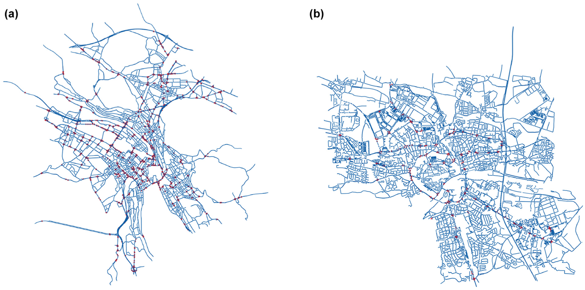
Case studies. (a) Zurich network. (b) Ingolstadt network.
The second case study is a mesoscopic simulation model of Zurich, Switzerland, covering an area of approximately 13 km by 14 km, Figure 2a. The road network, traffic control system, and traffic demand were modeled and calibrated in SUMO. The network extends for 980 km-ln and comprises around 7,240 links connected via 3,530 intersections. Roads are split into 100 m segments, with traffic dynamics modeled on a segment-to-segment basis. These dynamics are constrained by link capacities and vehicles’ desired headways, allowing for realistic modeling of vehicle queues and individual vehicle movements. Traffic signal timings are defined uniquely for each intersection. For a typical intersection, the cycle time is set to 48 s and the green time to 16 s. These values are based on interviews with local operators. Intersection delays were scaled by a factor of 0.5 to account for intersection capacity and the average level of signal coordination. The time-dependent traffic demand is estimated using an endogenous procedure based on one year of data from loop detectors. Vehicles are periodically stochastically routed based on the current traffic state of the network. On entering the network, vehicles are assigned to a stochastic shortest path, with link speeds overestimated by a uniformly distributed random factor between 1 and 1.8.
Both simulation scenarios include a mix of urban and highway roads, featuring varying lane counts and speed limits. The networks exhibit an irregular topology (asymmetric structure) with hierarchical components and varying levels of spatial connectivity. The defined traffic demand results in different spatial and temporal congestion levels, directly influencing the observability and shape of the MFD, which makes the application of the methodology more challenging. A 24 h simulation period is used, with lane density and space-mean speed recorded every 5 min, a duration sufficient to comprise a few traffic signal cycles. Flow is estimated using the identity
Results
The methodological framework is implemented in Python using the sklearn package (
63
). We begin by examining the effects of
Effect of weights in the objective function.
The clustering process begins with fine-tuning the hyperparameters, specifically the number of clusters,
Figure 4 presents the fine-tuning results for k-means clustering applied to the Zurich network. Figure 4a shows the objective value, computed as described in Equation 8, plotted against the number of clusters. As the number of clusters increases, the objective value initially increases, reflecting improved clustering performance through a better balance of homogeneity and connectivity. However, beyond a certain point, the curve flattens, indicating diminishing returns in performance gains. For a given traffic weight, the objective value generally remains within the same order of magnitude, suggesting that the traffic feature weight sets a baseline for clustering performance, with the number of clusters fine-tuning the results.
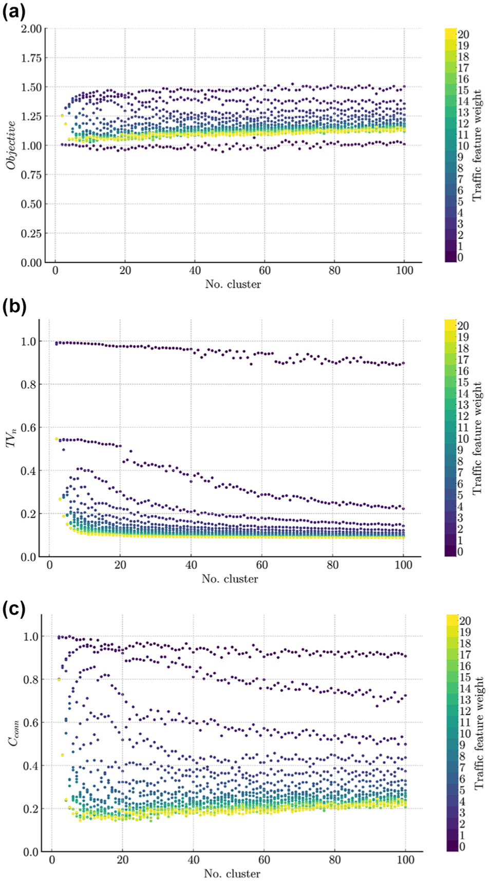
k-means fine-tuning for Zurich network. (a) Objective evaluation. (b) TVn evaluation. (c) Cconn evaluation.Note: TVn = normalized total variance; Cconn = connectivity indicator.
Interestingly, neither higher (brighter shades) nor lower (darker shades) density weights alone guarantee optimal performance. Instead, achieving a balance between homogeneity and connectivity is crucial. However, doubling the density weight achieves an optimal trade-off, improving connectivity and reducing variance without causing excessive cluster fragmentation.
Figure 4b examines
Figure 4c focuses on
Given the size of the networks and after empirical assessment, the number of clusters is capped at a maximum of 15. Taking Zurich as an example, Figure 4a shows that increasing the number of clusters beyond this point provides only marginal improvements in the combined objective value of homogeneity and connectivity. Moreover, it is not practically feasible to have many clusters with many state variables, as this increases the computational complexity of the modeling, making it harder to apply real-time traffic control. For each scenario, the number of clusters range from 2 to 15, while the density weight ranges from 1 to 10, resulting in a total of 117 configurations for each scenario and method. The coordinate weight is fixed at 1. This method of choosing hyperparameters allows easy tailoring of the clustering outcome to the specific requirements of the application. Feature weights and hyperparameters can be varied within different ranges, or weighting factors can be introduced in Equation 8 to assign greater importance to connectivity or homogeneity. The results of ML algorithm fine-tuning are illustrated in Table 1.
Parameters After Hyper-Parameter Optimization
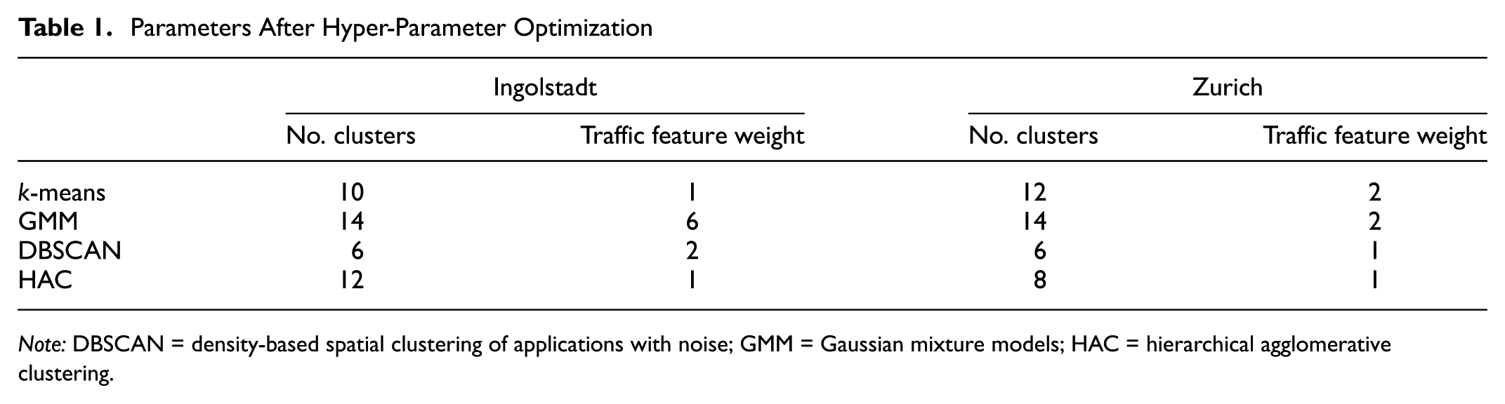
Note: DBSCAN = density-based spatial clustering of applications with noise; GMM = Gaussian mixture models; HAC = hierarchical agglomerative clustering.
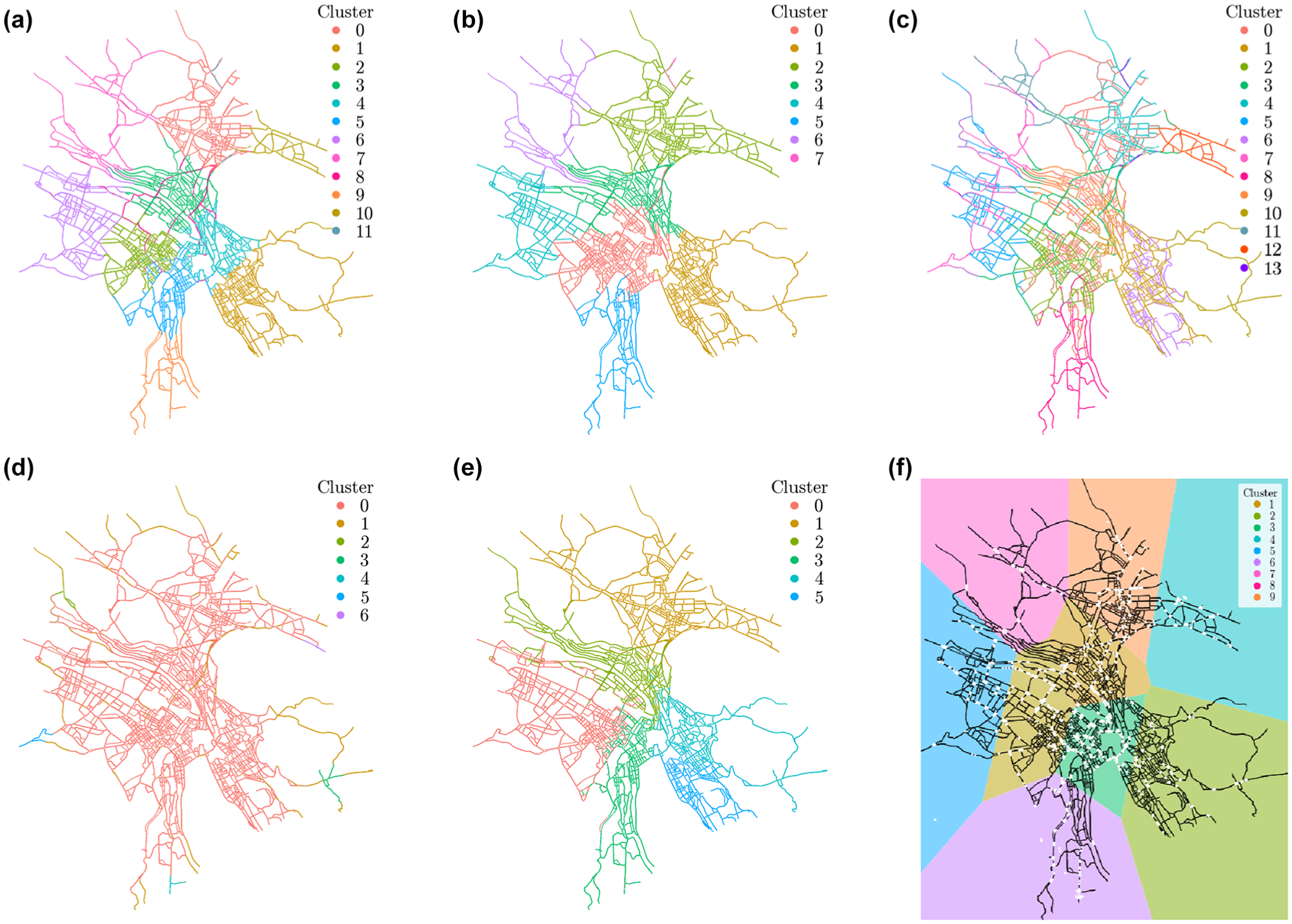
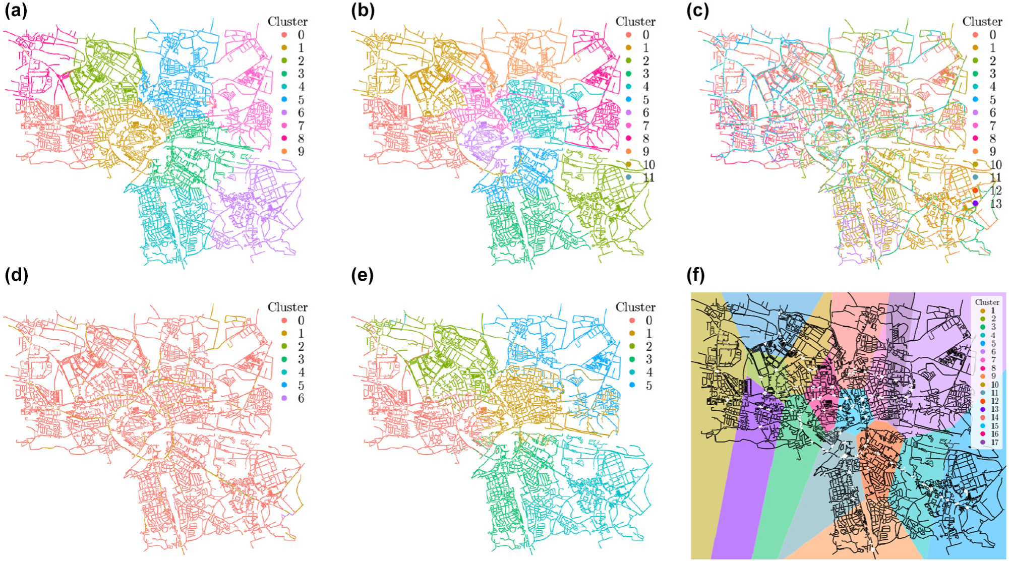
Based on the fine-tuned parameters in Table 1, Figures 5 and 6 illustrate the clustering results for Zurich and Ingolstadt, respectively. The clusters are distinguished by different colors, as shown in the respective legends. For Zurich, k-means and HAC identify distinct regions, while the GMM clustering outcomes appear to align with major traffic corridors. In contrast, the DBSCAN results tend to be fragmented and uneven in size, highlighting localized density variations. Similar patterns are observed for Ingolstadt; however, the results are also influenced by the network topology.
Zurich clustering results. (a) k-means. (b) hierarchical agglomerative clustering (HAC). (c) Gaussian mixture models (GMM). (d) density-based spatial clustering of applications with noise (DBSCAN). (e) snake similarity. (f) sensor-bias-corrected community detection (SBCCD).
Ingolstadt clustering results. (a) k-means. (b) hierarchical agglomerative clustering (HAC). (c) Gaussian mixture models (GMM). (d) density-based spatial clustering of applications with noise (DBSCAN). (e) snake similarity. (f) sensor-bias-corrected community detection (SBCCD).
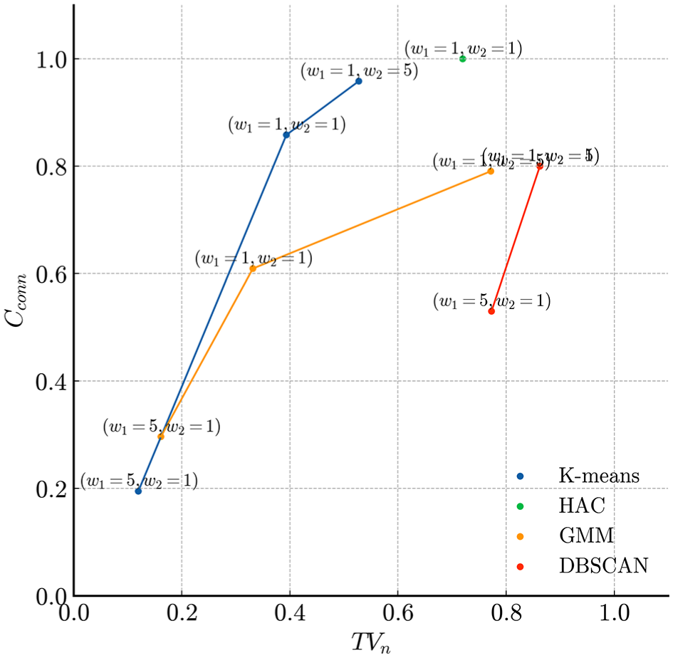
Table 2 summarizes the indicators used to evaluate the clustering outcomes. In both cities, GMM and k-means show the best performance in regard to
Overview of Study Indicators (↑ Preferred when Higher; ↓ Preferred when Lower)
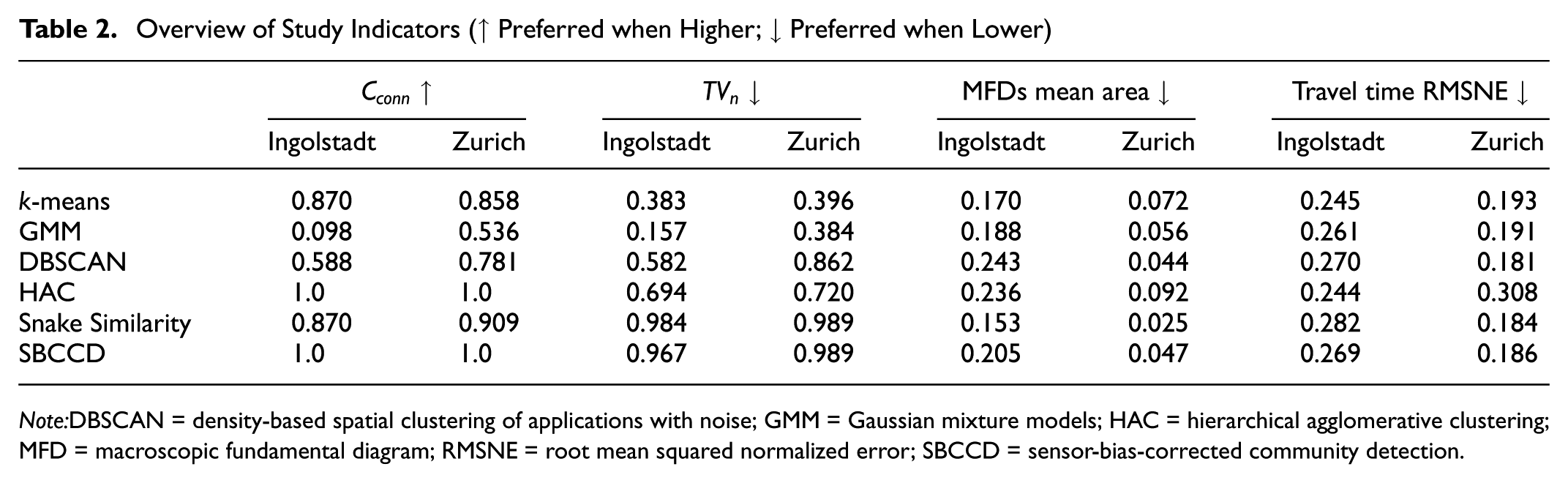
Note:DBSCAN = density-based spatial clustering of applications with noise; GMM = Gaussian mixture models; HAC = hierarchical agglomerative clustering; MFD = macroscopic fundamental diagram; RMSNE = root mean squared normalized error; SBCCD = sensor-bias-corrected community detection.
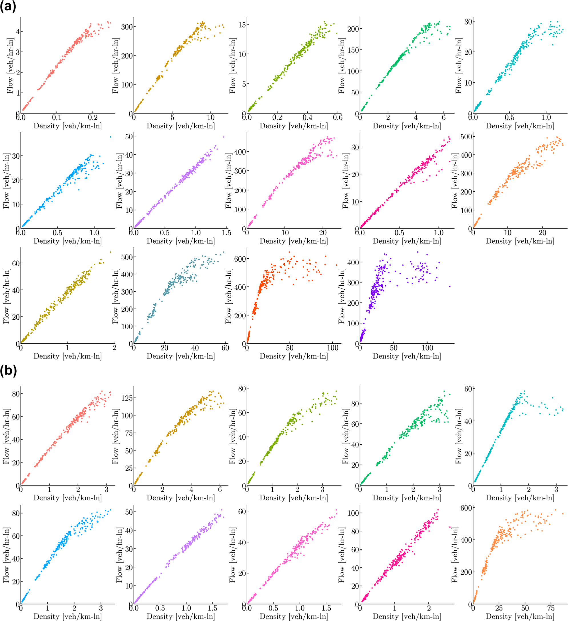
Comparative macroscopic fundamental diagrams (MFDs) for Ingolstadt. (a) Ingolstadt MFDs based on Gaussian mixture models (GMM) clusters. (b) Ingolstadt MFDs based on k-means clusters.
Although k-means and GMM show very similar performance in
With explicit connectivity constraints, HAC always guarantees connected clusters, where any link in a cluster can be reached from any other link. Nonetheless, this affects homogeneity, with
After estimating the similarity matrix, the number of clusters for the snake similarity method is determined using Equation 8 by varying the number of clusters. Although the snake similarity produces clusters that are nearly connected, the
For the SBCCD method, clustering is performed based on the outcomes of virtual sensors in the simulation, where the sensor locations correspond to the actual positions of loop detectors in the real network. However, the evaluation is based on the full information from the simulation. Similar to HAC, this method results in connected clusters, but with a higher
Concerning travel time estimation error, all methods exhibit relatively similar performance. One possible explanation is that the errors in travel time estimation on individual links cancel out, resulting in the total travel time at the end of the trip being very close to the actual travel time. This suggests that the estimation of travel time may be insensitive to smaller variations in traffic state variance.
Additionally, while the estimate of
Generally, computationally efficient algorithms optimize resource usage, enabling faster, scalable, and cost-effective applications. ML algorithms have shown the best performance in this regard, with run times between 1 and 2 s for both cities. On the other hand, the snake similarity, despite producing homogeneous results, is extremely costly in regard to computational resources, taking 234,000 s (approximately 2.7 days) for Ingolstadt and 43,100 s (approximately 0.5 days) for Zurich. SBCCD has moderate run times of 4,080 s for Ingolstadt and 7,500 s for Zurich, balancing performance and efficiency. For static clustering performed offline or at low frequencies, computational efficiency may not be a significant concern. However, congestion patterns can change rapidly within short time frames. To capture these dynamic patterns effectively, time-dynamic clustering with efficient computation becomes essential. In such cases, repeating a static clustering method at each time interval could be a viable solution, though it comes with increased computational demands. Many MFD-based real-time applications operate on control cycles of 3–5 min, requiring updated clustering results within each cycle to respond to evolving traffic conditions ( 47 ). Efficient algorithms ensure that these updates can be performed within the limited time available.
Additionally, the scalability of these algorithms becomes evident when considering the network sizes: Ingolstadt’s network consists of approximately 12,000 links, while Zurich’s has 7,240 links. Despite the larger size of Ingolstadt’s network, ML algorithms maintain low computational times, demonstrating their scalability in handling larger data sets efficiently. In contrast, the snake method’s computational time increases significantly with network size, limiting its practicality for large-scale applications.
Practical Applicability and Generalizability
Table 3 condenses the quantitative findings from the Results Section into a practitioner-oriented matrix. Scores for homogeneity (
Algorithm Suitability Matrix
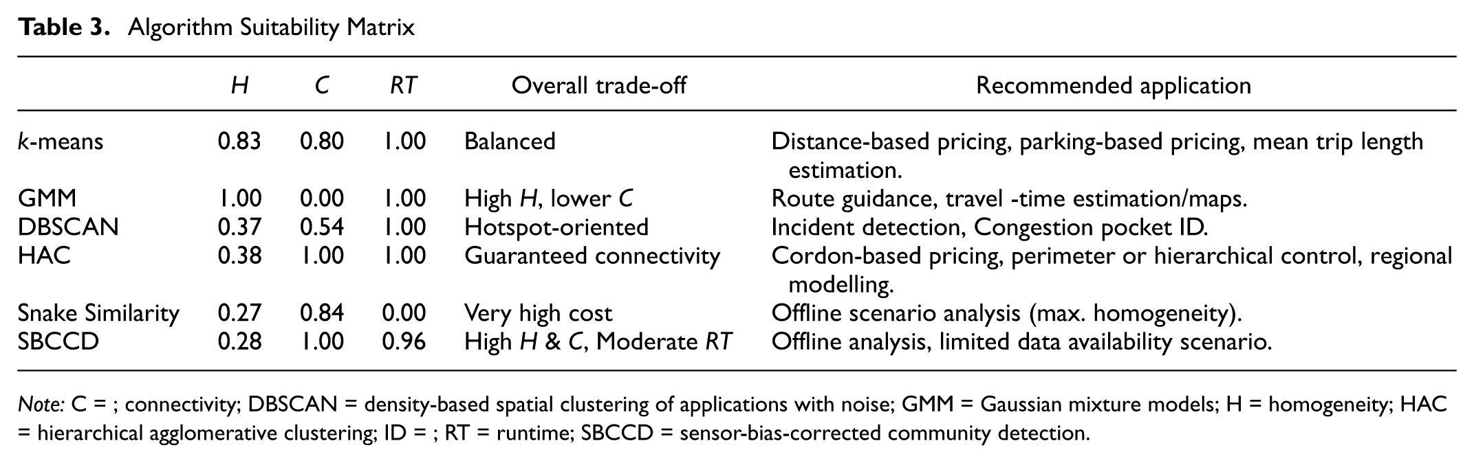
Note: C = ; connectivity; DBSCAN = density-based spatial clustering of applications with noise; GMM = Gaussian mixture models; H = homogeneity; HAC = hierarchical agglomerative clustering; ID = ; RT = runtime; SBCCD = sensor-bias-corrected community detection.
GMM, which achieves the highest
Although Zurich and Ingolstadt differ considerably in size and network density, both are compact European cities with strong public-transport orientations. For networks that deviate more markedly from our case studies, we believe two factors become decisive:
Practitioners are therefore advised to (i) select features appropriate to their specific problem and data availability, (ii) fine-tune hyperparameters and feature weights, and (iii) calibrate
Conclusion
This paper contributes to the literature on urban network clustering by providing a comparative analysis of ML clustering algorithms. Our study assesses the trade-offs among traffic homogeneity, spatial connectivity, and computational cost for practical applications. To ensure the study’s relevance, we conduct this comparison on real networks with calibrated traffic simulations. This approach helps mitigate case-specific effects and strengthens the overall conclusions.
The results show that ML algorithms emerge as promising alternatives to the more complex methods found in the literature because of their performance and efficiency. We apply these ML algorithms to two different networks and observe varied performance in regard to homogeneity and connectivity. Specifically, GMM produces highly homogeneous clusters, making it suitable for routing and macroscopic travel time estimation, yet its clusters are often not well connected or compact. In contrast, HAC with connectivity constraints ensures the formation of connected clusters, which benefits traffic management schemes such as parameter control and congestion pricing. k-means demonstrates balanced performance between homogeneity and connectivity. Although DBSCAN does not perform well on these indicators, it effectively highlights congestion pockets that may warrant further investigation by transport planners.
These insights are likely to hold in cities whose network descriptors fall within the ranges examined here; nonetheless, networks with strongly divergent topologies should first re-tune the homogeneity–connectivity parameters and verify stability through a sensitivity analysis. Extending the empirical validation to grid-based and polycentric networks is a key direction for future work. Future work could also focus on validating these findings with empirical traffic data to enhance their practical relevance. This includes exploring scenarios with limited data availability, such as those relying on loop detectors with limited spatial coverage. Finally, future studies should incorporate the temporal dimension of traffic dynamics, develop post-processing algorithms that correct connectivity and adjust cluster boundaries, and refine performance indicators, particularly the mean area of MFDs.
We make the program code used in this study publicly available at: https://github.com/alayasreih/NetworkClustering.
Footnotes
Acknowledgements
The authors acknowledge Transcality AG for sharing a calibrated simulation model of Zurich for research purposes. We also thank Lukas Ambühl for providing the code for the Sensor-Bias-Corrected Community Detection clustering method.
Author Contributions
The authors confirm contribution to the paper as follows: study conception and design: Y. Alayasreih, G. Tilg, F. Dandl, M. Keyvan-Ekbatani, K. Bogenberger; data collection: Y. Alayasreih, G. Tilg; analysis and interpretation of results: Y. Alayasreih, G. Tilg, F. Dandl; draft manuscript preparation: Y. Alayasreih, G. Tilg, F. Dandl. All authors reviewed the results and approved the final version of the manuscript.
Declaration of Conflicting Interests
The authors declared no potential conflicts of interest with respect to the research, authorship, and/or publication of this article.
Funding
The authors disclosed receipt of the following financial support for the research, authorship, and/or publication of this article: Yamam Alayasreih acknowledges funding by the German Federal Ministry for Education and Research in the framework of the project MCube SUE. Mehdi Keyvan-Ekbatani acknowledges the Royal Society New Zealand – Catalyst : Seeding grant (E8168).