
Abstract
As a continuous generalization of the multinomial logit (MNL) model, the continuous logit (CL) model can be used for continuous response variables (e.g., departure time and activity duration). However, the existing CL model requires the calculation of numerical integrals to obtain the choice probabilities; it thus takes a long time to estimate the model parameters, particularly when the sample size is large. In this paper, we formulate the finite-mixture CL (FMCL) model as a new continuous choice model by combining the finite-mixture method and the CL model, in which the continuous distributional function of the finite mixture is embedded in the CL model. As a result, the individual choice probability can be obtained directly by computing the probability density of the continuous distribution function; this avoids calculation of the integral but still obeys the random utility maximization (RUM) principle. Simulation experiments are conducted to demonstrate the capability of the model. In an empirical study, the proposed model is applied for non-commuters’ shopping activity start time using the expectation-maximization (EM) algorithm based on Shanghai Household Travel Survey data. The results show that the FMCL model developed in this paper can greatly reduce the model estimation time (10,048 observations requiring only 3 min) of the CL model, and the model also has a more intuitive interpretation of model coefficients, directly reflecting variable effects on time-of-day choice. These two advantages can greatly enhance the practical value of the proposed modeling method.
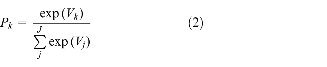
Time is an important dimension of travel choices; it is therefore essential to model time choice in transportation system analysis when evaluating travel demand management policies. The generalized extreme value (GEV) models ( 1 ), based on random utility maximization (RUM) theory, are the most important class of discrete choice models in travel behavior analysis, of which the multinomial logit (MNL) model is most widely applied ( 2 ). These models, despite their dominance in travel behavior analysis, are only used for discrete choice analysis. Some travel-related decisions are inherently continuous in nature; for example, time choices are typically continuous decisions, for which GEV models can only be applied when these variables are artificially discretized.
Using the GEV class of models for time-of-day (TOD) choice can take advantage of random utility theory. However, artificially dividing the time intervals results in adjacent time points being in different intervals; then the model considers them to be completely different alternatives but travelers may consider these time points as very similar.
The time interval boundaries are usually set in an arbitrary manner, as discussed by Bhat and Steed ( 3 ), without a reliable rule, and different model results can appear if the boundaries change. Considering correlations in discrete models can alleviate this problem to some extent, but a continuous treatment of time can solve the problem completely.
The continuous logit (CL) model, as a continuous extension of the MNL model ( 4 , 5 ), is able to take advantage of random utility theory when time is treated as a continuous variable, but requires non-time-varying variables (e.g., age, gender) to be time-varyingly handled. The currently used time-varying treatment of the utility function involves taking the form of an interaction with a trigonometric function of time ( 6 – 8 ), which causes the parameters of the utility function not to intuitively reflect the variable effect on time choice. An obstacle to model estimation is that the CL model requires numerical integration of the time-varying utility function for each observation, which greatly increases the computational effort and takes a long time to compute, thereby making it more difficult for applications with larger sample size.
In this paper, a finite mixture of continuous distributions is introduced to avoid the integration calculation of the model, which is still based on the framework of the CL model and therefore called the finite-mixture CL (FMCL) model. The proposed model not only retains the advantages of random utility theory, but also avoids the calculation of numerical integration, and more intuitively shows the influence of variables on time choice. Then simulation experiments of the FMCL model are conducted to verify the model estimation procedure. In an empirical study, the proposed model is applied for non-commuters’ shopping activity start time, based on Shanghai Household Travel Survey data, using the expectation-maximization (EM) algorithm. Non-commuting activities are chosen because the schedule of non-commuting activities is relatively flexible and has a larger choice space for demonstration purpose.
The remainder of the paper is organized as follows. The next section is a literature review of the TOD modeling, and is followed by a section that gives the equations of the CL model, the FMCL model, and the estimation method. The fourth section shows the simulation experiments of the FMCL model. The fifth section gives the results of the empirical study based on the FMCL model and the analysis of model estimation results. In the last section, some conclusions are drawn and some suggestions for future work are discussed.
Literature Review
TOD choice and time use are two important components of activity scheduling. Time use focuses on time allocation decisions, and capturing the interactions between duration, travel time, and activity–travel frequency. The fractional logit model, multiple discrete-continuous extreme value (MDCEV) model, and episode-based MDCEV model are mainly applied to the studies of time-use problems ( 9 – 13 ). Currently, the improvements proposed by Saxena et al. ( 12 ) and Palma et al. ( 13 ) for the episode-based MDCEV model are new advances in this field.
In the four-step travel-based demand forecasting model, the trip departure time is usually classified into a few peak and off-peak periods, for aggregating trip frequencies in each time period. As the focus of transportation planning shifts from long-term transportation infrastructure construction to short-term travel demand management policies, the activity-based travel demand model is more suitable for travel demand forecasting, which increasingly requires higher resolution of time measures, but time-choice modeling is still one of the main weaknesses of current activity-based travel demand forecasting models.
The TOD models in the literature can be divided into two main categories: (1) models that consider time as a discrete variable; and (2) models that consider time as a continuous variable.
The first category of time-choice models are discrete choice models, which can directly compute the choice utility of travelers and provide a convenient form for TOD choice models. However, these models require the division of time into discrete time intervals ( 14 , 15 ), and the interval boundaries are often arbitrarily set; nevertheless, the convenient structural form of discrete choice models has many advantages for model estimation and application. Discrete choice models have been used extensively in the literature for time-choice modeling.
Some researchers divided time into different time intervals and used MNL models to model commuting departure time choice ( 16 – 26 ). To address the property of the independence of irrelevant alternatives of MNL models, some researchers have applied the nested logit model ( 27 ), the cross-nested logit model ( 28 – 30 ), the ordered GEV model ( 31 – 33 ), the dogit ordered GEV model ( 34 ), the mixed logit model ( 35 – 38 ), or the multinomial probit (MNP) model ( 39 , 40 ) to solve the problem of correlations between alternatives. However, there is no robust theory to support the determination of interval criteria for time-choice discretization; Some researchers discretized time into 5–15-min intervals ( 16 , 17 , 24 ), some discretized time into 30-min to 1-h intervals ( 7 , 27, 41), and some divided time into morning and evening peak hours for study (14, 18, 20, 21, 30–33, 42, 43). The difference for interval division will place adjacent time points that are not much different for travelers into different time intervals, and this becomes a problem that cannot be solved using discrete choice models.
The second category of time-choice models treats time as a continuous variable and is further divided into two categories: (a) hazard duration models; and (b) continuous time-choice models based on RUM. The hazard duration models do not require discretization of time variables, but they are not based on RUM theory. Instead, they are based on a debatable assumption that the start time of the latter state only depends on the duration and end time of the previous state (3, 44–47). RUM-based continuous time-choice models include the CL model ( 48 , 49 ), the autoregressive continuous logit model ( 50 ), and the continuous cross-nested logit (CCNL) model ( 48 , 49 ). These models treat time as a continuous variable and have a good behavioral basis. The main difference between the CL model and the CCNL model is the latter’s ability to capture the correlation between alternatives that are similar in the continuous spectrum. Ghader et al. ( 50 ) proposed the autoregressive continuous logit model, which combines the CL model and the autoregressive process and can accommodate the correlation between alternatives in the continuous spectrum. Ghader et al. ( 51 ) introduced a Gaussian copula function based on a CCNL model to describe the correlation between the two dependent alternatives of activity start and end times.
The main advantage of both categories of continuous time models is that they avoid the arbitrary time interval settings that are required in discrete choice methods, and the problems that can be caused by time interval choice. The hazard duration continuous model is not a choice model based on RUM theory. For RUM-based models, the CL model requires one-dimensional integration calculations for each observation. The CCNL model and autoregressive CL model involve two- and multi-dimensional integration calculations, respectively, and the estimation time is longer than that of the CL model. Therefore, all the present RUM-based continuous models suffer from the problem of a time-consuming estimation process, which hinders the wide application of such models.
Methods
McFadden (
1
) proposed a class of multivariate extreme value distribution and then developed a GEV model for discrete choice applications based on this distribution and RUM theory. The model assumes that an individual will rationally choose the alternative with the highest utility value when making a decision. The utility

If the random error term
CL Model
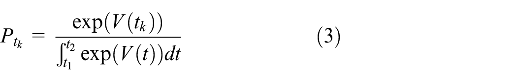
The CL model is a continuous extension of the MNL model. Suppose the lower and upper bounds of the continuous variable
The model can then be written in the form of the MNL model. As the interval
For identification purposes, all the explanatory variables need to interact with some continuous time functions. In addition, the function representing the TOD should have the same utility at

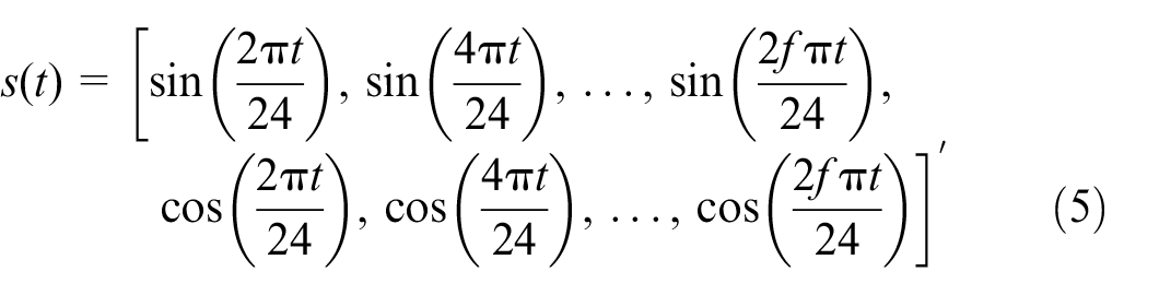
This utility function can equalize the utilities at
As shown in Equation 3, the CL model needs to calculate
Finite-Mixture CL Model
Utility Specification
The CL model can be used to obtain the probability density corresponding to each choice

Then the probability density is
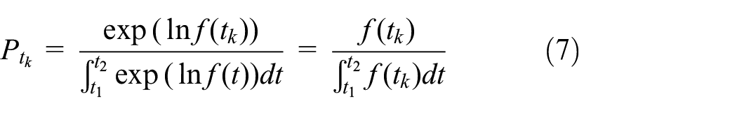
If

This utility specification would enable the choice probability density
Finite Mixture of Unimodal Distribution
Owing to heterogeneous preferences, people will have different choice preferences for time. People with the same choice preference may prefer to travel around a certain time point; the closer to that time point, the higher the density of the population distribution, thus forming a unimodal distribution. The time-choice distributions formed by people with different preferences often form a multimodal distribution.
The probability density distribution of activity start time choice of commuters is usually simple, with a unimodal or binominal distribution. However, the probability density distribution of the activity start time choice of non-commuters tends to be more complex, showing a multimodal distribution. Therefore, it is difficult to fit well using a single unimodal continuous distribution, which often does not reflect the actual distribution.
In this paper, the finite-mixture method is used to mix several unimodal continuous distributions together to jointly approximate a multimodal distribution of time choice. Let
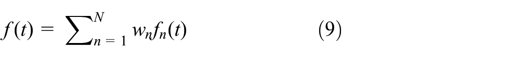
where
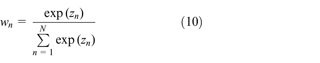
Here,

where
In addition, it is often assumed that the unimodal continuous distribution used for a finite mixture follows some common distribution (e.g., normal, Gumbel). It is necessary to evaluate and compare the goodness-of-fit of alternative density functions to choose a specific distribution. Based on the time-choice distribution characteristics of the actual data, the fit of the skew-normal and normal distributions were compared and the normal distribution was finally selected in this study.
When
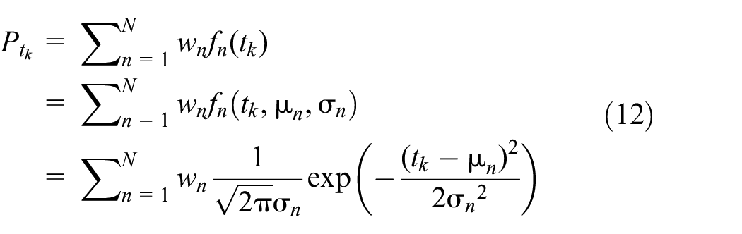
where
Next, we consider how the variables are incorporated into

where

where
EM Algorithms
The parameters
where
It has been noted earlier that maximization of the likelihood function using the usual Newton or quasi-Newton (secant) routines in such mixture models can be computationally unstable ( 52 , 53 ). To obtain good start values, Dempster et al. ( 54 ) developed a two-stage iterative method, which belongs to the EM family of algorithms.
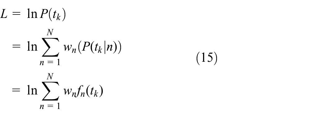
The EM algorithm consists of an E step and an M step, where the E step is to define an expectation and the M step is to maximize the expectation. For the EM algorithm, the log-likelihood function for an observation can be rewritten, as
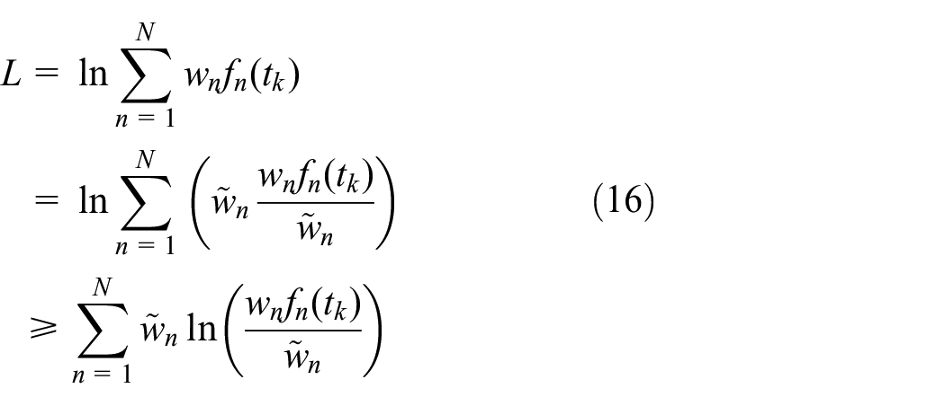
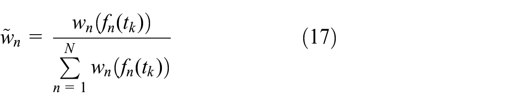
In the EM algorithm, the E step uses Equation 17 to calculate the weights of the normal distribution by guessing the initial values for the given parameters. In the M step, the weights calculated in the E step become constant values to maximize the likelihood function. Since the likelihood function of Equation 15 is fully concave for a fixed value of
Simulation Experiments
Before using survey data for empirical analysis, several simulation experiments are conducted to demonstrate the FMCL model and show whether the model estimation method is able to recover the parameters whose values are given in advance.
The simulation experiment is designed with a bimodal distribution obtained from a finite mixture of two normal distributions. A normal distribution is named Norm A, with
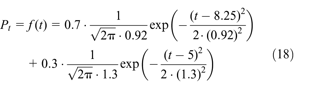
Table 1 shows the parameter estimation results of the FMCL model simulation experiments, and each parameter is significantly identifiable. The mean values of the parameter estimates are very close to the true values of the parameters. The standard deviation of the parameter estimates and the mean of the standard deviation estimates are basically the same, and the absolute percentage bias (APB) is less than 0.4% (
Simulation Results for FMCL Model (Repetition Number = 30)
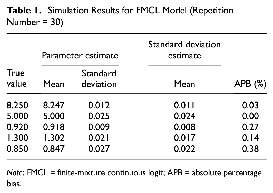
Note: FMCL = finite-mixture continuous logit; APB = absolute percentage bias.
Empirical Analysis
Data
The data were derived from the 2019 Shanghai Household Travel Survey, which surveyed 51,114 households and 111,511 individuals. The survey includes personal attributes, household attributes, and trip characteristics. Travelers are classified as commuters or non-commuters according to the purpose of the trip and whether the destination is the workplace or not. In this study, the activity start times of 10,048 home-shopping-home trips of non-commuters were extracted for analysis. The distribution characteristics of the activity start time are shown in Figure 1, showing a significant morning peak and a slight afternoon peak. This suggests that most non-commuters choose to shop at around 8:00 a.m., almost at the same period as the commuters’ morning peak, which further exacerbates the traffic congestion in the morning peak. Traffic congestion can be alleviated to some extent if trips derived from this relatively flexible schedule of shopping activities can be shifted to other time periods.
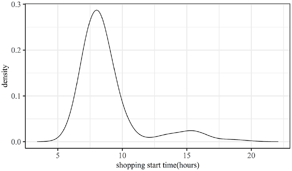
Distribution of travelers’ shopping start time choices.
Sample Description
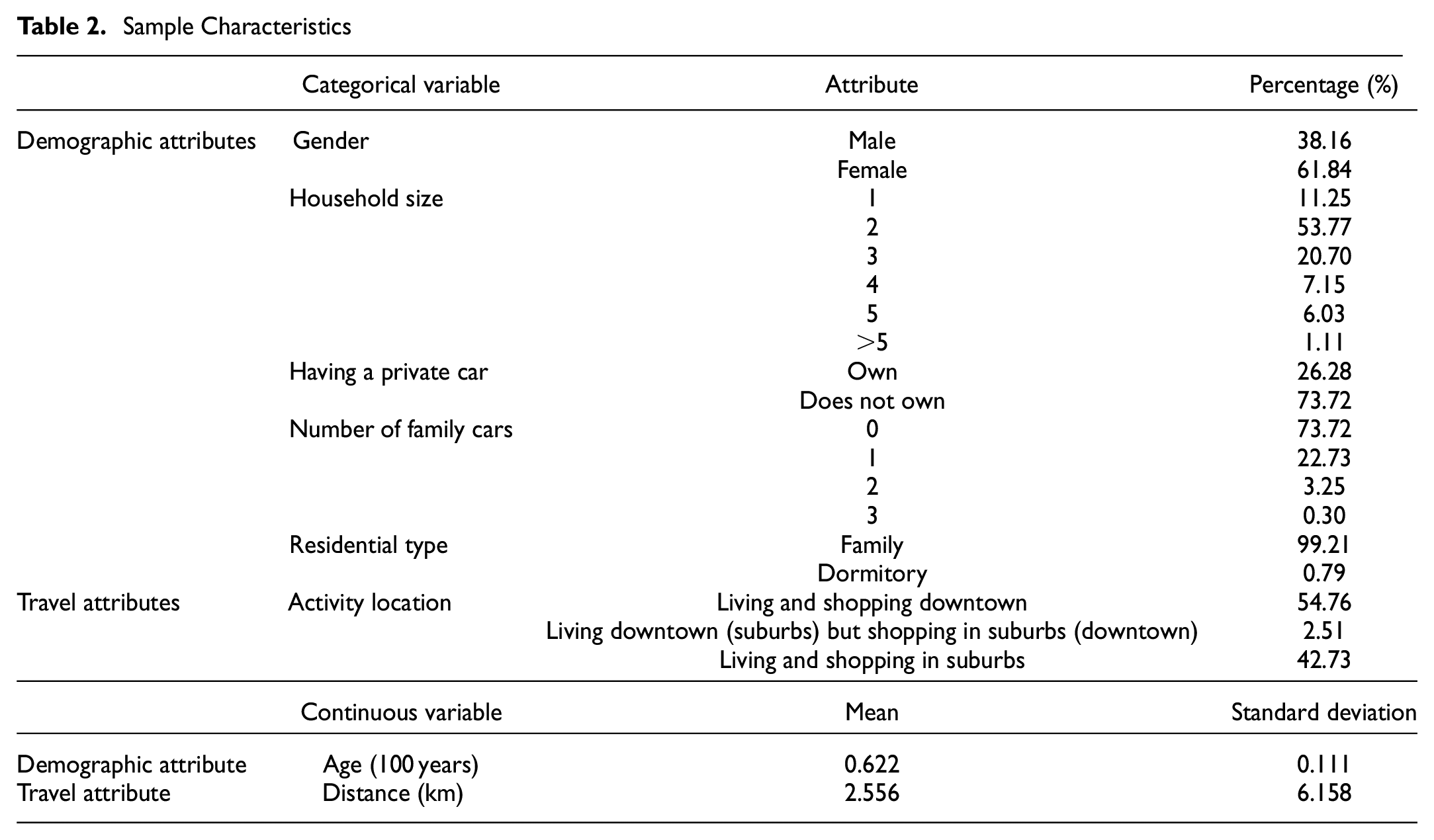
Table 2 gives descriptive statistics of the sample data, with 9754 travelers and 10,048 home-shopping-home trips. The table shows that the proportion of women in the sample data (61.84%) is higher than that of men (38.16%). The average age of non-commuters is over 60 years old. Most non-commuters have a household size of two people, do not own a car, and live with their families. The average trip distance of non-commuters is 2.5 km, and they are less likely to live in the suburbs and shop downtown, and vice versa. This indicates that, for shopping activities, people tend to shop close to their homes: those who live in the city center tend to shop in the central city area; those who live in the suburbs tend to shop in the suburbs; and fewer people live downtown and shop in the suburbs or live in the suburbs and shop downtown.
Sample Characteristics
Estimation Results
By comparing simulation results from two, three, and four latent segments, this paper uses four normal distributions to perform finite mixtures to fit the distribution of non-commuters’ shopping activity start times. The parameter estimation was performed in GAUSS software using the EM algorithm, and it took only 3 min to run with 10,048 observations on a computer with a CPU of 2.11 GHz and a RAM of 16 G.
Table 3 shows the FMCL model estimation results. The four normal distributions used for the finite mixture are named Norm 1, Norm 2, Norm 3, and Norm 4. The weight value in Table 3 is obtained by averaging the probability values of each individual entering the four normal distributions. The normal distribution with the highest weight is Norm 2 (81.82%), with
Model Estimation Results (N = 10,048)
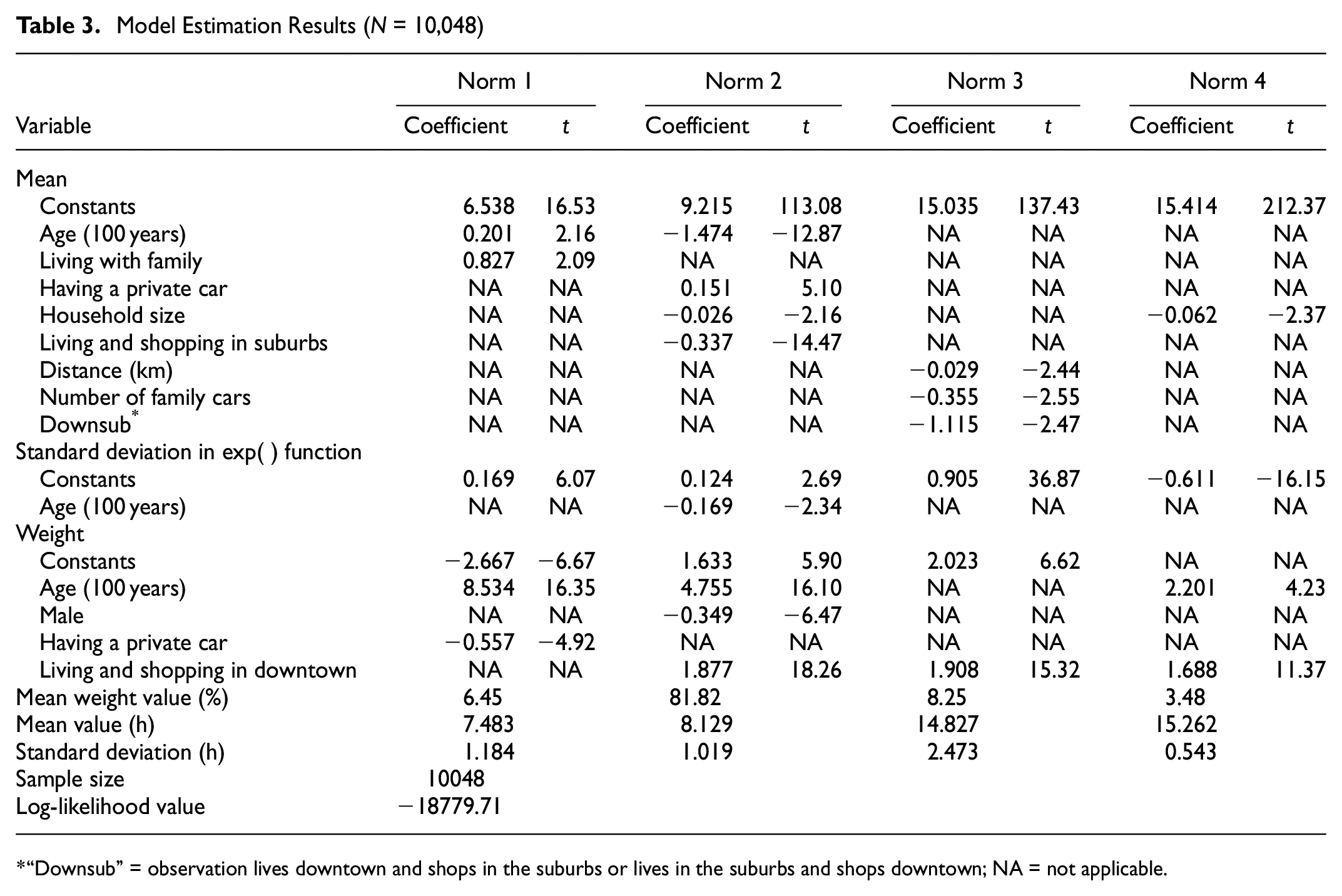
“Downsub” = observation lives downtown and shops in the suburbs or lives in the suburbs and shops downtown; NA = not applicable.
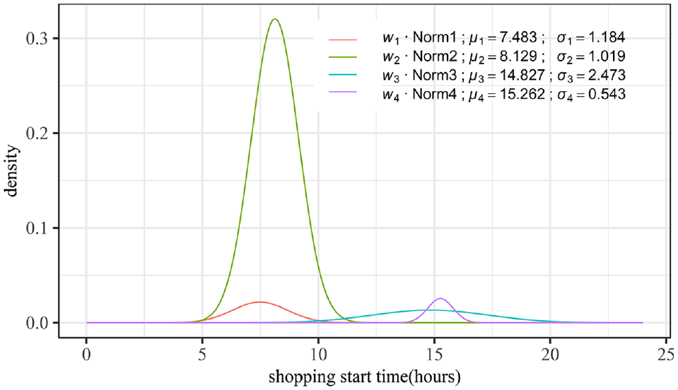
Four segments of normal distributions.
Norm 1 and Norm 2 together constitute the morning peak of the activity, and Norm 2 is the main part of the morning peak, while Norm 1 accounts for a small proportion and only plays a local adjustment role to the distribution. The two distributions are mixed together to better fit the real shopping activity start time of the morning peak. The actual meaning of the location parameter here is the average start time of the activity; that is, the average start time of the activity for people belonging to Norm 1 is 07:51 and the average start time of the activity for people belonging to Norm 2 is 08:07 The location parameters of the two distribution functions are very close. The sum of the weights of Norm 1 and Norm 2 is 88.27%, indicating that 88.27% of people choose to start their shopping activities at around 08:00 The average start time for Norm 3 and Norm 4 is 14:50 and 15:16 respectively, and the sum of weights for Norm 3 and Norm 4 is 11.73%, which means that 11.73% of people choose to start their shopping activities at around 15:00.
In Figure 3, we compare the actual shopping start time distribution with the finite mixture of the four normal distributions. Generating random numbers for each distribution as time points,
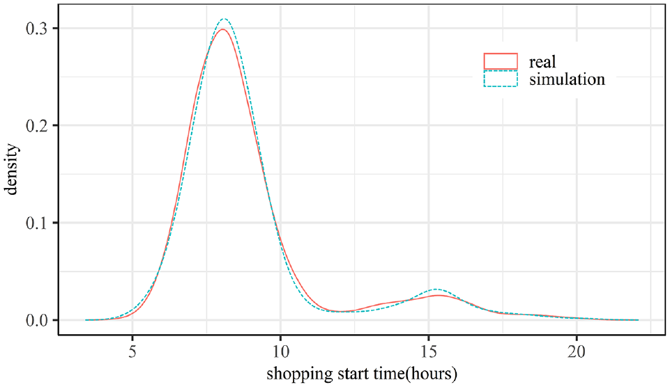
Comparison of model-fitted distribution and actual distribution.
For the morning peak, the fitted distributions are almost identical to the actual distributions, and for the afternoon peak, the fit shows a slight deviation. In general, the fitting effect is acceptable.
As shown in Table 3, the four variables “age”, “male”, “having a private car,” and “living and shopping downtown” significantly affect the probability that the traveler belongs to each latent segment of normal distribution. Older individuals tend to choose the distribution with an earlier activity start time; men are less likely to choose Norm 2. More women shop during this time period, probably because women undertake more shopping tasks in the household. “having a private car” has a negative effect on choosing Norm 1; this suggests that people with private cars at home do not tend to go out shopping early in the morning because it is very quick and convenient to go shopping by car. And “living and shopping downtown” has positive effects on choosing Norm 2, Norm 3, and Norm 4, which may reflect more characteristics of shopping activities downtown.
For Norm 1, the constant term is 6.538 (≈06:30) and the effect of both “age” and “living with family” on the mean value of Norm 1 is positive, indicating that people who are older and live with their families do not tend to start their shopping activities earlier than 6:30 a.m.
For Norm 2, the constant term is 9.215 (≈09:13). The effect of “age”, “living with family,” and “living and shopping in suburbs” on the mean of Norm 2 is negative, indicating that older people and people with larger households tend to start shopping activities earlier than 09:13 Possible reasons for this are that people from a large household need to undertake more shopping activities to satisfy the whole family, or that they also undertake more household chores and need to end their shopping activities earlier and go home. Older people tend to go shopping earlier in the morning, owing to their long-term habits (e.g., requiring less sleeping time and waking up early). The effect of “having a private car” is positive, indicating that households with cars tend to start shopping activities later than 09:13; a possible reason has already been described.
For Norm 3, the constant term is 15.035 (≈15:02) and the mean effect of “distance”, “number of family cars,” and “downsub” on Norm 3 is negative, indicating that the farther the distance between home and the shopping place, the greater the number of household cars and the greater the tendency of people start their shopping activities before 15:02. People living downtown and shopping in suburbs or living in suburbs and shopping downtown will have longer travel distances; this factor, together with the “distance” variable, suggests that people who travel longer distances tend to go out shopping earlier in the afternoon.
For Norm 4, the constant term is 15.414 (≈15:25) and the effect of “household size” on the mean for Norm 4 is negative, showing that people from larger households tend to start their shopping activities earlier than 15:25, possibly because more shopping tasks from household members push them to start shopping earlier.
The standard deviations of Norm 2 and Norm 4 are less than those of Norm 1 and Norm 3. One possible explanation is that people belonging to Norm 2 and Norm 4 are shopping in downtown areas, with a clearer purpose, and are more concentrated in the morning and afternoon peak hours. People belonging to Norm 1 and Norm 3 are shopping with an unclear purpose; thus the standard deviation is larger.
Conclusions and Discussions
Considering the application limitations of the CL model, this work combines the finite-mixture method and the CL model to develop a new continuous choice model, called the FMCL model. The model uses the finite-mixture method to mix several unimodal distributions together proportionally to construct a utility function. Embedding the novel utility function in the CL model allows the probability of individual choice to be obtained directly by calculating the probability density function of the continuous distribution. This improvement avoids the numerical integration calculation of the CL model, which simplifies the calculation of individual choice probability densities and reduces the estimation time of the model.
Reparameterization of the scale and location parameters for continuous distributions can quantify the effect of variables on continuous choice; this not only allows for an intuitive explanation of the effect of variables on the choice based on coefficients, but also retains a strong theoretical basis following the RUM principle to assess the economic welfare effect of alternative policies (e.g., Lemp and Kockelman [ 48 ]).
Several simulation experiments are conducted to demonstrate the FMCL model. Simulation experiment results show that each parameter is significantly identifiable and that the FMCL model can be estimated consistently. This paper also presents an empirical analysis of the FMCL model for activity start time choice in the context of home-shopping-home trips of non-commuters based on Shanghai Household Travel Survey data. The EM algorithm was coded in GAUSS software for parameter estimation, which takes only 3 min for 10,048 observations. A mixture of normal distributions was chosen to construct a utility function. A mixture function with normal distributions was constructed to fit the shopping activity start time distribution; the fitted distribution from the model is basically consistent with the actual distribution from the data.
The FMCL model has a well-defined probability density expression, and the simulation can be conducted by directly generating random numbers from those distributions. However, the CL model usually needs to be applied to the Metropolis–Hastings (MH) algorithm for simulation, which is relatively complicated and time-consuming. Therefore, the FMCL model also has the potential to reduce the simulation time.
It is worth noting that the proposed FMCL model can also be applied for welfare evaluation, which warrants the derivation of the model within the RUM framework. Ben-Akiva and Watanatada (4) showed that consumer surplus for the CL can be computed as the limiting formula for the MNL, as
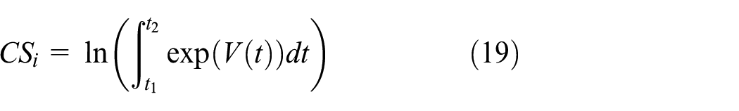
The welfare calculation formula is rewritten for the proposed FMCL model as
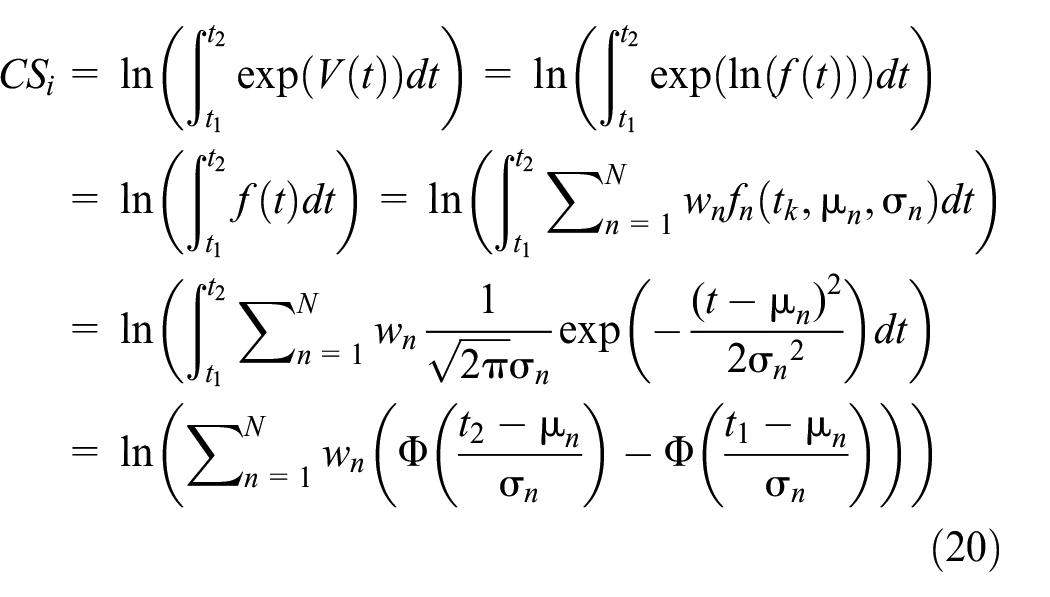
From Equation 20, the welfare in the FMCL model can be calculated based on the function of
For the utility function of the FMCL model, a finite mixture of other distribution functions can also be chosen for the construction, which has great flexibility for further extension and improvement. This study is just a first exploration on the finite-mixture model, which can be more widely applied to model continuous activity–travel decision variables in future.
Footnotes
Author Contributions
The authors confirm contribution to the paper as follows: study conception and design: X. Ye; data collection: T. Zhang; analysis and interpretation of results: S. Geng; draft manuscript preparation: S. Geng, X. Ye, T. Zhang, and K. Wang. All authors reviewed the results and approved the final version of the manuscript.
Declaration of Conflicting Interests
The author(s) declared no potential conflicts of interest with respect to the research, authorship, and/or publication of this article.
Funding
The author(s) disclosed receipt of the following financial support for the research, authorship, and/or publication of this article: Key project “Research on the Theories for Modernization of Urban Transport Governance” (No. 71734004) from the National Natural Science Foundation of China and project “Activity-Based Travel Demand Model Development for Shanghai” (No. kh0160020220382) from Shanghai Urban Planning and Design Research Institute.