
Abstract
Travel demand models regenerate the travel behavior of persons or households from scratch at every model run. However, the literature suggests that travel behavior remains relatively stable over time. Change in travel behavior is triggered by life events such as change in employment, household relocation, or birth of a child. The inability of existing travel demand models to represent habitual travel behavior and change in travel behavior of a person/household becuase of life events tends to exaggerate policy sensitivity and result in longer model run times to recreate travel behavior for every agent. In this study, we examined the travel behavior of persons between two consecutive years using a mobility panel survey from Germany. The travel behavior of persons with and without a life event is compared econometrically. Here, the travel behavior is measured as the number of weekly trips by activity type and mode and the impacts of six types of life events are studied. The results show that life events affect travel behavior, but the degree of impact varies by the type of life event, the trip purpose, and the mode. In some cases the impact is found to be negligible, but for many other cases the impact is profound. Moreover, general trends (not affected by life event) in travel behavior are also found. It is concluded that such dynamics in travel behavior should be represented by travel demand models for more sensible policy testing and computationally efficient travel demand models.
Traditional travel demand models recreate travel behavior from scratch every time the model runs. If a transport policy is tested at time
Travel behavior may differ a lot from day to day ( 1 ), but it does not change dramatically from year to year ( 2 , 3 ) because of the habitual nature of travel. Consumers are less likely to change their habits in stable environments, and interventions to change their habits are more likely to influence in cases where consumers environments are also changing (e.g., household relocation) ( 4 , 5 ). Verplanken et al. found that highly environmentally concerned university employees who moved residence used cars less frequently, or more frequently used environmentally friendly travel modes, to commute to university than employees who did not move residence or had low environmental concern ( 5 ). Life events, such as household relocation, graduation from school, change of job, birth of a child, and so forth, may change travel behavior fundamentally. But for most agents, such changes are rare. Even more, a policy scenario testing, for example, a toll road, does not have any influence on such life events. Conceptually, it is much simpler to recreate travel demand from scratch every time the transport models run. But it ignores habitual behavior, and thereby, exaggerates policy sensitivity.
Context
The long-term vision of this research is to build a transport model that covers travel of an entire week and adjusts travel behavior incrementally. The travel behavior of each agent shall be copied from the previous year and updated if:
By updating the travel behavior only after significant changes occurred to the household, the built environment or the network, changes in travel behavior, and thus, changes in levels of congestion, will be gradual ( 6 ). It is expected that simulating an incremental change to observed travel behavior is more realistic and significantly reduces runtimes compared with recreating travel behavior from scratch every time the model runs. It is further expected that logit models used to model the incremental adjustment of travel behavior require smaller constants than traditional models, and thereby, improve scenario sensitivity.
Similarly, the traffic assignment may be conducted incrementally. This idea was described by Wegener ( 7 ), where individual vehicles are added and removed from the network, while most vehicles remain unchanged. The assignment differs from behavioral choice models as agents typically select the shortest path based on an impedance function. Given that the path choice of one agent affects the travel times of many other agents, assignments typically run iteratively, resulting in longer runtimes. Unpublished work with MATSim conducted at the Technical University of Berlin has shown that an incremental assignment is possible if agents are maintained from year to year. It is expected that adjusting the assignment incrementally will substantially speed up this model step, as only those who are new agents or those who have changed their travel behavior need to find new paths in the assignment step. A user equilibrium should be found within a very few iterations, and thereby save model run time substantially.
As a first step, we analyzed the impact of life events on travel behavior changes, which is presented in this paper. This analysis is a first step for a transport model that updates travel behavior incrementally.
Literature Review
Socio-demographic attributes may explain in part the level of travel behavior variability ( 8 ). For example, unemployed people were found to have higher variability in their travel behavior. Typically, travel behavior is analyzed with cross-sectional survey data. Jones and Clarke provided evidence that multi-day data are needed to understand mechanisms behind travel behavior ( 9 ). Buliung et al. found that weekday-to-weekday travel behavior is more stable than weekday-to-weekend travel behavior ( 10 ). Therefore, a week-long travel behavior evaluation eliminates the fluctuations typical for given days of the week. Although a seven-day analysis does not represent all variations of an individual’s travel behavior, it does capture a reasonable sampling typical daily travel patterns ( 11 ). Tarigan and Kitamura analyzed a six-week survey and found that particularly the number of leisure trips over a week affect the variability of an individual’s travel behavior ( 12 ). The relative stability of week-long transit travel behavior was confirmed by Cui et al. ( 13 ).
The seminal study by Zahavi compared survey data from multiple metropolitan areas in the U.S. and concluded that travel time and travel expenses are relatively inelastic across different study areas ( 14 ). Although this finding strictly speaking does not confirm the hypothesis that individuals’ travel behavior is constant, Zahavi’s work provides evidence that travel behavior is relatively stable. It should be mentioned that some studies question the validity of Zahavi’s constant budgets ( 15 – 17 ). Mokhtarian and Chen explain, however, that travel time budget studies vary widely in relation to resolution (aggregate or disaggregate), modes included, unit of analysis (traveler, person or household), and statistical approach (Poisson regression, system of equations or survival analysis), which may affect the level of stability found ( 18 ).
Murakami and Watterson analyzed travel behavior of households in the United States using the Puget Sound Transportation Panel (PSTP) survey ( 19 ). The first and second waves of the survey were conducted in 1989 and 1990, respectively. Contrary to some of the studies described above, which found that travel behavior remains relatively stable, Murakami and Watterson found a slight reduction of household person trips between the two years ( 19 ). A larger increase in the average number of home-based work and non-home-based trips was found for people who changed their work location than people who remained at their workplace. For households who changed their residential location, a larger increase in home-based work trips and decrease in home-based other trips was found as compared with households who did not relocate.
For simpler transport analyses, traditional aggregate trip-based transport models are often sufficient ( 20 ). Many advanced analyses, however, require an agent-based representation of travel ( 21 ). Examples include modeling autonomous vehicles (AVs), ride-hailing, ride-pooling, demand responsive transport (DRT), urban air mobility (UAM), electric mobility, user-specific pricing systems, policies for peak-spreading, equity analyses, and others.
In response, activity-based models were designed to represent travel behavior at the agent level. In such models, the travel itself is not modeled as a motivation, but rather the desire to carry out activities at different locations ( 22 – 24 ). Several activity-based models were built in response (such as ActivitySim, ADAPTS, ALBATROSS, CEMDAP, CT-RAMP, FEATHERS, actiTopp, MOBi.plans, SimMobility or TASHA) that have greatly improved the ability to analyze scenarios ( 25 ). actiTopp even models weekly travel plans ( 26 ). Nevertheless, only a minority of transport modelers uses activity-based models today. The vast majority continues to use aggregate trip-based models, ignoring many of their limitations ( 27 ).
As powerful as activity-based models are, they typically carry three substantial limitations. Most activity-based models work with many and comparatively large constants. Discrete choice models ( 28 , 29 ) are the backbone of activity-based models. Such models are estimated and calibrated to reflect observed tour generation, destination choice, tour mode choice and trip mode choice, intermediate stops, and time-of-day ( 30 ). Although these models represent observed travel behavior very well, they often depend on relatively large constants in activity-based models. Many and large constants help to match observed data, but they limit the model’s policy sensitivity. Second, most activity-based models suffer from substantially longer runtimes ( 20 ). And finally, just as their trip-based counterparts, activity-based models forget travel decisions of previous years and recreate travel behavior from scratch in every simulation period. Thereby, habitual travel behavior ( 31 ) and attitudes ( 32 , 33 ) are ignored.
Method
To explore econometrically the stability of travel behavior over time, panel data were analyzed. The German mobility panel (MOP) dataset provides week-long travel behavior data since 1994 on a yearly basis. The same 500 households are asked to fill in a travel diary survey three years in a row. The travel diary covers an entire week with seven days. Data for the most recent nine years, from 2010 to 2018, were chosen to reduce the long-term change in travel behavior resulting from increasing income and declining household sizes. The sample size over the last nine years is 6,922 households with 11,562 persons. However, after cleaning the data for missing records and inconsistencies, the final dataset used for analysis contains 4,043 households with 6,508 persons.
Travel behavior is likely to change from day to day, but the literature review suggested that the week-long average is comparatively stable ( 3 ). This dataset covers an entire week of travel, which helps to identify changes that are triggered by life events rather than random differences from one day to the next. This longitudinal dataset allows us to describe the stability in travel behavior over time as well as the disruptive effect of life events on travel behavior. This paper focuses on the analysis of week-long stability of travel behavior from year to year. Average change, standard deviation and outliers are analyzed econometrically.
Travel Behavior
In this study, we consider travel behavior as the number of trips by activity type and mode. The activity types considered are work, education, shopping or errands, leisure or hobby, pickup or drop-off, recreational round trips, and other. Four travel modes are distinguished, including walk, bicycle, car, and public transport. The travel mode car includes car as a driver, car as a passenger, moped, and motor bikes. The travel mode public transport includes city bus, long-distance bus, light rail, subway, and regional and long-distance trains. The change in travel behavior is considered as the difference in total weekly trips between two consecutive years.
Life Events
Many life events potentially affect the travel behavior of households and persons. In this study, we considered six life events that we were able to detect in the panel data. These events are change in employment status of a person, change in household size, change in household income, birth of a new child, change in household car ownership, and household relocation.
The MOP dataset collects employment information of a person including categories such as full-time, part-time, homemaker, and retired. We categorize employment as Employed and Unemployed. The employed category contains full-time and part-time workers, and the rest of the categories are grouped as unemployed. The travel behavior of persons with change in employment status from employed to unemployed or unemployed to employed is compared with persons who remain employed or unemployed over two consecutive years.
The variable household size is collected as the total number of people living in a household. The travel behavior of households whose size increases or decreases between the two consecutive years is compared with households with a constant household size. Unfortunately, the dataset does not allow us to identify unambiguously if a household lost one person and added another person in the same year. This occurrence is assumed to be rare and part of the category constant household size. The birth of a child can be identified without doubt and is compared with households that did not have a newborn added to the family.
The change of car ownership refers to the change of number of cars permanently available to a household and is represented by four categories. These categories are car ownership increased, decreased, remained the same, and remained car-free between two consecutive years. The data do not allow us to detect if a household replaced a car, but this change presumably has limited impact on the number of trips. Replacing a car is therefore captured in the category car ownership remained the same. Finally, the household relocation status describes whether a household relocated or remained at their location between the two consecutive years.
Whereas life events are household events, the travel behavior is analyzed at the person level. Although most transport models in North America work at the household level, most models in the UK work at the person level. Pokhrel found no substantial difference in model fit between person and household level ( 34 ). The person level was chosen here to detect shift of trip-making between household members. A household may experience a single life event, multiple life events, or no recorded life event between two consecutive years. Table 1 shows persons by number of life events experienced by their household. About 18% people experience a single life event and around 6% people experience more than one life event, as shown in Table 1.
Summary of Life Events Between Two Consecutive Years
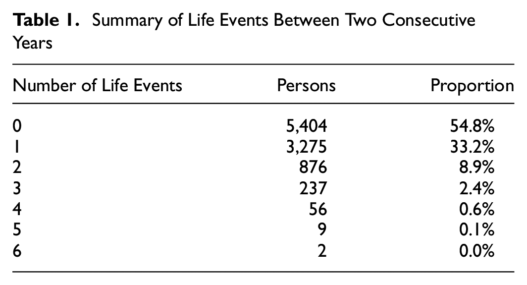
In this study, we compared the travel behavior of people with no life event with people with a single life event. Multiple life events were excluded from the analysis, as it would be impossible to detect which specific life event triggered travel behavior change to which degree. The number of observations with multiple life events is too small to explore econometrically, at least when specific life event combinations (such as birth of child + relocation) are explored. Therefore, as a first step, we only consider mutually exclusive life events.
Results
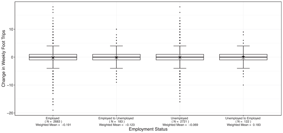
The change in travel behavior is considered as the difference in total weekly trips between two consecutive years. The change in weekly trips by activity and mode in response to the life event change of employment is presented in a series of boxplots. Figure 1 shows change in weekly work trips by four categories of employment status. The cross symbol in each boxplot shows the sample mean, whereas the dot symbol shows the weighted mean using expansion factors from the survey data. The x-axis of Figure 1 also shows the sample size in each category of employment, including the weighted mean value. In this study, we consider six life events and eleven types of travel behavior change, which results in sixty-six figures representing change in trips by activity, mode, and life event. In this paper, we only present selected results for employment status in boxplots, and all other analyses are shown with weighted averages in Tables 2 and 3.
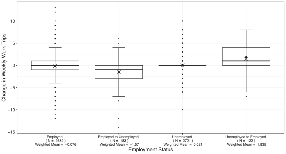
Change in weekly work trips by employment status.
Weighted Average Change in Weekly Number of Trips by Purpose and Life Event
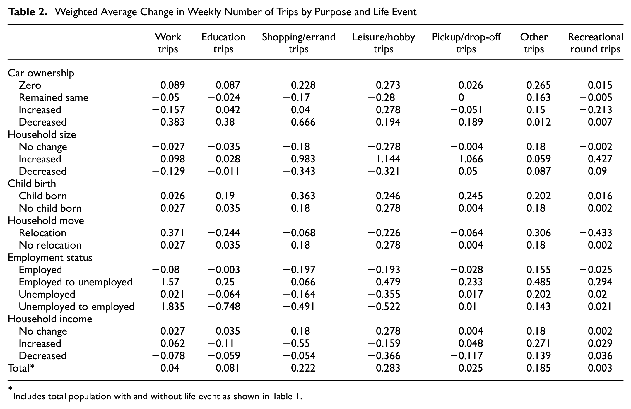
Includes total population with and without life event as shown in Table 1.
Weighted Average Change in Weekly Number of Trips by Mode and Life Event
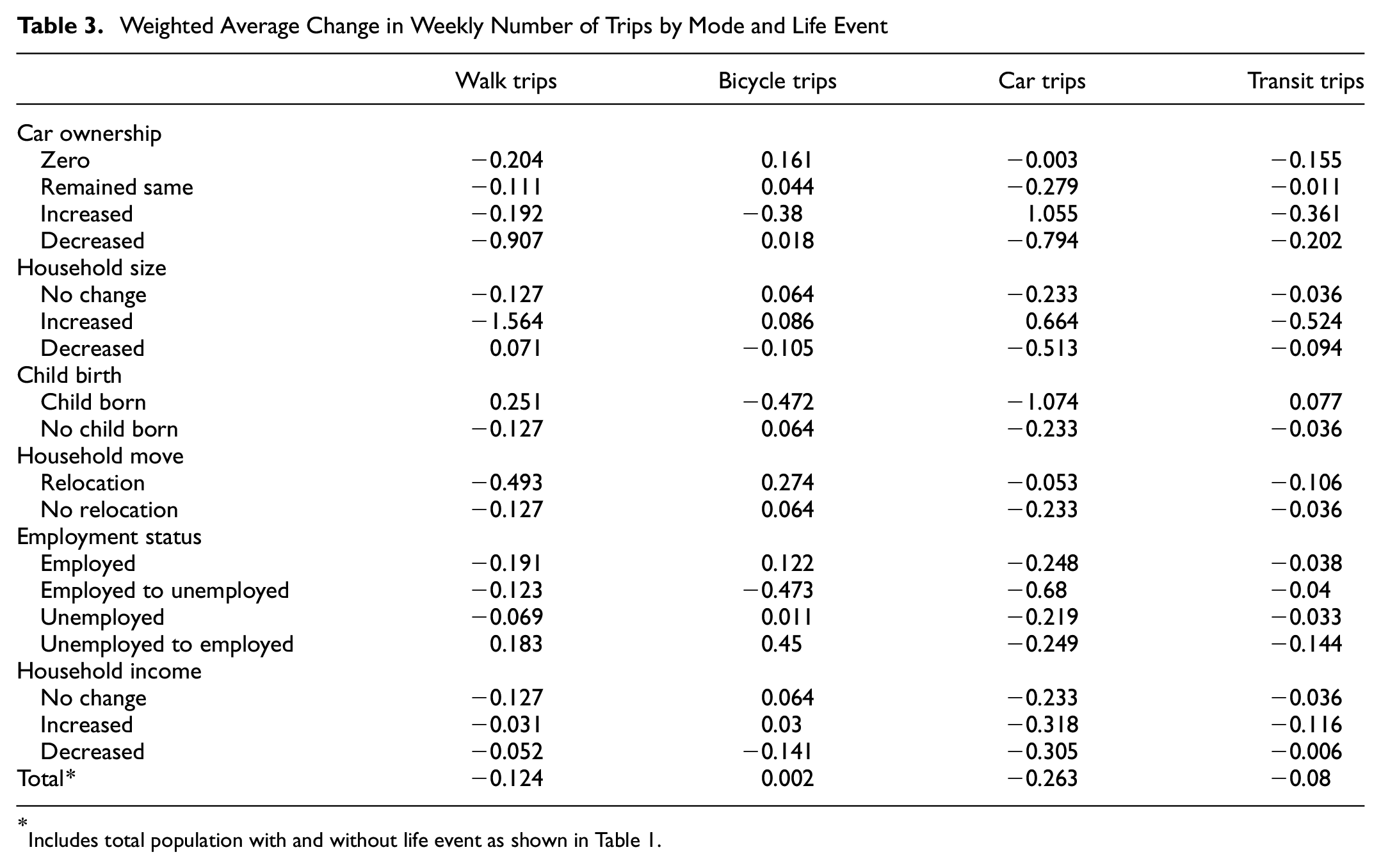
Includes total population with and without life event as shown in Table 1.
Life Event: Employment Status
Figure 1 shows that the change of weekly work trips is greater for people who changed their job status (i.e., started a job or became unemployed) than for people who stayed either employed or unemployed. For people who got employed from an unemployed status, the weekly work trips increased with a population-weighted average of 1.7 trips. The boxplot (fourth boxplot in Figure 1) is above zero, showing that 75% of all these persons increased their number of weekly work trips after starting a job. There are a few people, however, who conducted fewer work trips than the year before. These are cases where people might have done many job interview trips and trips to the unemployment office (which are counted as work trips) while being unemployed. The week they reported their trips after starting a job might have been a week where they were on sick leave or taken paid time off.
Similarly, people who became unemployed reduced the weekly work trips with a population-weighted average of −1.8 trips, shown in the second boxplot in Figure 1. Again, 75% of those reduced the number of work trips, but a few have conducted more work trips possibly to attend job interviews. The weekly work trips remained relatively stable where people remained either employed or unemployed. The variation for people who remained employed is larger than for people who remained unemployed, as employed people typically do many more work trips than unemployed people, providing more room to change the number of weekly work trips. As expected, the largest variation in weekly work trips is found for people who changed employment status between two consecutive years. The outliers in Figure 1 might be the result of non-typical weeks when the respondents were surveyed.
Figure 2 shows a very small increase in education-related trips when a person becomes unemployed, probably as a result of starting training or going back to school. For the other employment status cases, the number of education trips remained rather stable. This is not surprising, as most people who are employed or unemployed (but not students) do not conduct education-related trips. Weekly trips for shopping or errands (Figure 3) are also affected by a change in employment status. The weekly shopping or errands trips decreased for persons who started a job and increased for those who became unemployed. There is also a small reduction of shopping/errands trips for persons who remained employed or unemployed, which possibly represents an increasing trend toward online shopping ( 35 ). Similar trends are observed for leisure or hobby trips, as shown in Figure 4. However, about half of the respondents reported a reduction in leisure/hobby trips after the employment status changed from employed to unemployed. This might be related to the reduction of disposable income, which might limit leisure activities of some people who became unemployed. Their variation of change in weekly trips is higher than for other categories of employment status, indicating a heterogeneous impact of becoming unemployed on leisure trips (Figure 4).
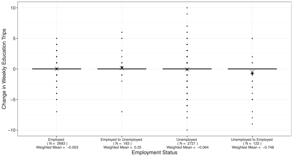
Change in weekly education trips by employment status.
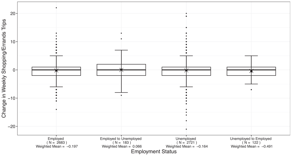
Change in weekly trips for shopping or errands by employment status.
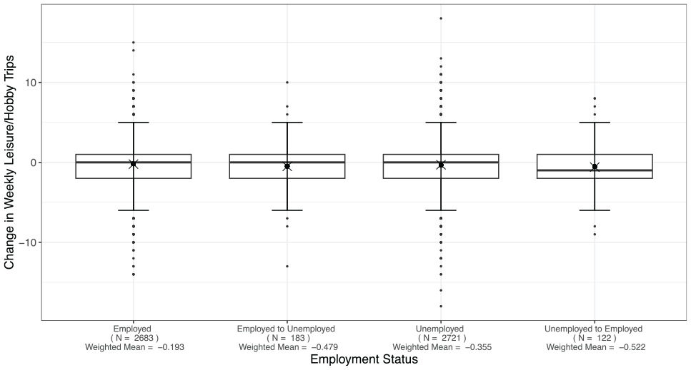
Change in weekly leisure/hobby trips by employment status.
Figure 5 shows change in weekly pickup or drop-off trips by employment status. Those who became unemployed tended to do more pickup and drop-off trips as compared with those who started employment. Those who remained employed marginally decreased the number of pickup/drop-off trips, whereas those who remained unemployed by and large did not change travel in this category, with the exception of some outliers (Figure 5). Recreational round trips, such as going for a run or taking the dog for a walk, are remarkably stable for all employment status categories, as shown in Figure 6. Other types of trips, such as visit a doctor, visiting a friend, or going to a bank (Figure 7) were relatively stable with a small trend to increase the number of trips for all employment status categories. The variation in weekly other trips is slightly higher for those whose employment status changed from employed to unemployed (Figure 7).
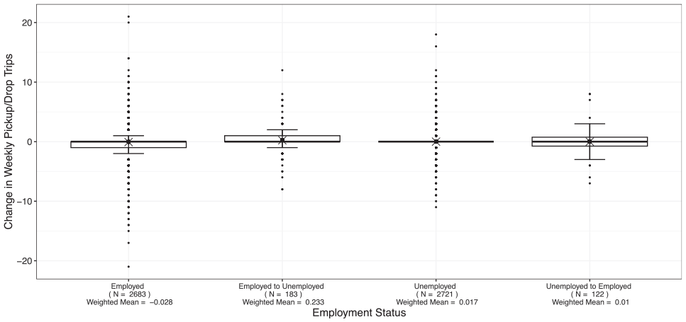
Change in weekly pickup/drop-off trips by employment status.
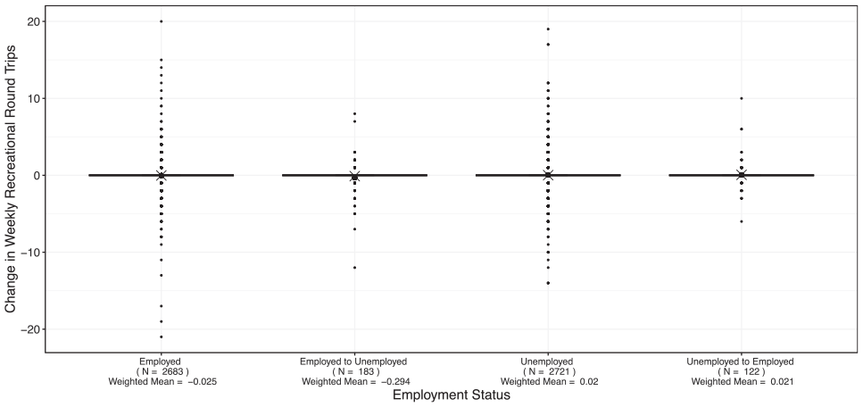
Change in weekly recreational round trips by employment status.
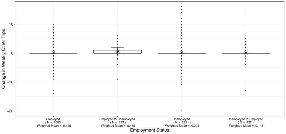
Change in weekly other trips by employment status.
Next we looked at the impact on mode choice, represented as number of trips by mode and change in employment status. Figures 8 and 9 shows the impact of employment status change on change in weekly car and public transport trips. Figure 8 shows that the change in weekly car trips remains relatively stable, even though there is quite some spread in change of car trips. Car trips are made to fulfill many activities, including work. Although people may conduct more or fewer car trips from one year to the next, change of employment status appears to be a poor predictor for number of car trips. Similar results are found for public transport trips (Figure 9), which remained rather stable in response to change in employment status with even less variation than for car trips.
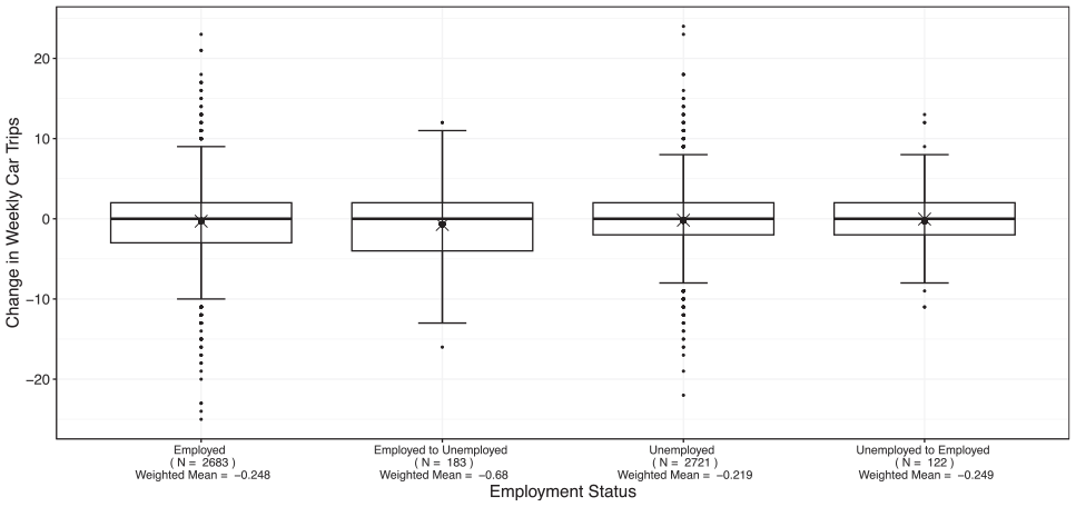
Change in weekly car trips by employment status.
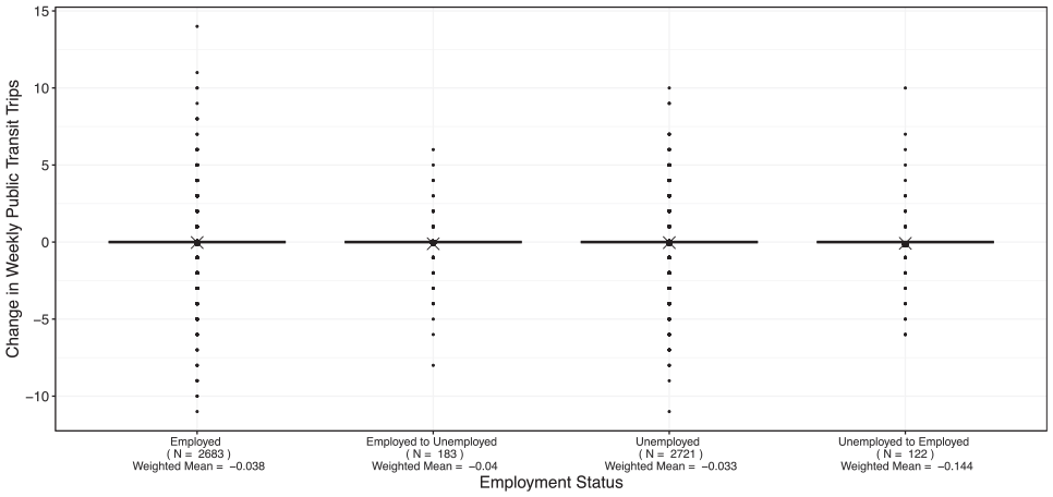
Change in weekly public transport trips by employment status.
The change in weekly trips by active transport modes is shown in Figure 10 for walking and Figure 11 for cycling. Those who started employment increased the number of weekly walk trips than other categories of employment status (Figure 10). Work trips tend to be the longest trips, making walking less likely and reducing the time window for other walk trips. The variation in weekly bicycle trips is very small. Figure 11 shows a small increase in weekly bicycle trips when a person becomes employed and decrease when a person becomes unemployed. In Germany, 11% of all trips are done by bike, and 18% of commute trips are cycled ( 36 ).
Change in weekly walk trips by employment status.
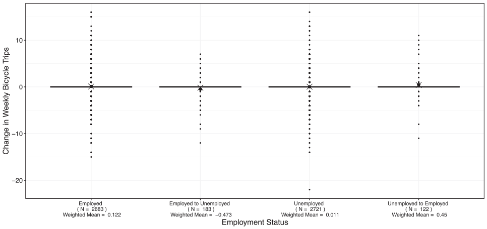
Change in weekly bicycle trips by employment status.
Life Event: Car Ownership Status
The car ownership status distinguishes whether a household does not own a car, the number of cars remained the same, increased or decreased between two consecutive years. Table 2 shows a decrease in weekly work trips with a decrease in number of cars owned by a household. This is likely caused by some workers not driving home in the lunch break and other workers opting for working from home after reducing the number of cars. The causal relationship might also be that some people sold a car after working from home became possible. For other categories in car ownership the change in work trips was marginal. Work trips are trips and car ownership is likely to influence the mode of commute trips but less the number of work trips. The impact of the car ownership status is very similar to commute trips for education trips, trips for shopping and errands, leisure trips, and trips to pick up or drop off others. Recreational round trips and other trips are barely affected by the car ownership status.
Table 3 shows the impact on trips by mode of transport subject to a change in car ownership status. As expected, weekly car trips tend to increase with an increase in car ownership, whereas trips by other modes clearly decrease on the average. With the decrease in car ownership, weekly car trips tend to decrease whereas bicycle trips tend to increase. We would like to highlight here that car ownership is a household variable and the trips are person trips. Therefore, it is important to note that a car might not be available to all members of the household, and some household members might not even have a driver’s license.
Life Event: Household Size
The change of household size is caused by several reasons, including a child leaving the parental household, a household member passes away, or the birth of a new child. Unfortunately, the panel data did not allow us to determine the reason for the change in household size. Although birth of child could be analyzed as a separate event, the other events that cause a change in household size could not be intensified unambiguously. Therefore, all events that affect the household size were taken as a single life event change of household size.
Table 2 shows that the impact of a household size change on work and education trips is minor. Weekly shopping and errand trips were reduced by a similar margin as shown in the employment status in Figure 3, and likely reflect the general trend in reduction of shopping/errands trips in this longitudinal dataset. Weekly leisure or hobby trips increased if the household size dropped in two consecutive years. This might reflect additional free time after a child moved out or a relative passed away that might have needed care. Weekly pick up or drop-off tended to increase the most with increase in household size, most likely caused by the need for daycare after giving birth to a child. Other types of trips tend to be relatively stable and were not notably affected by a change in household size.
Table 3 shows that weekly walk trips tended to decrease with an increase in household size and vice versa, whereas car trips show the opposite pattern. This might reflect the additional coordination needed in larger households, which sometimes might be easier to accomplish by a car. Many walk trips might be leisure or hobby trips which show a similar trend (Table 2). Bicycle trips tend to increase with a growth in household size and decrease with a reduction in household size.
Life Event: Child Birth
The impact of the birth of a child on travel behavior was expected to be substantial, and was therefore analyzed as a separate set in addition to change of household size. Overall, Tables 2 and 3 show a decrease in most of the weekly trips by trip purpose and travel mode. For example, there is a reduction in weekly work and education trips possibly as a result of parental leave, which is paid up to 14 months in Germany. However, variation in weekly work trips (based on the boxplots not shown in this paper) is higher than weekly education trips, indicating that there is a wide range of reaction to the birth of a child. Weekly trips dropped by all modes except public transport, as shown in Table 3. There is also more variation in weekly trips by car than by public transport observed in the data.
Life Event: Household Relocation
Household relocation is based on the survey question whether the household relocated from one year to the next. Table 2 shows that weekly work trips tend to increase with household relocation. Moving closer to a workplace location often is a driver of household relocation ( 37 ), and the new housing location might be more convenient for more frequent trips to work. Education trips, on the other hand, dropped after relocation. This might have been caused by students who graduate and move to another place to start their first job. Leisure and hobby trips dropped whereas other trips increased, possibly related to many trips after a move to set up the new home. We further attempted to analyze the direction of a move (distinguishing moves between cities, suburbs, and rural areas). However, the number of households moving from one area type to another was very small at 7%. Unfortunately, there were some inconsistencies in the data where a different area type was coded for the same household in two years but the relocation attribute was set to false. The actual location of a household was not disclosed for privacy protection. We were not able to sort out this inconsistency, which might be caused in part to area types changing over time and in part to incorrect responses in the survey. To reduce this uncertainty, we did not explore the attribute area type further.
Weekly walking trips (Table 3) tended to drop with household relocation. There is a lot of variation in change of weekly car trips (probably because of the built environment of the new housing location), but on the average, the weekly car trips tended to drop just slightly after household relocation. Finally, weekly transit trips tended to reduce substantially after a household relocates compared with households who did not move. In part, this might reflect ongoing urban sprawl, which would also be supported by a reduction in walk trips (Table 3). However, the quality of the data did not allow for further analysis of area types before and after the move.
Tables 2 and 3 showed a small reduction of trips for the entire surveyed population. This is confirmed by the cross-sectional survey MiD (Mobilität in Deutschland) from 2008 and 2017, which showed a reduction of 6.5% in urban travel and also by the PSTP survey in the United States 19 ).
Conclusions
To the best of our knowledge, this paper presents the first comprehensive study of the impact of life events on change of travel behavior. Whereas travel behavioral may change substantially from day to day, it remains comparatively stable if aggregated to weeks or even months. Understanding incremental changes to travel behavior helps to explain sensitivities to new policies, and thereby, avoids overstating the impact of the policies.
Positive and negative impacts of life events on number of trips by purpose and mode calculated in this research were plausible and within expected ranges. The individual impact of life events, however, has a large range of effects on the individual travel behavior. For example, those who changed from unemployed to employed from one year to the next ranged from reducing the number of weekly work trips by seven to increasing the number of weekly work trips by nine (compare right boxplot in Figure 1). Obviously, more aspects affect the number of weekly work trips from one year to the next, including taking time off, sick leave (of the worker or of a dependable person in the same household), business travel, working from home, choice to go home for lunch, need for job interviews, and trips to the unemployment office, among others. For discretionary travel, even more variation is expected, influenced by the mood to travel, the perceived necessity to travel, the weather or the health status, just to mention a few. Not all of these can be measured in travel surveys, and therefore cannot be represented explicitly in transport models. Given the remaining unexplainable changes in travel behavior, some random effect in agent-based models will remain appropriate. However, the more elements we are able to move from random effect to explainable effects with empirical evidence, the more meaningful the policy sensitivities in transport models will become. Overall, a general trend of reduction in weekly trips throughout the population, that is, persons with or without a life event, is also observed, except for the activity type other trips and mode type bicycle trips. However, the degree of reduction in weekly trips varies among activity types (Table 2) and travel modes (Table 3).
A limitation of this research is the relatively small dataset with 10,139 records since 2010, of which only 1,781 persons experienced one of the studied life events. However, panel surveys are rare, particularly panel surveys that capture week-long travel behavior. Although it is easy to complain that a given dataset is smaller than desired, the German MOP data provide an unusual opportunity for longitudinal travel behavior analyses.
In this paper, we analyzed travel behavior with regard to number of trips. Another interesting travel behavior outcome is trip lengths. All analyses shown in this paper were also conducted with trip length. It turned out that the variation in trip lengths was smaller than in number of trips. In other words, life events were more likely to affect the number of trips than the traveled distance per week. One could have expected that it would have been easier to adjust the destination (such as selecting a grocery store that is closer) than adjusting the number of trips. Apparently, respondents tended to travel similar distances, even if they did fewer trips. This finding might confirm Zahavis’s ( 14 ) theory of constant travel time budget. It is possible, however, that this is an artifact of this survey. The survey does not contain coordinates of origins and destinations but self-reported trip distances. As respondents tend to round survey responses, it is perceivable that the rounded values tended to be similar, even after a life event occurred, whereas the number of trips might have been reported more truthfully. With the given data, however, we were not able to confirm this hypothesis.
As a next step, we plan to explore the impact of life events in conjunction with socio-demographic attributes. It is possible, for example, that the birth of a first child has more impact on travel behavior than the birth of a second child. Likewise, buying a car might have a larger impact for a young driver on travel behavior than for a retiree. Furthermore, we are interested in exploring not only trips by purpose and trips by mode separately, but also in exploring the cross-tabulation of the two dimensions. Impact on trip length is another intriguing analysis. Last but not least, we are interested in analyzing the complementary effects of multiple life events happening in one year. Will the decreasing effect of the birth of a child on work trips cancel out with the increasing effect of household relocation on work trips? Or will one life event dominate over the other? Certainly, the small sample size of 576 persons with multiple life events in one year will limit the ability to quantify the impact of simultaneous life events. But there might be typical combinations, such as birth of a child and household relocation, that were observed with sufficient frequency to be analyzed econometrically.
We also plan to explore the relationship between life events and change of travel behavior through the lens of explainable (xAI) and interpretable artificial intelligence (iAI). We intent to train various prediction models that range from random forests and gradient boosted trees toward (deep) neural networks to explain the impact of single and multiple life events and their interaction with socio-demographic attributes on travel behavior. Then, an interpretable representation of a decision tree of a random forest will be used for counterfactual analyses, which will help to explore what-if analyses of unseen cases ( 38 ).
Footnotes
Author Contributions
The authors confirm contribution to the paper as follows: study conception and design: R. Moeckel, U. Ahmed; analysis and interpretation of results: U. Ahmed, R. Moeckel; draft manuscript preparation: R. Moeckel, U. Ahmed. All authors reviewed the results and approved the final version of the manuscript.
Declaration of Conflicting Interests
The author(s) declared no potential conflicts of interest with respect to the research, authorship, and/or publication of this article.
Funding
The author(s) received no financial support for the research, authorship, and/or publication of this article.