
Abstract
Travel surveys generally rely on single-day travel diaries where respondents report their travel information for a typical weekday. However, the concept of a typical weekday does not represent the current reality, as travel behavior has been largely altered in the post-pandemic period. Besides, the conclusions based on analyzing single-day travel diaries lack the ability to capture daily variations in travel behavior. In response to these concerns, this research proposed a framework to expand single-day travel diaries into longitudinal multi-day travel data using a pseudo-panel approach. Leveraging the constructed longitudinal data, the study evaluated the determinants of people’s daily participation in work–school, routine, and discretionary activities. Fixed and random effects panel data estimation models were used for this purpose. Results showed that activity participation is largely attributed to vehicle ownership, income, education, driving license, and household structure. Noticeable daily trends were observed in work–school and discretionary activities. A negative association between transit pass ownership and activity participation was noticed, suggesting social exclusion faced by transit users. In addition, teleworkers were found to be relatively more engaged in discretionary activities. Suburban residents were found to travel longer to participate in activities compared to urban dwellers. The proposed research framework can support future activity-based modeling aspects, such as activity participation, scheduling, mode choice, shared travel, and destination choice models, specifically addressing the “typical weekday” barrier.
Keywords
The imposed travel restrictions during COVID-19 have caused a significant shift in people’s daily travel behavior. As we enter the post-pandemic era, the effects are still observable in people’s mode choice, shared travel, and activity participation decisions ( 1 , 2 ). New mobility opportunities, such as telecommuting, teleworking, hybrid/fully work-from-home, online shopping, and so forth, have significantly altered the work/non-work trip patterns in the post-pandemic period ( 3 ). Transportation planners and professionals largely rely on cross-sectional survey data to examine travel behavior and system performances where respondents are asked to report their travel information for a “typical day of the week.” However, as established from a large pool of post-pandemic travel behavior research ( 3 – 6 ), the idea of a “typical day” does not exist anymore given varying work arrangements. Besides, conclusions drawn from analyzing single-day travel diaries fail to measure the daily variation in activity participation. Multi-day travel information not only captures the time effect on travel behavior but also provides a better representation of socio-demographic, location, and travel resource-related determinants of activity participation, as impacts can be measured across time and space. Some researchers have utilized genuine longitudinal panel data to overcome this issue, where an individual’s travel information is collected for a week or more. The German Mobidrive survey is an example of such an initiative, where six weeks of travel logs were collected from 139 participating households to explore the impact of seasonality and long-term travel attributes ( 7 ). Good quality panel data, however, is difficult to acquire because of the high cost, small sample size, and lack of representativeness ( 8 , 9 ). Therefore, studies exploring the temporal effects on travel behavior are scarce.
An alternative to the genuine panel is the application of a pseudo-panel, created by stitching together repeated cross-sectional data from different timelines to mimic longitudinal data. The pseudo-panel concept was first proposed by Deaton ( 10 ). The difference between a genuine panel and a pseudo-panel is that similar individuals are not observed over time; rather, samples are drawn from waves of cross-sections from a pool of cohorts. This pool of cohorts can be addressed as groups where individuals with similar attributes are placed. The attributes are generally time invariant in nature and exhibit high within-group similarity and between-group dissimilarity. Different fields of study, including the transportation domain, have utilized this method to estimate time effects from repeated cross-sectional data. Weis and Axhausen ( 11 ) studied the induced travel demand and aggregate effects of altered generalized cost on an individual’s travel behavior based on Swiss National Travel Survey data collected at 5-year intervals since 1974. They followed the pseudo-panel approach to generate longitudinal time-series data from seven repeated cross-sectional surveys. They considered birth year, gender, and region as cohort sub-dividers to obtain 838 observations. To assess the impact on mobility, variables such as age, household size, employment, car ownership, number of trips, out-of-home trips, duration of out-of-home activities, and trip distances were considered in this study. Kasraian et al. ( 12 ) examined the effects of built-environment characteristics and socio-demographic determinants on daily distance traveled by pooling data from seven time points spanning from 1980 to 2010. They constructed 21 groups and 103 cohorts based on respondents’ birth year and education. Econometric panel data estimation models, such as pooled ordinary least squares (POLS), fixed effects (FE), and random effects (RE), were applied to estimate the impact of independent variables such as age, gender, household size, income, dwelling area, and distance to motorway exit on the dependent variable “average daily distance traveled.” Their study revealed a gradual increase in travel distances until 1990, followed by a decrease until 2010. Factors such as age and dwelling location were found to be influential on daily travel distances. Feng et al. ( 13 ) studied the impact of economic, social, and spatial changes on the urban travel behavior of the Chinese population on the basis of repeated cross-sectional surveys conducted between 2008 and 2011. In this research, travel characteristics were assessed for different travel purposes such as commuting, shopping, leisure, and others. Multivariate analysis included factors such as age, gender, education, car ownership, income, household size, and dwelling characteristics. Their study identified the presence of social exclusion in travel attitude, as a larger gap between middle- and high-income groups was observed. Daisy and Habib ( 14 ) explored the temporal effect on Canadian populations’ discretionary activity participation by forming pseudo-panels based on cross-sectional data from 1992 to 2010. Discretionary activity participation, such as shopping, groceries, entertainment, and so forth, were analyzed by a random coefficient model and the results showed noticeable variation in activity participation across time and generation. The pseudo-panels approach has been largely adopted in vehicle ownership studies because of the availability of good quality repeated cross-sectional data. Anowar et al. ( 15 ) conducted a vehicle ownership evolution study for Montreal, Canada, where datasets from three time periods (1998, 2003, and 2008) were utilized to assess the observed and unobserved vehicle ownership attributes. Cornut’s ( 16 ) car ownership and travel demand study for Paris and Dargay and Vythoulkas’s ( 17 ) car ownership model for the UK also followed similar methodology to capture the dynamic effect from independent static cross-sectional surveys.
The previous literature in the transportation domain involving pseudo-panel and dynamic time-series analysis mostly explored long-term travel behavior, policy evaluation, demand estimation, and car ownership attributes ( 8 , 11–19). In these studies, longitudinal shapes were derived by merging repeated cross-sectional surveys conducted over years, or even decades. However, exploration of day-to-day fluctuations of activity participation requires longitudinal data spanning over days, not years. Therefore, multi-day travel diaries are often collected by researchers where selected households report their activities for a week or more ( 7 ). The problem with such data collection efforts are high expenses and varying levels of inaccuracy, stemming from fatigue or reduced motivation to participate in long surveys ( 7 , 20 , 21 ). To overcome these problems, various methods have been explored to extend single-day trip diaries into multi-day formats. Some studies have conducted comparisons between short-spanned diaries and 7-day diaries, revealing that a shorter duration can still retain the richness of information if the days are selected appropriately ( 20 , 22 ). Deschaintres et al. ( 9 ), for example, segmented the population by day and applied an expansion factor to obtain full-fledged travel information for each day. Zhang et al. ( 23 ) developed a clustering-based sampling method that considers travel patterns, travel distance, and travel variation to generate multi-day data from single-day travel information. Nevertheless, to the best of the authors’ knowledge, only a limited number of studies have been undertaken to explore the expansion of independently reported single-day travel diaries into comprehensive multi-day travel logs through pseudo-panel formation. Besides, most of the prior pseudo-panel studies considered time-invariant factors such as birth year, education, gender, and household location to heuristically form groups and cohorts without adhering to any data-driven approach ( 8 , 12 , 16 , 18 , 24 ). The following study aimed to bridge the research gap by demonstrating a data-driven clustering approach for cohort formation followed by a pseudo-panel expansion of single-day travel diaries to attain longitudinal multi-day travel data. Econometric panel data estimation models were then applied to investigate how socio-demographic factors influence people’s daily activity participation.
Study Design and Data
The study used data from the 2022 HaliTRAC survey, conducted by Dalhousie Transportation Collaboratory (DalTRAC) in collaboration with Halifax Regional Municipality (HRM). The survey employed a multi-instrument data collection strategy, including online surveys, mail-back questionnaires, and telephone interviews with randomly selected households. The HaliTRAC survey selected 50,500 households from the HRM through a three-phase process. In Phase 1, 4000 postcards were mailed to households, inviting them to participate online. Phase 2 involved random digit dialing, reaching around 32,000 households for online or telephone participation. In Phase 3, 14,500 households were randomly selected via landline for participation through online, mail, or phone methods. In addition, Phase 4 targeted approximately 135,000 Meta users on social media who are HRM residents. The HaliTRAC survey adopted a location-focused approach to gathering information, aligning with similar travel surveys conducted throughout North America. With this method, respondents were asked to detail their activities for the designated travel day, providing insights into the specific locations and the nature of each activity undertaken. The survey also delved into the participants’ movement between these activities, capturing essential details such as departure and arrival times, modes of travel, and other trip-related information. By interpreting the sequence of activities as a series of trips for analysis, this survey methodology offers a comprehensive understanding of travel patterns and behaviors.
Figure 1 illustrates the process diagram of the research. By eliminating partial and incomplete responses, 2573 individuals were considered in this study. To transform the single-day travel diaries into multi-day (5-day) data, a pseudo-panel approach was adopted. Individuals were divided into various groups based on day-to-day time-invariant factors such as their age, gender, education, and employment. For grouping and cohort formation, machine-learning-based clustering was applied to ensure that cohorts within each group share quantifiable within-group similarity and between-group dissimilarity. Lastly, multivariate analyses such as FE and RE were performed to estimate the impact of independent variables on the dependent variable. Table 1 illustrates the demographic and trip-related variables used in the econometric models with descriptive statistics.
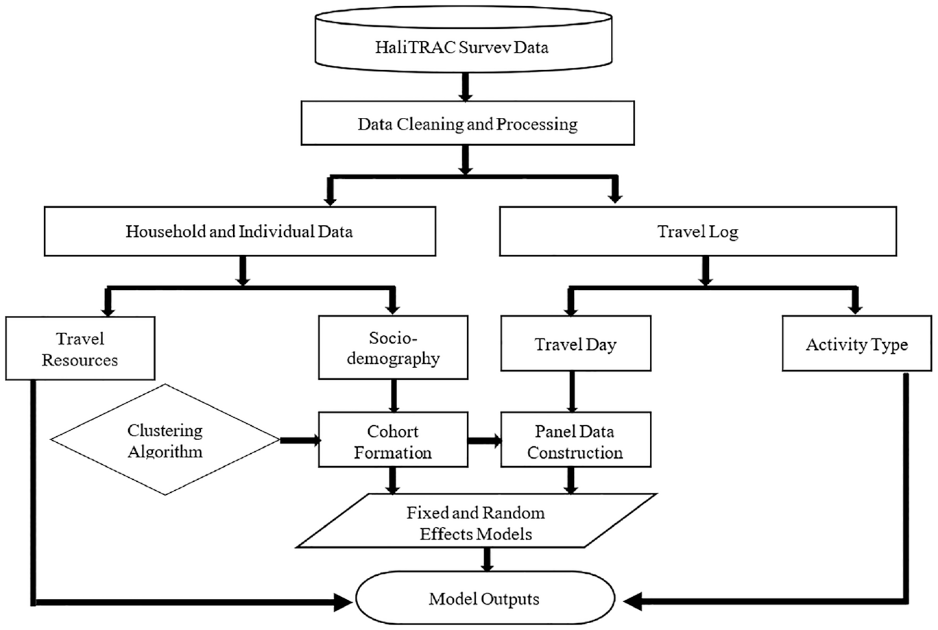
Process diagram of the research presented in this paper.
Descriptive Statistics of Respondents’ Demographic and Trip Attributes
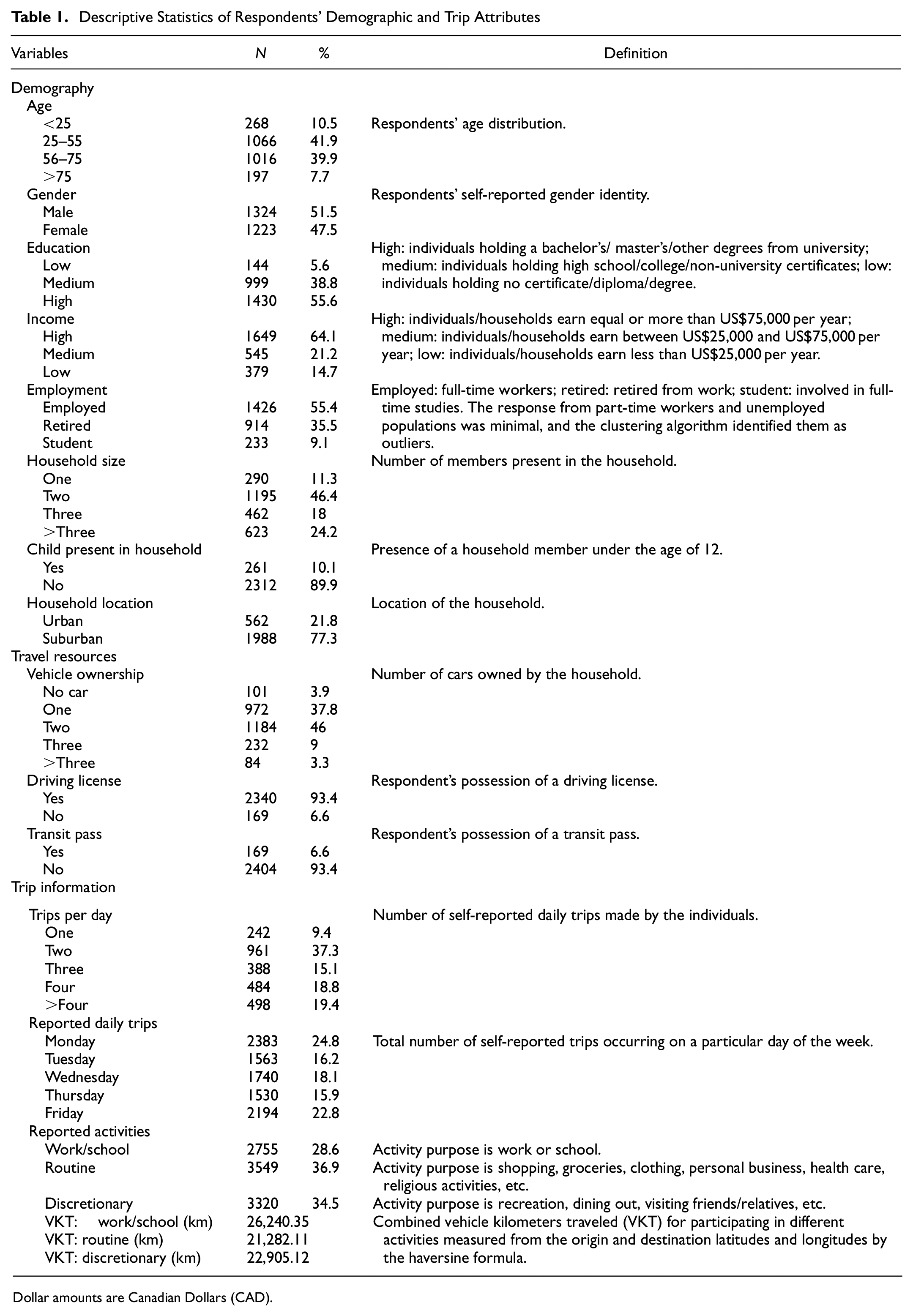
Dollar amounts are Canadian Dollars (CAD).
The representativeness of the sample considered in this study was evaluated by comparing sample data with the census 2021 data available on the Statistics Canada website ( 25 ). The socio-demographic variables age, gender, income, and employment were utilized for this purpose. The distribution of the attributes was found to align closely with the census data at 0%–7% variation. Therefore, the sample is considered representative of data for the population of HRM. Based on these conclusions, the dataset has not been weighted for further analysis. Figure 2 shows bar charts of the compared attributes.
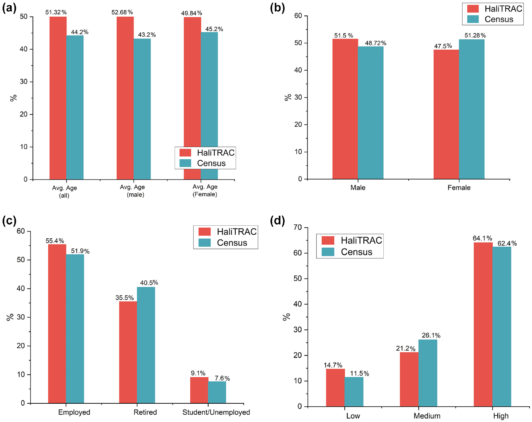
Comparison between HaliTRAC and census 2021 data: (a) age, (b) gender, (c) employment, and (d) income.
In this study, respondents’ activities were classified into three broad categories based on purpose: work/school, routine, and discretionary. This classification is drawn from previous research on activity participation and time allocation ( 26 – 28 ). For modeling, all variables in Table 1 were treated as independent variables, except for vehicle kilometers traveled (VKT), which served as the dependent variable for each activity category. The multivariate analysis estimated the impact of these variables on VKT for each activity.
Pseudo-Panel
Deaton’s ( 10 ) pseudo-panel method acts as a proxy for genuine panel data by forming observations from aggregation of cohorts. While individual observations are time-independent, once cohorts are created, they can be treated as a single observation with attributes spanning over time, similar to genuine panel data ( 29 ). A general mathematical formulation of the panel data regression model is shown in Equation 1:

Here,

Here, subscript
Dataset Construction
Similar to genuine panel data, a pseudo-panel dataset requires observations of a similar entity traced over a period of time. Given that cross-sectional data from various time periods contain observations of different individuals, aggregated observations are created based on distinct time-invariant characteristics. These observations are addressed as cohorts belonging to groups formulated in a way that large within-group similarity and between-group dissimilarity exist. Pseudo-panel dataset construction is highly data demanding and, to attain better model fit, a large cohort size along with a higher number of observations is required. A higher number of groups provides more observation but reduces the cohort size, and a large cohort size reduces the number of observations. Therefore, a balance needs to be identified between the size of cohorts and the total number of observations ( 31 ). Smaller cohort sizes can still yield better outcomes if the cohort construction process ensures maximum inter-group variation ( 29 ). This research employed an unsupervised machine-learning-based K-prototype clustering algorithm to form well-defined groups based on the four time-invariant socio-demographic variables age, gender, education, and employment. While previous research often used birth year as a common grouping factor ( 8 ), this study finds age more appropriate as a time-invariant factor because of the time variable being measured in days instead of years.
Huang’s (
32
) K-prototype clustering method was deemed most suitable because of its compatibility with both numerical (age) and categorical (gender, education, and income) data. The K-prototype algorithm for clustering begins by determining k centroids, represented as {C1, C2, ..., Ck} by selecting starting points on each variable {V1, V2, …, Vp}. It then proceeds to compute the distance between data points in the dataset and the centroids of the clusters, and subsequently assigns the data points to the cluster with the closest prototype distance to the centroid. After all objects have been allocated into clusters, the algorithm recalculates the new centroids of the clusters and reassigns all objects based on the updated prototypes. The error/cost function in the K-prototype measures the distance between the observed data points and the assigned prototype center. The mathematical formulation of cost minimization function for a mixed dataset

Here,
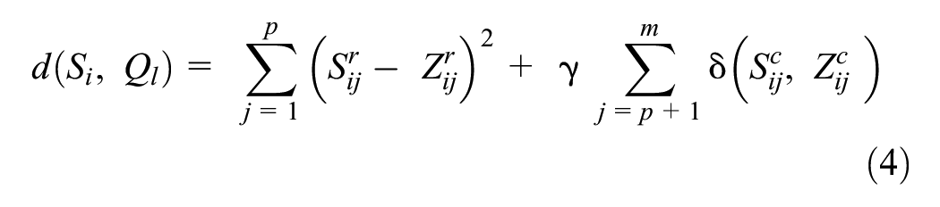
The first term of this equation measures squared Euclidean distance of the numeric values and the second term identifies dissimilarities of categorical data. Here,
Estimation Models
Estimating from pooled cross-sectional data often leads to biased estimates, primarily because of the presence of time-invariant unobservable variables correlated with the regressors. Models such as FE and RE control this bias by canceling it out or by considering it an exogenous factor. Tsai et al. ( 31 ) conducted a study to explore the performance of various estimation models on pseudo-panel data. Their findings revealed that the accuracy of the models is significantly influenced by the between- and within-group variance in the data, making it difficult to determine a definitive preferred model. Therefore, this research explored both static FE and RE models to identify the best fit.
Fixed Effects Model
The FE model has been largely used by researchers for static pseudo-panel estimation ( 8 , 12 , 17 , 36 ). This model adjusts against unobserved group effects by demeaning or subtracting the time-mean of each unit from its respective observations. By doing so, the pooled regression formula takes a reduced shape, as shown in Equation 5:

FE models are more flexible as they do not necessitate any specific assumptions with respect to the distribution of unobserved heterogeneity. However, in FE, the unobserved group effect varies over time, while the unobserved individual effect remains constant. Besides, the model focuses solely on within-group predictors, disregarding between-group differences. So, when there is significant variation in both within-group and between-group attributes, the accuracy of the FE estimation may be compromised ( 37 ).
Random Effects Model
The RE model, on the other hand, considers unobserved heterogeneity exogenous and unrelated to the explanatory variables. Since an entity’s error term is assumed to be uncorrelated with the regressors, time-invariant variables can also be considered independent variables. The model is estimated using the generalized least squares (GLS) or maximum likelihood (ML) methods, and it considers both between-group and within-group variations ( 12 ). The RE model is a hierarchical multilevel model and is especially suitable for research designs that involve data organized at multiple levels, that is, individuals and groups. However, if the assumption of exogenous unobserved heterogeneity is violated, the estimates may become biased.
Analysis and Results
The primary objective of this research was to develop a methodological framework for expanding single-day travel diaries to multi-day using a pseudo-panel approach. To achieve this, a series of comprehensive analyses were conducted. This section presents the systematic analysis approach along with its corresponding outcomes sequentially.
Cohort Formation and Dataset Construction
For cohort formation, four grouping criteria, age, gender, education, and employment, were chosen. Unsupervised K-prototype auto clustering was applied to the study sample using the IBM SPSS software tool. Auto clustering in SPSS determines the optimum number of clusters by monitoring changes in the Schwarz’s Bayesian information criteria (BIC) value. BIC serves as a measure of the prediction likelihood of the clustering model. When the optimal number of clusters is achieved, the BIC change becomes negligible, and the iteration process stops. In addition, the silhouette measure of cohesion and separation measure cluster quality based on data points’ similarity to their own cluster and dissimilarity to other clusters. Figure 3 demonstrates the optimum number of clusters and cluster quality from the analysis.
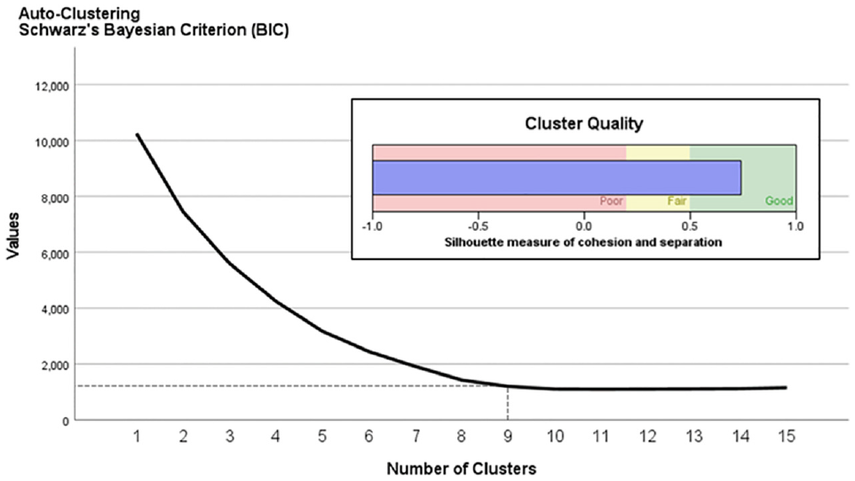
Optimum number of clusters and cluster quality from analysis.
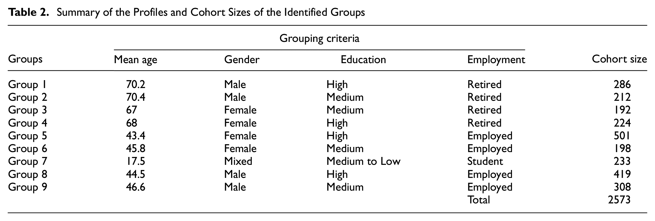
To adhere to the conventional terminology of pseudo-panel studies, clusters have been designated as groups, and individuals within these clusters have been referred to as cohorts from here onwards. Table 2 and Figure 4 present the profiles and cohort sizes of the groups derived from the analysis. The results identified four groups of retired-old males and females, four groups of working-class middle-aged males and females, and one group comprising young students with diverse genders and education levels.
Summary of the Profiles and Cohort Sizes of the Identified Groups
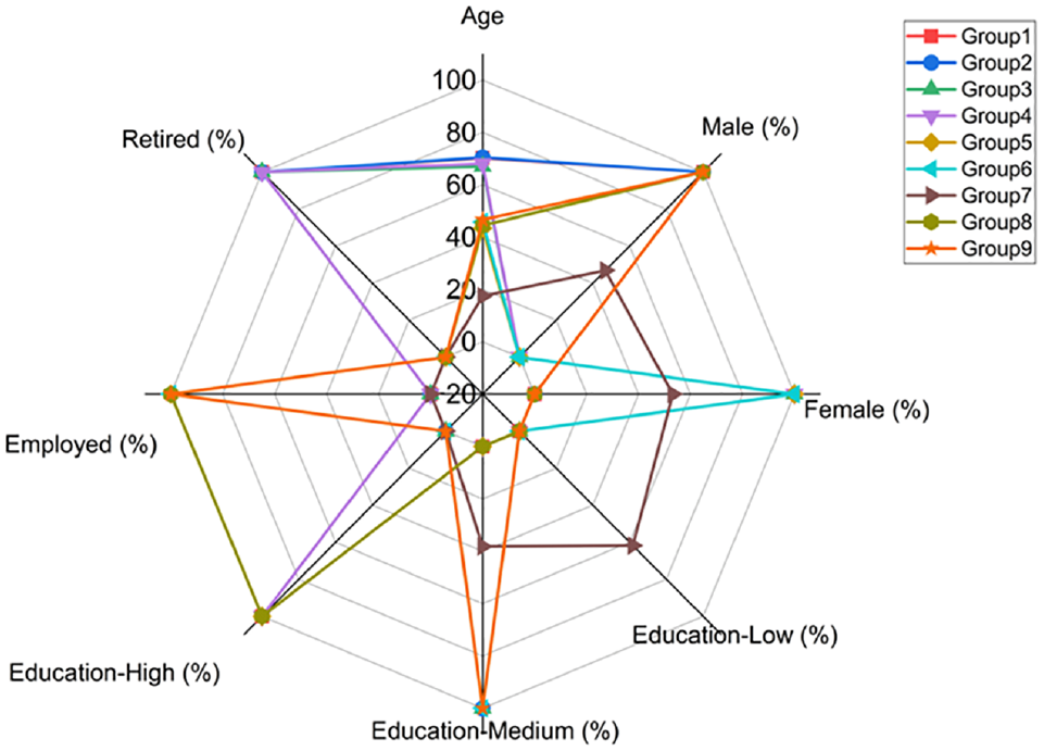
Cohorts’ socio-demographic characteristics.
It has been discussed earlier that the pseudo-panel dataset requires observations of similar entity traced over a period of time. Therefore, it is important that the systematically constructed observations (cohorts) exhibit their attributes at each time point. To satisfy this requirement, the formulated groups were re-evaluated based on the reporting days of cohorts’ travel diaries.
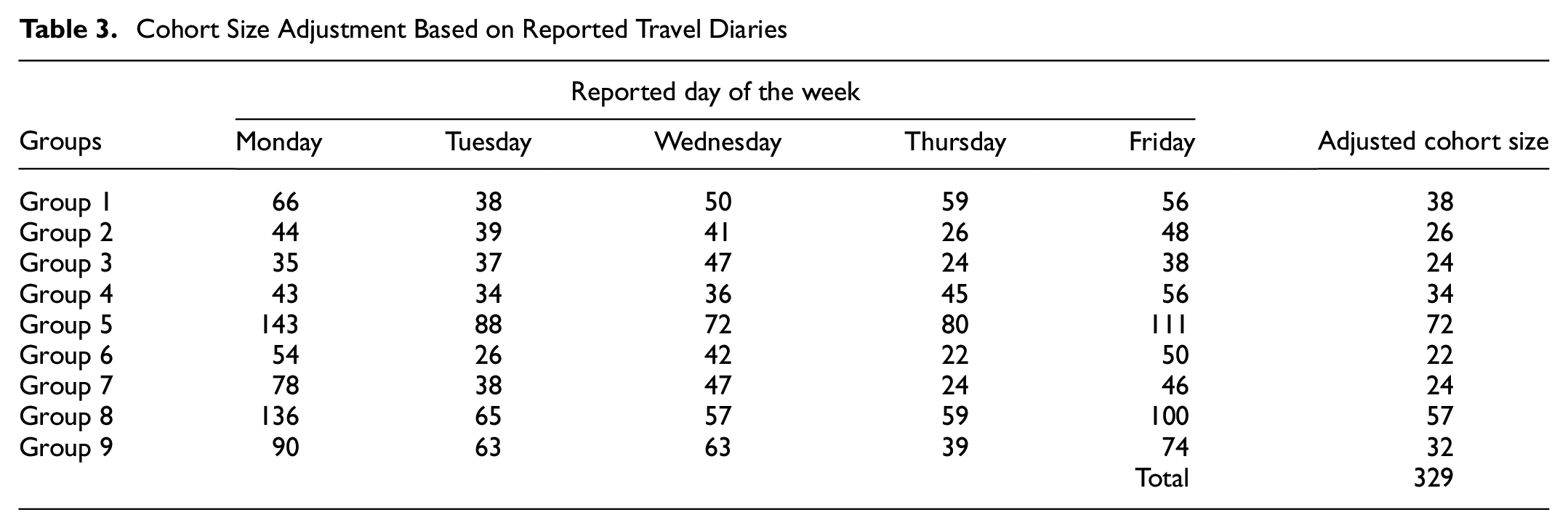
As seen in Table 3, cohort sizes have been adjusted based on the minimum number of 5e-day observations available for each group. Thus, 329 synthetic observations have been drawn from a pool of 2573 cohorts and were included in the pseudo-panel dataset for further analysis.
Cohort Size Adjustment Based on Reported Travel Diaries
Travel Pattern Analysis
The constructed pseudo-panel data constituted the cohort’s multi-day travel log. Therefore, several dynamic observations were made leveraging the longitudinal data format. The travel behavior of each group during weekdays was analyzed by dividing the total daily trips into hourly intervals. Noticeable dissimilarities in daily and hourly travel patterns across the groups were found. Figure 5 depicts the distribution of the trips and day-to-day variations. Groups 1–4, comprising retired-old males and females, exhibited a gradual increase in trips from late morning to a peak during mid-day, followed by a gradual decline in the evening. Their late evening trip count was observed to be relatively lower. Groups 5, 6 and 8, 9 were full-time workers and they exhibited two distinct morning and evening peaks, which are presumably work trips. Besides, they started trips earlier than the retired population and took part in a higher number of evening trips. With respect to day-to-day fluctuation of trips, working cohorts had higher fluctuations compared to the retirees. The student group also showed discernable characteristics in their travel pattern. For them, two distinct daily peaks were seen, the later peak occurring between noon and 3 p.m., considerably earlier than the working people’s evening peak. In general, there were significantly higher numbers of evening and late-night trips on Fridays among workers and students, but not among retirees.
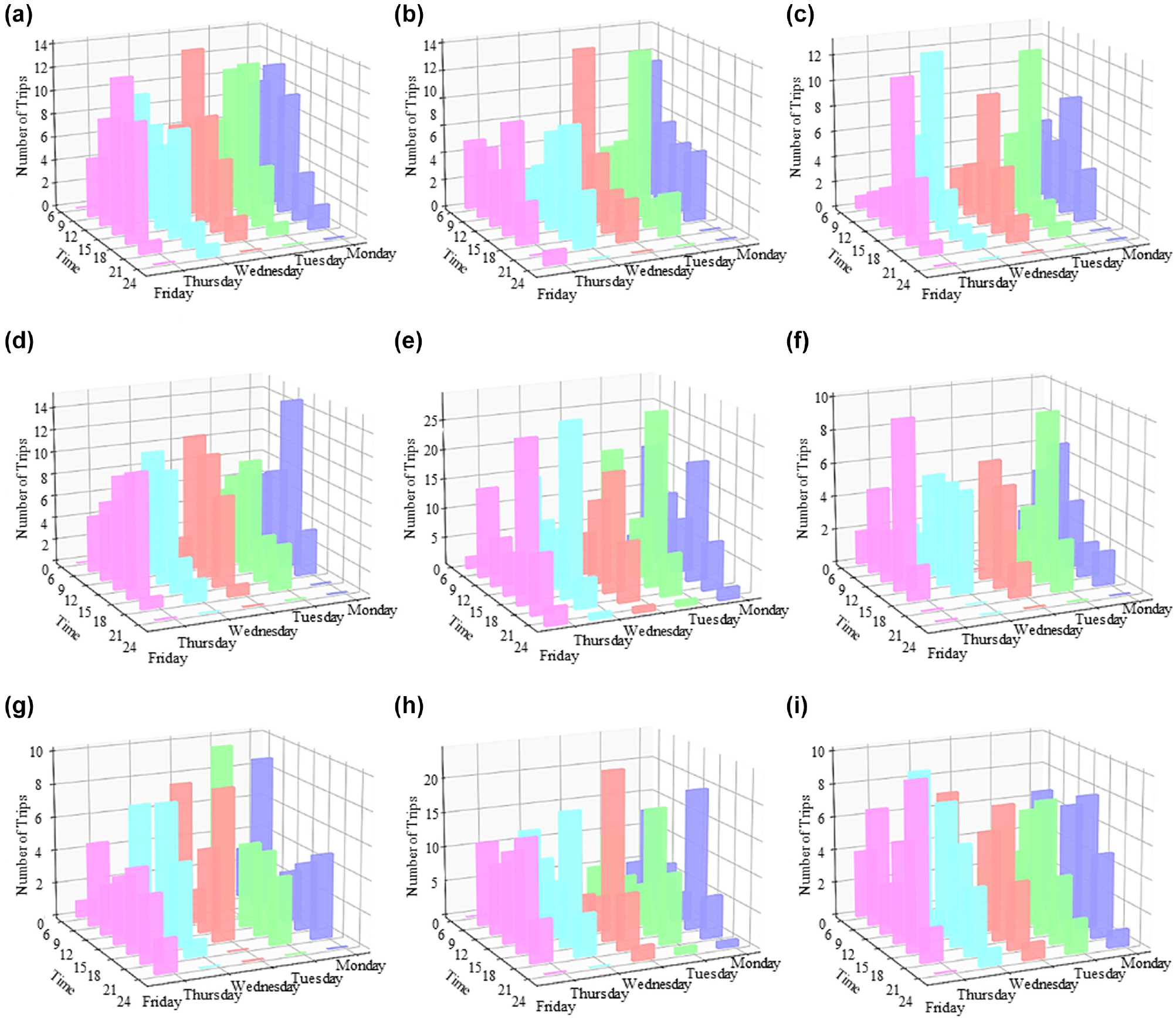
Daily and hourly distribution of the trips: (a) Group 1, (b) Group 2, (c) Group 3, (d) Group 4, (e) Group 5, (f) Group 6, (g) Group 7, (h) Group 8, and (i) Group 9.
Although disaggregated hourly and daily travel information provided interesting travel behavior inference, this study largely focused on cohorts’ weekday activity participation. Therefore, work/school, routine, and discretionary activities have been plotted in Figure 6 to examine the daily variation in activity participation across the groups. From the results, work or school trips were mostly observed for the employed and student groups. A “day of the week” effect was also discovered for work/school trips, since the number of trips gradually decreased from Monday to Friday. The highest numbers of individuals belonging to employed and student cohorts were found making work trips on Mondays, whereas the lowest number of trips were observed for Fridays.
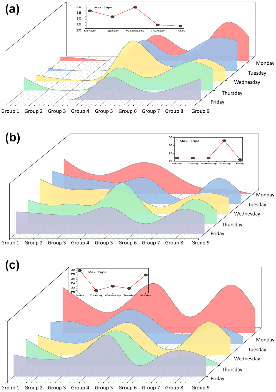
Daily variation in activity participation across the groups: (a) work/school, (b) routine, and (c) discretionary.
This outcome is most likely the effect of largely adapted hybrid/remote work and study arrangements in the post-pandemic periods. Routine activities, however, did not show significant temporal trend. However, a few important revelations were noted. Older cohorts were found to be more involved in routine activities, whereas young students were seen as less interested in it. Females took part more in routine activities compared to their male counterparts. Significant daily variations were observed in discretionary trips. Mondays and Fridays stood out as the days with the highest participation in discretionary activities, with Fridays being the most favored day. Older cohorts’ participation was considerably low compared to the middle-aged working people. Students, however, were found to be less involved in discretionary activities. From overall observation, students’ travel behavior seemed more restricted compared to the other groups, possibly because of reasons such as lacking a driving license, access to a car, or other necessary travel resources.
Model Implementation and Estimation
Based on the cohorts developed in this study, this paper utilizes FE and RE modeling techniques to gain a comprehensive understanding of the factors influencing activity participation. VKT to participate in three major activities, work/school, routine, and discretionary, was considered the continuous dependent variable. Thus, one FE model and one RE model were developed for each activity, yielding a total of six alternative models. The specification of the developed models is shown in Equation 6:
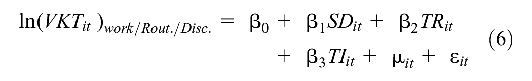
Here,
Estimates from the Work/School Activity Model
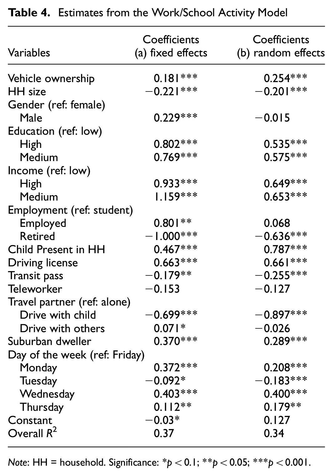
Note: HH = household. Significance: *p < 0.1; **p < 0.05; ***p < 0.001.
The findings from the work/school activity model revealed several intriguing insights. Most of the independent variables had a statistically significant influence on work/school VKT. Factors such as vehicle ownership, high income and education, employment, presence of children in the house, and driving license positively affected the dependent variable. Suburban dwellers were found to be traveling more for their work and school trips compared to urban dwellers. The study identified driving alone to work as the most favored travel arrangement, while teleworking and using public transit were found to be less favored for work/school-related purposes. Moreover, lengthier commutes for work or school were noted specifically on Mondays and Wednesdays, mirroring the observations depicted in Figure 6. A Durbin–Wu–Hausman (DWH) test was carried out to understand whether any correlation exists between the error terms and the regressors. The test results confirmed the correlation between unobserved effects and the independent variables. As a result, the FE model was considered more suitable for result estimation.
The next model also employed similar independent variables and modeling methods to estimate the determinants of routine activity participation. Table 5 illustrates the outcomes of the model.
Estimates from the Routine Activity Model
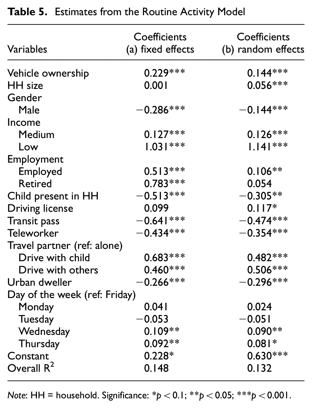
Note: HH = household. Significance: *p < 0.1; **p < 0.05; ***p < 0.001.
Factors such as vehicle ownership, household size, income, retirement, and driving license were found to be positively associated with routine VKT. Teleworkers and transit pass holders were found to travel less to participate in routine activities such as shopping, groceries, clothing, personal business, health care, and religious activities. In contrast to work and school trips, routine trips were frequently undertaken with partners or children, and males were less inclined to participate in routine activities. A significant temporal trend with respect to daily variation was not observed for routine activities. The model omitted a few observations because of collinearity and the DWH test identified the FE model, as more applicable as the assumption of variation across entities being random and uncorrelated did not hold true.
Table 6 illustrates the variables and their estimates for discretionary activity participation.
Estimates from the Discretionary Activity Model
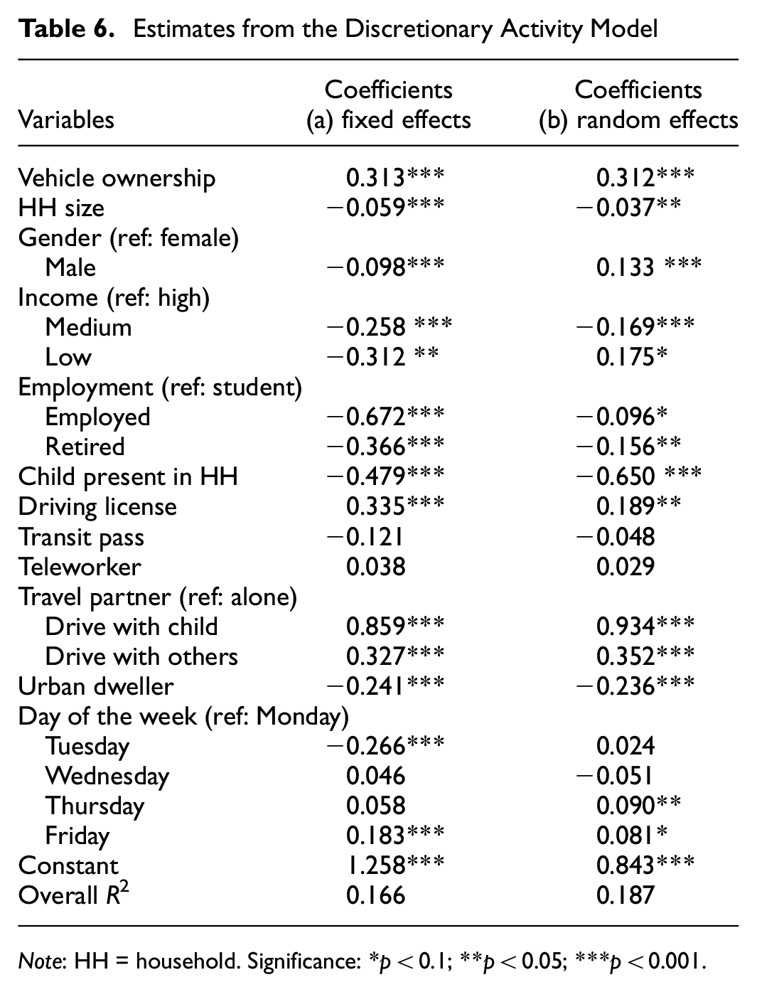
Note: HH = household. Significance: *p < 0.1; **p < 0.05; ***p < 0.001.
Results showed that vehicle ownership and driving licenses positively influence discretionary activities. Participation in discretionary activities was higher among retirees and employed individuals. Urban residents tended to travel shorter distances to engage in these activities. Having children and using public transit were identified as factors that decreased involvement in discretionary activities. It was observed that people often drove with their partners or children when attending such activities. In addition, the findings indicated that teleworkers had a higher likelihood of participating in these activities. A compelling temporal effect emerged, revealing that individuals are more inclined to extend their driving distances when engaging in discretionary activities, particularly on Fridays. Based on the DWH test, the RE model was determined to be a more suitable fit.
Conclusions and Policy Implications
This research aimed to develop a methodological framework for expanding single-day travel diaries to multi-day using a pseudo-panel approach and explore the temporal nexus in cohort-level activity participation. To achieve this, a data-driven clustering approach was followed for cohort formation and a time-series pseudo-panel dataset was constructed. Econometric estimation models were employed, and socio-demographic factors and travel resources-related determinants of activity participation were identified. Looking at the daily and hourly distribution of the trips, several interesting patterns were observed. The retired cohorts exhibited lower variation across the weekdays and a gradual mid-day peak. Their evening to after-hours trips were found limited. The worker and student cohort, on the other hand, showed two distinct a.m. and p.m. peaks with high travel variation across the weekdays. The p.m. peaks observed for the student cohorts occurred earlier than those for the workers. Work and school trips demonstrated a significant daily effect, as the number of trips gradually decreased from Monday to Friday. Older and female cohorts were found to be more involved in routine activities, whereas young students were seen to be less interested. Among the days of the week, Mondays and Fridays had the highest engagement in discretionary activities, with Fridays being the most preferred day. Activity participation was found to be largely attributed to vehicle ownership, income, education, driving license, and household structure. Possession of a transit pass not being positively associated with activities gives a hint of social exclusion faced by the transit users. This study also unveiled that teleworkers are more likely to take part in discretionary activities, as they are not burdened by mandatory or routine tasks. This notion has been supported in earlier studies also ( 3 , 38 ). In every instance of activity participation, it was observed that suburban residents tended to travel more than urban residents, indicating that mixed land-use developments lead to shorter trips and reduced VKT. The findings of this research call for policy re-evaluation to adjust and accommodate daily and hourly variations by optimal transit scheduling and route operation. Besides, by the detailed exploration and profiling of activities, participants can support decision-making that positively affects transportation, the environment, public health, and social well-being.
Limitations and Future Scope
There are several limitations and scope for future improvements. The aggregation effect on pseudo-panel data reduces individual-level heterogeneity, making nuanced observation of individual characteristics difficult. Also, because of limited data, static models were implemented overlooking the influence of the past day’s activities on the current day’s activity participation. Incorporating accessibility measures and factors related to the built environment has the potential to produce intriguing results in the proposed models. Future studies can investigate these shortcomings by collecting large samples of true panel data that can be implemented for both validation and dynamic model development. Nonetheless, this study offers a framework for analyzing travel patterns from a single-day data collection approach, where typical day assumptions are challenged given emerging post-pandemic travel behavior. This modeling approach will help to rethink multiple modeling aspects, including activity participation, scheduling, mode choice, shared travel, and destination choice models, within newer activity models that address the “typical weekday” barrier.
Footnotes
Author Contributions
The authors confirm contribution to the paper as follows: study conception and design: M.A. Habib, M.R.H. Bhuiyan; data collection: M.A. Habib; analysis and interpretation of results: M.R.H. Bhuiyan, M.A. Habib; draft manuscript preparation: M.R.H. Bhuiyan, M.A. Habib. All authors reviewed the results and approved the final version of the manuscript.
Declaration of Conflicting Interests
The author(s) declared no potential conflicts of interest with respect to the research, authorship, and/or publication of this article.
Funding
The author(s) disclosed receipt of the following financial support for the research, authorship, and/or publication of this article: This work was supported by a Natural Sciences and Engineering Research Council of Canada (NSERC) Discovery Grant, the Halifax Regional Municipality (HRM), and the Climate Action Awareness Fund (CAAF).