Sage Journals: Discover world-class research

Abstract

Mitotic count (MC) is an important element for grading canine cutaneous mast cell tumors (ccMCTs) and is determined in 10 consecutive high-power fields with the highest mitotic activity. However, there is variability in area selection between pathologists. In this study, the MC distribution and the effect of area selection on the MC were analyzed in ccMCTs. Two pathologists independently annotated all mitotic figures in whole-slide images of 28 ccMCTs (ground truth). Automated image analysis was used to examine the ground truth distribution of the MC throughout the tumor section area, which was compared with the manual MCs of 11 pathologists. Computerized analysis demonstrated high variability of the MC within different tumor areas. There were 6 MCTs with consistently low MCs (MC<7 in all tumor areas), 13 cases with mostly high MCs (MC ≥7 in ≥75% of 10 high-power field areas), and 9 borderline cases with variable MCs around 7, which is a cutoff value for ccMCT grading. There was inconsistency among pathologists in identifying the areas with the highest density of mitotic figures throughout the 3 ccMCT groups; only 51.9% of the counts were consistent with the highest 25% of the ground truth MC distribution. Regardless, there was substantial agreement between pathologists in detecting tumors with MC ≥7. Falsely low MCs below 7 mainly occurred in 4 of 9 borderline cases that had very few ground truth areas with MC ≥7. The findings of this study highlight the need to further standardize how to select the region of the tumor in which to determine the MC.

Keywords

area selection high-power field mitotic activity mitotic figure distribution tumor grading tumor periphery

Quantification of mitotic figures is one of the most common prognosticators of malignancy in veterinary and human tumor pathology.^25,26 It is well accepted that higher numbers of mitotic figures are commonly associated with a more aggressive behavior of neoplasms.^{14,15,18,34,38,47} Accurate quantification of mitotic figures in standard histological sections stained with hematoxylin and eosin (HE) has been shown to have higher correlation to prognosis than a subjective impression by quick scanning in human breast cancer.³⁹ Also for malignant neoplasms in veterinary pathology, it is recommended to routinely quantify mitotic activity by means of the mitotic count (MC), which is defined as the number of mitotic figures in 10 consecutive nonoverlapping high-power fields (hpf, field visible at 400× magnification with a field number [FN] of the ocular = 22, size = 2.37 mm²).²⁵ For some neoplasms (eg, canine mast cell tumors [MCTs],^20,30,43 canine and feline mammary tumors,^29,31 canine melanocytic tumors,⁴² or canine soft tissue sarcomas^13,24), the MC is also an important part of the tumor grading, and cutoff values for the MC have been established that directly affect tumor grade. For example, the canine cutaneous MCT (ccMCT) grading developed by Kiupel et al²⁰ uses a cutoff value of 7 mitotic figures in 10 hpf as one of the criteria to grade ccMCTs. Former grading systems have used the cutoff value of MC of 10.¹¹ Others have proposed prognostication of ccMCTs based entirely on the MC using a cutoff value of 5 or 7.^15,32

The MC is very applicable for routine surgical pathology and can be determined on glass and digital slides without any specialized equipment. Previous studies have shown that there is strong agreement in MC as determined by either light or digital microscopy in canine round cell tumors and human breast cancer.^1,7 Nevertheless, the MC has some limitations in terms of inconsistency between observers. Several studies on human breast cancer,^{1,9,12,27,28,44} canine mammary carcinomas,³⁶ and canine round cell tumors⁷ have shown that there is generally a high degree of interobserver and intraobserver variation of the MC. One of the most intensively discussed factors is the area unit “hpf,” which may vary up to 47% between different light microscopes at 400× magnification, depending on the FN of the respective ocular lens.^6,25 Surprisingly, many of the studies mentioned above did not define an hpf beyond being the field of view at 400× magnification. A standard FN of 22 mm with a subsequent area of an hpf at 400× magnification of 0.237mm² has been proposed for veterinary pathology by Meuten et al.²⁵ Similarly, when digital whole-slide images are viewed on a computer screen, the displayed area depends significantly on the monitor’s diagonal size.^7,25 Further attempts of standardization are to correct the MC by the proportion of neoplastic tissue within the hpf enumerated.¹² Indeed, standardization of the area size has been shown to somewhat improve concordance of the MC as has been demonstrated in canine round cell tumors with an increase of the concordance correlation coefficient by 0.044 (nonstandardized: 0.648; size standardized: 0.692) and human breast cancer with an increase of the coefficient of variance of 3.7% (56.0% in the conventional method and 52.3% in the volume-corrected method).^7,12

Another factor of influence is the difference between observers in their ability to identify individual mitotic figures and to distinguish them from other cell structures such as necrotic cells, especially in cases of prophase mitotic figures.^23,27,44 Few studies in human breast cancer reported only slight to moderate interobserver agreement (κ = 0.13–0.57) or 6.9% to 54.5% disagreement on deciding whether an individual cell structure represents a mitotic figure or not.^23,27,44 Appropriate sample fixation and slide preparation, including section thickness, are likely to have an impact on mitotic figure identification.⁶ The influence of the viewing modality (ie, light or digital microscopy) on identification of individual mitotic figures has not been fully assessed in veterinary or human pathology.

Importantly, selection of the evaluated hpf has been poorly standardized with vague selection criteria.^4,44 Therefore, we hypothesized that variable area selection may be another factor influencing the MC regardless of the tumor type. Most grading systems as well as general recommendations request that mitotic figures should be counted in a single area composed of 10 contiguous, nonoverlapping hpf located in the tumor region with the highest mitotic activity.* A tumor section with an area of 4.0 cm² contains more than 1600 nonoverlapping, standard-sized hpf. Therefore, scanning the tumor section and selecting the one area with the highest MC might be problematic.^4,44 Some studies circumvented this problem by counting mitotic figures in randomly selected hpf.^19,22,41 Others chose the most cellular or most anaplastic part of the tumor as well as excluding areas with necrosis, hemorrhage, and other artifacts.^6,13,24,25 It is also recommended to perform the MC in the periphery of the tumor as this is the invasive front and the most optimally fixed material.^6,25,26 Although there is no systematic study in veterinary pathology to date, some authors have hypothesized that the potentially more aggressive tumor cells with possibly more proliferation are located at the invasive front of the tumor.^25,37

In this study, we hypothesized that mitotic figures are not randomly distributed in ccMCTs and that an arbitrary selection of the area enumerated will influence the MC. To test this hypothesis, 2 pathologists annotated all mitotic figures in whole-slide images of HE-stained tissue sections of 28 different ccMCTs. Consecutively, a self-developed automated image analysis software was used to systematically analyze the distribution of mitotic figures throughout entire tumor sections (the software determined how many mitotic figures, which were labeled by 2 pathologists, were located in every possible 10-hpf area of the tumor; we did not use artificial intelligence to identify mitotic figures). MCs performed manually by 11 anatomic pathologists were compared with the computerized ground truth MC distribution to determine how successfully pathologists determine highest MCs. In addition, this study also tested the hypothesis that the density of mitotic figures is higher in the tumor periphery in comparison to the tumor center.

Materials and Methods

Specimens

Thirty-two ccMCTs, including 16 low-grade and 16 high-grade ccMCTs (2-tier grading system according to original diagnosis; all high-grade cases had a MC ≥7),²⁰ with acceptable tissue quality (determined by sufficient histological perceptibility of cellular details) were randomly selected from the authors’ archive. Subsequently, we excluded 4 cases with tumor section areas of <12 mm² from systematic analysis. These 4 ccCMTs contained very few mitotic figures (1 –5 mitotic figures in the entire tumor section with a highest possible MC of 1 or 2) and, therefore, were considered inappropriate for calculating MC distribution (exemplary heatmaps in Suppl. Figs. S1 and S2). MCTs had been formalin fixed, sectioned along their largest and orthogonal diameter, and paraffin embedded during routine diagnostic service. For this study, we produced new tissue sections of a single representative tissue block per case, which were subsequently stained with HE by a tissue stainer (ST5010 Autostainer XL; Leica, Wetzlar, Germany). All slides were digitalized with a linear scanner (ScanScope CS2; Leica) in 1 focal plane by default settings at a scanning magnification of 400×, resulting in an image resolution of 0.25 µm per pixel. Largest histopathological tumor diameters of the 28 cases were measured in the whole-slide image by the ruler tool of the Aperio ImageScope (Leica Biosystem Imaging) software and ranged from 5 mm to 28 mm (mean: 17.3 mm; Suppl. Table S1). Tumor diameters had to be determined from digitalized slides as gross measurements were not available for all cases. Statistical difference in largest tumor diameter between the later-defined 3 groups was calculated by a 2-sided t test by use of SPSS Statistics 25 for Windows (SPSS, Inc, an IBM Company, Chicago, IL).

Tumor Area and Mitosis Annotation

The open source software package SlideRunner² was used for 2 annotation tasks (Fig. 1A). First, mitotic figures were labeled within the entire whole-slide image by 2 pathologists (C.A.B., R.K.). Initially, the complete slide was screened twice for all mitotic figures within the tumor section by the first pathologist (C.A.B.). The screening was performed in a semiautomated manner, where the software would propose partly overlapping, consecutive image sections at a magnification of 400× to ensure that the entire whole-slide image was viewed thoroughly. As part of our annotation process, many of the nonmitotic cells (ie, mast cells, eosinophils, and other cell structures such as apoptotic cells) were annotated as a different annotation class. We considered this an important approach to reduce confirmation bias for the second annotation task. The second pathologist (R.K.) was then asked to assign a second class (ie, mitotic figure or nonmitotic cell) to all initially annotated structures, which were blinded to the cell class given by the first pathologist. This second opinion annotation was also performed in a semiautomated manner, where the software showed initial annotations that obscured the class previously assigned until all annotations on the slide had been given a second opinion. Both pathologists were instructed to only label convincing mitotic figures. Telophase figures with cytokinesis were labeled as a single mitotic figure. In total, 52 295 cell structures were annotated as mitotic figures by at least 1 of 2 pathologists in the 28 whole-slide images. Of those, 43 421 cells structures (83.0%) were agreed to be mitotic figures by both pathologists and were included in the ground truth data set for further analysis. Ground truth is a term for labeled data sets in image analysis that describes image information determined by the defined gold-standard method—in this case, the image location (coordinate) and annotation class (ie, mitotic figure) of manual annotations agreed on by both pathologists. For the remaining 8874 mitosis-annotations (17.0%), the 2 pathologists disagreed on whether or not the cell structure was a mitotic figure, and these annotations were disregarded for the following study. Furthermore, a total of 152 866 annotations were labeled as nonmitotic cell structures by consensus.

Figure 1.

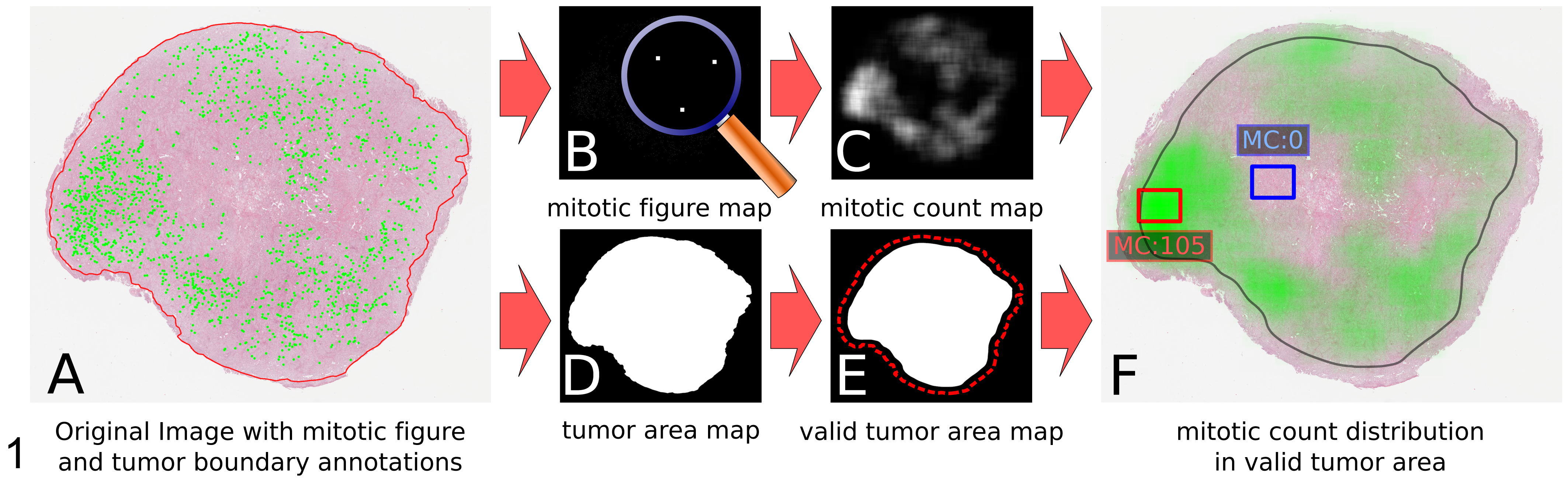
Overview of the processing chain to derive on-slide, ground truth mitotic count distribution from annotation data. (A) Original whole-slide image of a canine cutaneous mast cell tumor (hematoxylin and eosin [HE], case No. 20, group 3) with mitotic figure annotations (green dots) and tumor boundary annotations (solid red line). (B) Downsampled (reduction of the resolution) mitotic figure map derived from the mitotic figure annotations. (C) Mitotic count map representing the mitotic count determined within a defined area of 2.37 mm² (ie, 10 high-power fields [hpf]) for every possible center coordinate within the whole-slide image. Brighter colors show higher mitotic counts. (D) Downsampled, binary tumor area map derived from the tumor boundary annotations. (E) Valid tumor area map derived from the tumor area map excluding tissue in which the center coordinate of the 10-hpf area window would be covered less than 95% by tumor tissue. Original tumor boundary is depicted as a dashed red line. (F) Combined visualization of the whole-slide image (HE), the mitotic count map within the original tumor area (green overlay; higher opacity equals a higher mitotic count), and the valid tumor area indicated by a black line. The center of each 10-hpf area window was required to be within the black line. In this example, the mitotic count ranges from 0 (blue 10-hpf area window) to 105 (red 10-hpf area window).

Second, the tumor section area within the whole-tissue section was encircled by a single pathologist (C.A.B.) using a polygon annotation tool. This tumor area map included the entire tumor area and excluded necrotic areas; nontumor tissue within the tumor area larger than 1 hpf, such as a large blood vessel or entrapped residual tissue (sebaceous glands, hair follicles); and, in 1 case, a blurry image section (scanning artifact). In 3 cases (case Nos. 7, 16, and 22), there were areas within the tumor section area with variable cellularity.

Generation of the Mitotic Count Map

Computerized image analysis was used to determine distribution of the manually labeled mitotic figures within the valid tumor area. For this purpose, different image maps were created from ground truth mitotic figure and tumor area annotations. First, a size-reduced digital map of the ground truth mitotic figure annotations was created using a downsampling factor of 32 (Fig. 1B). In this binary mitotic figure map, the center of each mitotic figure was assigned the value “1” and other coordinates the value “0.” The result was a map that included all single mitotic events at their respective downsampled coordinates with reduced computational complexity over the typically very large original whole-slide image dimensions.

In a second step, we used a sliding window summation to assess the number of mitotic figures within a defined area in the slide. This tumor area was specified as a continuous region of adjacent 10 standard-sized hpf with each spanning 0.237 mm² as recommended by Meuten et al.²⁵ The resulting window covered a total area of 2.37 mm² with an aspect ratio of 4:3 centered on the respective coordinates and a width/height of 1777.6/1333.2 microns, or approximately 7110/5333 pixels at original scanning resolution, respectively. Downsampled as described above, the window was thus reduced to a size of 222 by 167 pixels. We decided to use the shape of a 4:3 rectangle for the 10-hpf area, as the viewing area of digital microscopy (computer screen) is rectangular, not round, as for light microscopy. For each pixel position of the downsampled mitotic figure map, a frame of that defined size was centered on this pixel position, and the sum of all mitotic figures within that frame was calculated. This sliding window summation yielded the mitotic count map that contained every possible mitotic count given an arbitrary center coordinate of the 10-hpf area (Fig. 1C). In other words, a pixel of the mitotic count map represents the MC within the 10-hpf area of which it is the center coordinate. Those steps described above have been replicated for defined areas of 20 hpf (4.74 mm²) and 50 hpf (11.85 mm²).

Generation of the Valid Tumor Area Map

In a next step, a map of the valid tumor area in the tissue section was created as the region on the whole-slide image in which the MC derived from the mitotic count map had to be determined. We took the annotated area of tumor tissue on each slide and removed all exclusion image parts representing nontumor tissue, necrotic tumor tissue, and blurry image regions. This resulted in a tumor area map, in which the entire tumor tissue was represented by the value “1” and all nontumor tissue by “0” (Fig. 1D). The size of the tumor section area was determined from this map. The selected tumor sections had a mean tumor section area of 167.86 mm² (range: 14.86–346.10 mm²; standard deviation: 95.01 mm²; see Suppl. Table S1 for tumor size of individual sections).

Subsequently, a derived valid tumor map was created that comprised all coordinates in which the center coordinate of the 10-hpf, 20-hpf, and 50-hpf area was placed while covering tumor tissue (tumor area map) by at least 95% of the hpf area (Fig. 1E). To achieve this, we used a moving window averaging approach with a subsequent threshold of 0.95, effectively yielding a valid tumor map with reduced area over the initial tumor area map.

Computerized Analysis of the Ground Truth MC Distribution

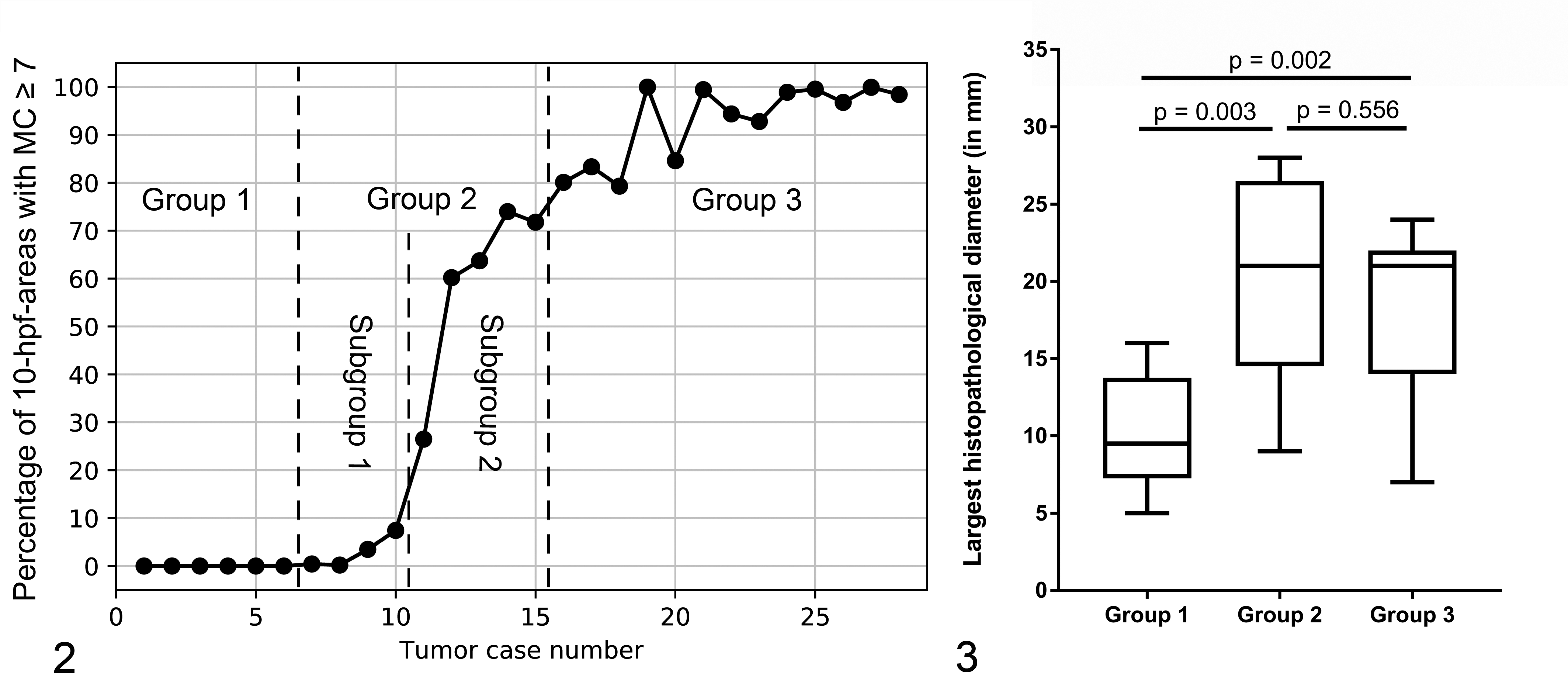
For statistical analysis, all entries of the mitotic count map that were valid as per valid tumor area map were considered. Depending on the size of the valid tumor area, the total amount of 2.37-mm² area windows evaluated varied from 57 665 to 4 185 973 between the 28 cases (Suppl. Table S1). These numbers included all possible pixel positions of the 2.37-mm² area window within the downsampled valid tumor area that was determined by computerized calculation and used for the ground truth MC distribution. First, we computed the probability to arbitrarily select a high MC (MC ≥7) 10-hpf area—that is, the number of the 10-hpf areas that contained equal to or more than 7 mitotic figures divided by all possible 10-hpf areas within the valid tumor area (without exclusion tissue). The likelihood to select low MC areas (MC <7) is the reciprocal of the indicated values. Based on that determined probability of the ground truth MC being above the cutoff value of 7, we defined 3 groups of ccMCTs (Fig. 2): (1) group 1 (low MCs, n = 6) has a 0% ground truth probability of a MC ≥7 (ie, all potential contiguous 10-hpf areas have MCs <7), (2) group 2 (borderline cases, n = 9) has a 0.01% to 74.99% probability of selecting an area with a MC above the cutoff value of 7 (ie, at least contains one 10-hpf area with MC ≥7), and (3) group 3 (mostly high MCs, n = 13) has a ≥75% ground truth chance of arbitrarily selecting an area that has a MC ≥7 (ie, mostly comprises 10-hpf areas with MC ≥7). In addition, we similarly evaluated 2 further published cutoff values of 5 and 10.^11,20,32 Second, we determined the regional variability of the mitotic count of each case by heatmaps, box-and-whisker plots (see Suppl. Table S2 for minimum, first quartile, median, third quartile, and maximum value), and histograms. Heatmaps were generated by adding a semitransparent green overlay to the microscopic image with the maximum value (as indicated by the color bar) having no transparency and the minimum value having full transparency (transparency is relative to the maximum MC). Box-and-whisker plots and histograms were generated with the python matplotlib 2.2.2 software (open source software, from www.python.org). Effects of cellular density were determined subjectively based on the heatmaps.

Figures 2–3. Comparison of the 3 canine cutaneous mast cell tumor groups that were defined as follows: group 1 (uniformly low mitotic count [MC]), group 2 (borderline, with subgroups 1 and 2), and group 3 (mostly high MC). Figure 2. Ground truth percentage of 10 high-power field (hpf) areas with a MC ≥7 relative to the total number of all possible 10-hpf areas within the section. The 3 black broken vertical lines separate the defined groups and subgroups. The percentage of 10-hpf areas with MC <7 is the reciprocal of the indicated values. Figure 3. Comparison of the largest histopathological tumor diameter among the 3 tumor groups. The boxes show the first quartile, second quartile (median), and third quartile; the whiskers show the range (minimum and maximum) of the data. There is a significant difference (P < .05) between groups 1 and 2 as well as groups 1 and 3.

Manual MC by Pathologists

Manual mitotic counts were obtained according to current guidelines by 11 board-certified anatomic pathologists (A.S., C.G., D.G.S., E.L.N., M.D., M.K., O.K., R.K., R.C.S., S.M.C., T.T.; order of participants has been randomized for analysis) from 4 different diagnostic laboratories by examining the same digital images that were used for the ground truth data set. Pathologists were instructed to perform the MCs in the area with the highest mitotic density as requested by the current grading system to simulate a diagnostic setting.²⁰ According to current recommendations, the number of required hpf was calculated for each pathologist to examine a total area of 2.37 mm², as the size of a hpf varies between different computer monitors.²⁵ Presentation order of the 28 cases was randomized. Pathologists were blinded to the tumor grade and the MCs of other pathologists. A total of 308 MCs were available as a result of 11 pathologists examining all 28 cases (Suppl. Table S3). The MCs of the pathologists were categorized using the quartiles of the ground truth MC distribution. We chose a classification in favor of the pathologists by defining the categories as greater than or equal to the lower bound quartile. Following this rule, the categories were defined as follows: category 1 (MCs < first quartile), category 2 (first quartile ≤ MCs < median), category 3 (median ≤ MCs < third quartile), and category 4 (third quartile ≤ MCs). Low MC (group 1) cases had a very narrow ground truth distribution with close to equal quartile cutoff values (discrete counts), and therefore category 4 may include significantly more than 25% of the values. Categories 3 and 4 combined represent the highest 50% of all possible ground truth MCs. In addition, we categorized the MCs into below and above the cutoff value for ccMCT grading/prognostication.^11,15,20,32 The 95% confidence intervals (CIs) were determined by the Wilson method with a continuity correction. Agreement for the high MC classification (MC ≥7) was evaluated by Light’s κ for fully crossed designs, and interrater agreement for the raw MC values of all pathologists was evaluated by the intraclass correlation coefficient (ICC; 2-way agreement, single measures, random). The κ and ICC values are measures of the level of agreement corrected by chance between different participants; however, they do not indicate degree of accuracy to the ground truth. We evaluated κ as poor = 0, slight = 0.01–0.20, fair = 0.21–0.40, moderate = 0.41–0.60, substantial = 0.61–0.80, and almost perfect = 0.81–1.00.¹⁷ ICC was evaluated as poor = 0–0.39, fair = 0.40–0.59, good = 0.6–0.74, and excellent = 0.75–1.00.¹⁷ Calculations were performed using R version 3.52 (R Foundation, Vienna, Austria) using the package irr version 0.84.1.¹⁶

Differences Between Tumor Periphery and Center

Counting mitotic figures at the periphery of the tumor section has been recommended due to better fixation and suspected higher proliferation of tumor cells at the invasion front.²⁵ For this reason, the ground truth mitotic activity index (MAI) was compared between the tumor periphery and center. MAI is defined as the number of mitotic figures within a tumor area, in this case tumor periphery or center, divided by the size (in mm²) of that respective area.²⁵ As there is currently no consensus on the proportional and absolute size of the periphery in ccMCTs, we evaluated 3 different ratios of the tumor periphery containing 25%, 50%, and 75% of the total tumor area, respectively. The tumor periphery was defined as the area between the tumor border margins, which was annotated by a single pathologist (see above), subtracted by the area of the tumor center, which was determined by stepwise reduction of the tumor area from the outside (erosion operator with uniform 3 × 3 filter kernel) until the target percentage of 75%, 50%, and 25% (standard deviation: <0.15%) was reached. Tissue sections that contained widespread necrosis and ulceration, nontumor tissue, and scanning artifacts were excluded from calculation as described above. If the whole-slide image comprised several tissue sections, area proportions were determined for the joint area of the sections, and calculations of tumor size and MAI were added. Differences of the MAI between periphery and center for each defined proportion were tested for significance by a 2-sided t test with the python scipy version 1.1.0 stats-package software.

Results

Probability of Assigning High MC in Arbitrary Area Selection

The ground truth chances to arbitrarily select a tumor area that contains MCs above the cutoff value of MC ≥7 ranged from 0% to 99.97% (Suppl. Table S4). Group 1 (always low MC, 0% chance) contained 6 ccMCTs (case Nos. 1–6) and had the significantly (P ≤ .003) smallest histopathological tumor diameters, ranging from 5 to 16 mm (median: 9.5 mm; Fig. 3). Group 2 (borderline cases) included 9 ccMCTs with a very small (0.20%–7.43%; case Nos. 7–10; subgroup 1) to moderate (26.48%–73.97%; case Nos. 11–15; subgroup 2) ground truth chance of arbitrarily selecting a high MC area. In other words, these cases included few (subgroup 1; third quartile below 7) to numerous (subgroup 2; third quartile equal to or greater than 7) tumor areas with a MC ≥7, and they included many tumor areas with a MC <7. In group 2, largest histopathological tumor diameters ranged from 9 to 28 mm (median: 21 mm) and were significantly (P = .003) larger than for group 1 MCTs, while 2 cases (case Nos. 9 and 10) had smaller tumor diameters than the maximum tumor diameter of group 1 MCTs (Fig. 3). Group 3 (mostly high MC, ≥75% chance) comprised 13 ccMCTs (case Nos. 16–28). In group 3, the largest tumor diameters of histopathological sections ranged from 7 to 24 mm and were overall significantly (P = .002) larger than tumor diameters of group 1 MCTs. However, 3 cases (case Nos. 19, 21, and 25) overlapped with the tumor diameter range of group 1 MCTs (Fig. 3). Although in most cases, the MC range correlated with the tumor diameter, case Nos. 19, 21, and 25 were noteworthy exceptions.

Ground Truth MC Distribution

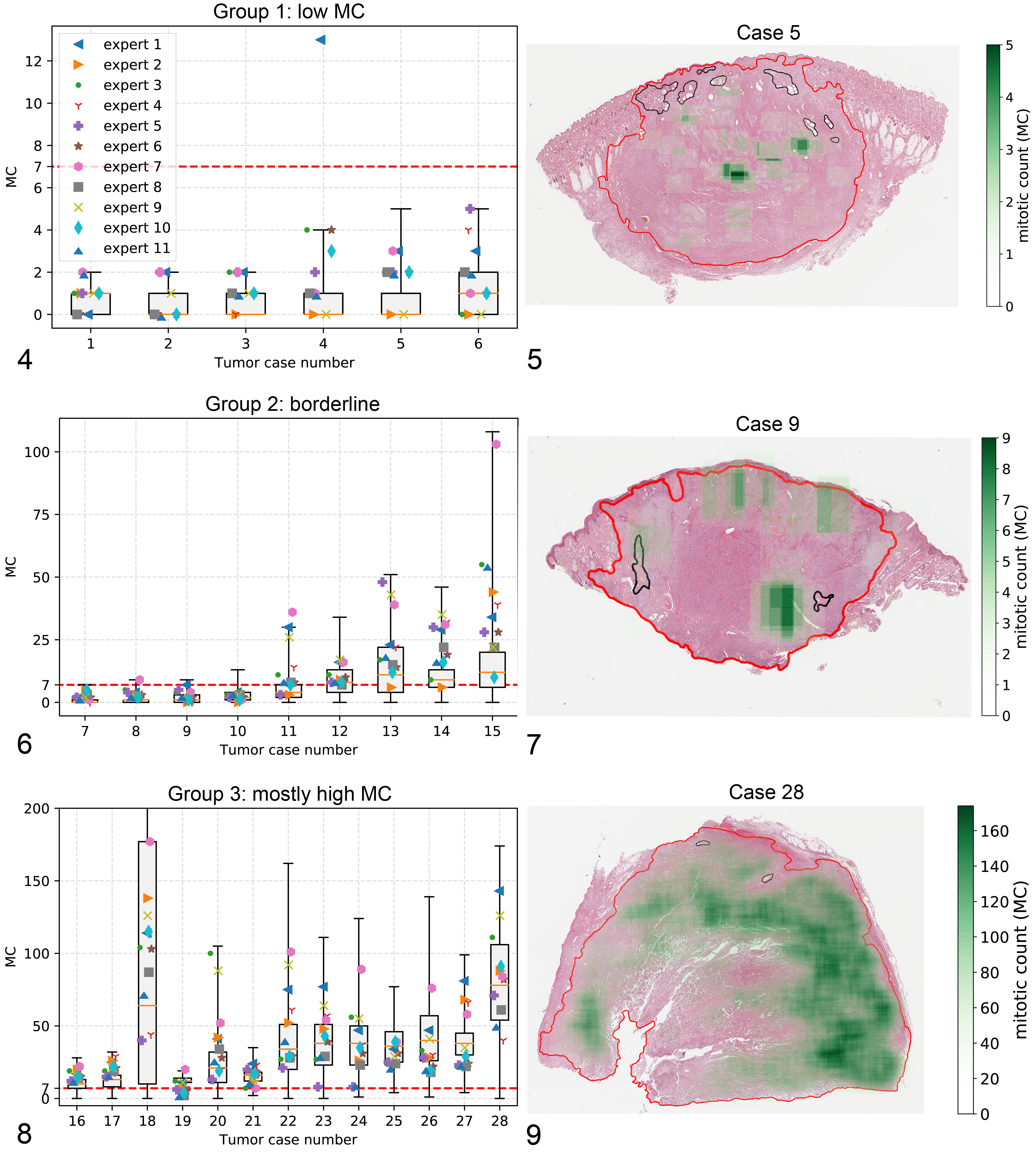
Ground truth mitotic figures were irregularly distributed throughout the tumor section area for all groups—that is, there were different MCs depending on the tumor region assessed (Suppl. Figs. S1 and S2). Always low MC cases (group 1) had MC ranges between 0 and 5 (Figs. 4, 5). Therefore, area selection seems to be of minor importance in this group. Borderline cases (group 2; Fig. 6) had lower MC ranges in subgroup 1 between 7 and 13 (Fig. 7) compared to subgroup 2 with MC ranges between 30 and 108 (Suppl. Fig. S3). In contrast to group 1, area selection seems to be essential in group 2. Mostly high MC cases (group 3) had the highest ground truth MC between 28 and 335 (Figs. 8, 9). In this group, random area selection would rarely lead to MCs below the cutoff value. Case No. 19 had an exceptionally narrow distribution, and this tumor also had the smallest size. The present study included 3 ccMCTs with distinctly variable cellular density throughout the tumor section. Whereas in 1 case, the highest mitotic counts were in areas with high cellular density (case No. 18; Suppl. Fig. S4), another case had the highest activity in a region with low cellular density (case No. 7; Suppl. Fig. S5). In the third case, cell-sparse regions had medium mitotic activity (case No. 22; Suppl. Fig. S6).

By increasing the size of the area examined (10 hpf to 20 hpf and 50 hpf), the range of MC distribution (maximum and minimum) was generally mildly to moderately reduced (Suppl. Figs. S7–S9), and the highest MC value was lowered to beneath the cutoff value in case Nos. 7 to 10 (all cases of subgroup 1 from the borderline group). However, the median values largely remained unchanged.

Pathologist’s Manual MC

Overall interobserver agreement of the manual MCs of 11 board-certified pathologists was good (ICC = 0.715; CI, 0.592–0.830). In comparison, the ICC of group 3 was smaller (ICC = 0.603; CI, 0.402–0.816), indicating that agreement on the highest values becomes more difficult with higher MC ranges. ICCs of other groups are not indicated since the range of possible values was quite small and relative deviation was therefore overinflated (ICC values were quite small and should not be interpreted as such).

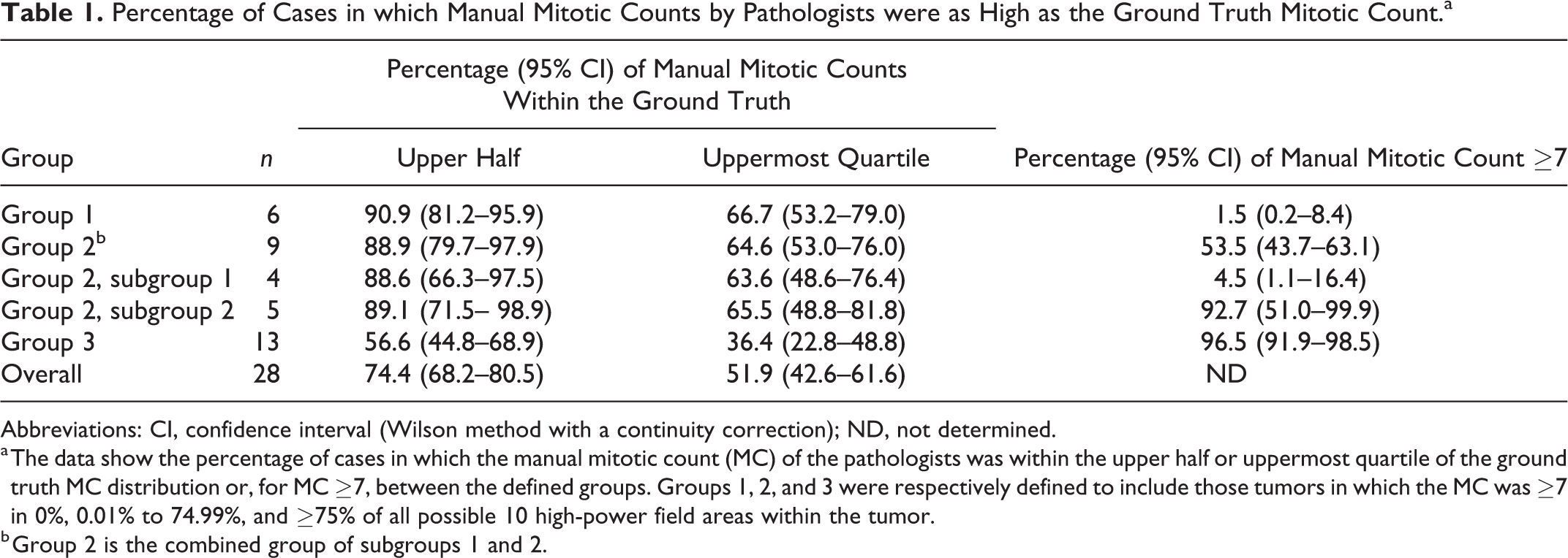
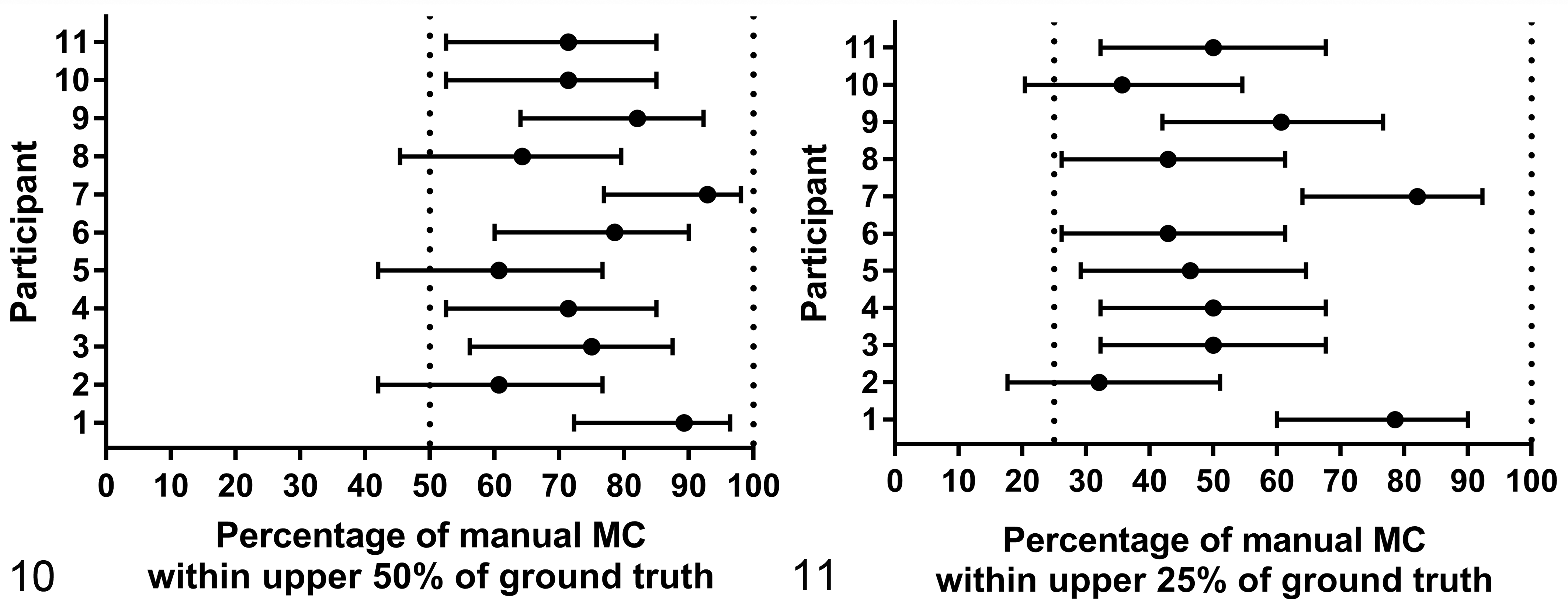
Compared to the ground truth distribution, the manual MCs ranged from low to high values (Figs. 4, 6, 8). Of all manual counts of all pathologists, 74.4% (CI, 68.2%–80.5%) were within the highest ≥50% (categories 3 and 4) of all ground truth MCs and 51.9% (CI, 42.6%–61.6%) were within the highest ≥25% (category 4) (Table 1, Suppl. Fig. S10). Manual MCs of MCTs in group 3 were less often within the highest half (56.6%; CI, 44.8%–68.9%) and quarter (36.4%; CI, 22.8%–48.8%) of all possible ground truth MCs in comparison to group 1 (within highest half in 90.9% [CI, 81.2%–95.9%]; within highest quarter in 66.7% [CI, 53.2%–79.0%]) and group 2 (within highest half in 88.9% [CI, 79.7%–97.9%]; within highest quarter in 64.6% [CI, 53.0%–76.0%]). When comparing the individual pathologists, there was high variability between MCs being within the ground truth highest half ranging from 60.7% to 92.9% (Fig. 10, Suppl. Table S5) and highest quarter ranging from 32.1% to 82.1% (Fig. 11, Suppl. Table S5).

Figures 4–9. Distribution of ground truth mitotic counts (MC) among 28 histopathological sections of canine cutaneous mast cell tumors. Figures 4, 6, and 8. Box-and-whisker plots (boxes show the first, second, and third quartiles; whiskers show the minimum and maximum of the data) of the ground truth MC distribution of individual cases, divided into group 1 (uniformly low MCs; Figure 4), group 2 (borderline MCs; Figure 6), and group 3 (mostly high MCs; Figure 8). The cutoff value for tumor prognostication (MC ≥7) is indicated by the red dashed line. Absolute numbers of the manual MC performed by 11 pathologists are indicated by the different symbols in the individual boxplots. Figures 5, 7, and 9. Exemplary cases of the 3 tumor groups, including case Nos. 5 (Figure 5; low MC), 9 (Figure 7, borderline), and 28 (Figure 9, mostly high MC). The images show the whole-slide image (hematoxylin and eosin) of the respective case with tumor border annotations (red lines) and the ground truth heatmap of the MC as a green overlay with a MC range indicated by different opacity (scale on the right side).

Table 1.

Percentage of Cases in which Manual Mitotic Counts by Pathologists were as High as the Ground Truth Mitotic Count.^a

Group	n	Percentage (95% CI) of Manual Mitotic Counts Within the Ground Truth		Percentage (95% CI) of Manual Mitotic Count ≥7
Group	n	Upper Half	Uppermost Quartile	Percentage (95% CI) of Manual Mitotic Count ≥7
Group 1	6	90.9 (81.2–95.9)	66.7 (53.2–79.0)	1.5 (0.2–8.4)
Group 2^b	9	88.9 (79.7–97.9)	64.6 (53.0–76.0)	53.5 (43.7–63.1)
Group 2, subgroup 1	4	88.6 (66.3–97.5)	63.6 (48.6–76.4)	4.5 (1.1–16.4)
Group 2, subgroup 2	5	89.1 (71.5– 98.9)	65.5 (48.8–81.8)	92.7 (51.0–99.9)
Group 3	13	56.6 (44.8–68.9)	36.4 (22.8–48.8)	96.5 (91.9–98.5)
Overall	28	74.4 (68.2–80.5)	51.9 (42.6–61.6)	ND

Abbreviations: CI, confidence interval (Wilson method with a continuity correction); ND, not determined.

^a The data show the percentage of cases in which the manual mitotic count (MC) of the pathologists was within the upper half or uppermost quartile of the ground truth MC distribution or, for MC ≥7, between the defined groups. Groups 1, 2, and 3 were respectively defined to include those tumors in which the MC was ≥7 in 0%, 0.01% to 74.99%, and ≥75% of all possible 10 high-power field areas within the tumor.

^b Group 2 is the combined group of subgroups 1 and 2.

Figures 10–11. Forest plots of the manual mitotic count (MC) being above or equal to the upper half or upper 25%, respectively, of ground truth MC distribution comparing the 11 pathologists. Of each graph, the central symbol represents the result of the respective participant, and the attached line represents the confidence interval (Wilson method with continuity correction). The left dotted lines demarcate the chance if the 10 high-power field (hpf) areas were selected randomly (50% and 25%, respectively), and the right line indicates the ideal achievement (100%). Figure 10. Forest plot of the MC being above or equal to the ground truth median. Chance in fully random area selection would be 50%. Figure 11. Forest plot of the MC being above or equal to the ground truth third quartile. Chance in fully random area selection would be 25%.

In addition, we tested whether the manual MCs were above or below the grading cutoff of 7 (Suppl. Fig. S11). Overall, there was substantial agreement between pathologists to detect high MCs above or equal to 7 (κ = 0.865) for all cases combined. When comparing the 3 tumor groups, the MCs resulted consistently in a good prognosis and poor prognosis designation (based on the MC alone) for ccMCTs in groups 1 and group 3, respectively. However, for the borderline group, the MC was variable around the cutoff value, which would potentially affect the assigned grade. In low MC cases (group 1), the manual MCs were below 7 in 98.5% (CI, 91.6%–99.8%; 1.5% false positive) with only 1 overestimated count (case No. 4). In group 3 ccMCTs, pathologists determined MCs ≥7 with a detection rate of 96.5% (CI, 91.9%–98.6%; mean ground truth chance in random area selection is 92.9%) with disagreement only in case No. 19, which had a very narrow distribution. Manual MCs of borderline cases, which contained at least 1 area with MC ≥7 according to the ground truth distribution, were above the cutoff only in 53.5% (95.5% CI, 43.5%–63.3%; mean ground truth chance in random area selection is 34.2%). In this group, underestimation of the MCs mainly occurred in subgroup 1, which had the cutoff value of 7 in the upper quartile of the ground truth distribution. Detection rate for MC ≥7 was 4.5% (CI, 1.1%–16.4%; mean ground truth chance in random area selection is 2.9%). In contrast, pathologists had a detection rate of 92.7% (CI, 51.0%–99.9%) for MC ≥7 for subgroup 2 cases (case Nos. 11–15; ground truth chance above 25%; mean is 59.2%); that is, they consistently reached cutoff values.

Usage of Different Cutoff Values

We tested the influence of various published cutoff values (ie, MC ≥ 5, MC ≥7, and MC ≥10).^11,15,20,32 Compared to the commonly used cutoff value of 7, we found considerable differences in the probability to assign a prognosis, with cutoff values of 5³² leading to a higher chance and cutoff values of 10¹¹ leading to a lower chance of assigning a poor prognosis/outcome (Suppl. Figs. S11, S12 and Suppl. Table S4). The influence was most significant in the borderline cases (group 2), with the greatest difference in chance between the cutoff values of MC ≥5 and MC ≥10 being 42.56% in the most extreme case (tumor case No. 14; mean difference: 20.5%). There was a mean difference of 0.04% (range: 0.00%–0.18%) in group 1 and a mean difference of 9.09% (range: 0.28%–38.66%) in group 3. Similar effects were observed with the manual MCs performed by the 11 pathologists (Suppl. Table S4). Based on the manual MCs, borderline cases would have been assigned a high grade in 59.6%, 53.5%, and 33.3% (a difference of 26.3%) by the cutoff values of 5, 7, and 10, respectively. Therefore, the usage of different cutoff values resulted in relevant interobserver variation for borderline cases. On the other hand, group 1 cases had a difference of only 1.5% (3.0%, 1.5%, and 1.5% probability, respectively), and group 3 cases had a difference of only 4.6% (97.9%, 96.5%, and 93.3% probability, respectively). As such, the cutoff value applied had minimal impact on interobserver variation.

Differences Between the Tumor Periphery and Center

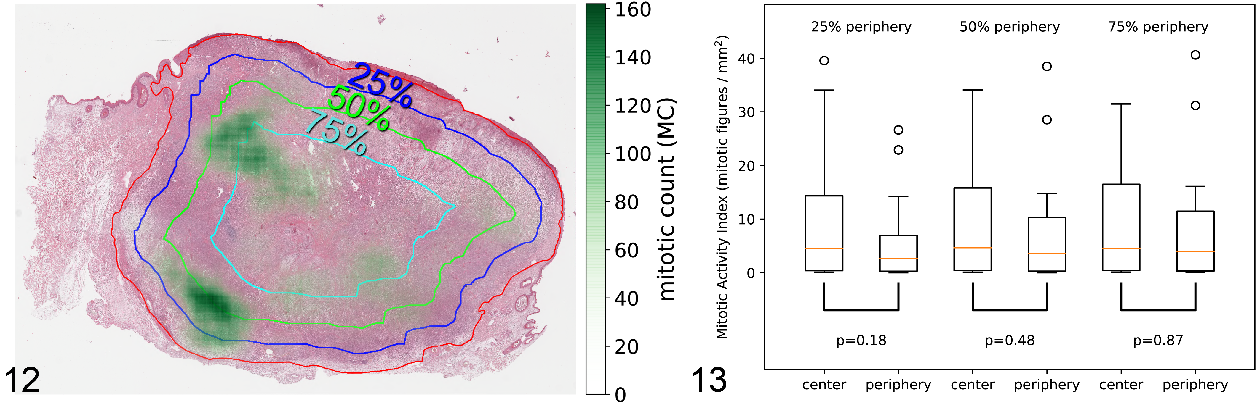
Computerized analysis was used to assess whether the ground truth mitotic density determined by the MAI (count of mitotic figures within the entire periphery or center area divided by the size of the area) varied between the periphery and center of the tumor area in the included ccMCTs. We defined the tumor periphery at 3 different sizes containing 25%, 50%, or 75% of the entire tumor section area (Fig. 12). For a 25% periphery area ratio, the median MAI was 2.65 mitotic figures/mm² for the periphery and 4.55 mitotic figures/mm² for the center (Fig. 13; for values of individual cases, see Suppl. Table S6). In the case of the 50/50 area split, the median MAI was 3.60 mitotic figures/mm² and 4.68 mitotic figures/mm² for the periphery and center, respectively (Fig. 13; for values of individual cases, see Suppl. Table S7). When the periphery contained 75% of the total valid tumor area, the median MAI was 3.98 mitotic figures/mm² for the periphery and 4.55 mitotic figures/mm² for the center (Fig. 13; for values of individual cases, see Suppl. Table S8). A 2-sided t test did not find a significant difference between the 2 groups for any of the 3 area proportions (P = .18, P = .48, and P = .87, respectively). Results were similar between the 3 tumor groups.

Figures 12–13. Comparison of the mitotic density between the tumor periphery and tumor center in 28 canine cutaneous mast cell tumors. Figure 12. Example of the 3 different definitions of the border between the tumor periphery and center in which the mitotic density was determined. Whole-slide image (hematoxylin and eosin) of case No. 22 (mostly high mitotic count) with the manually annotated tumor margins (red line). The blue line indicates the border circumscribing the periphery containing 25% and the center containing 75% of the total tumor area. The green line separates the tumor area in half. The cyan line marks the border between the 75% periphery area and the remaining 25% center area. The green overlay superimposed on the whole-slide image indicates the mitotic count distribution with higher opacities representing higher mitotic counts (scale on the right side). Figure 13. Box-and-whisker plots (0%–100% interval) of the mitotic density of the tumor center and periphery for all cases combined with 3 different size definitions. Mitotic density was determined by the mitotic activity index, which was defined as the number of mitotic figures in a specific tumor area (ie, tumor periphery and center) divided by the size of that area. Two-sided t tests did not show significant differences between the 2 tumor areas for any of the 3 size definitions.

Discussion

To standardize histopathological prognostication, several grading systems have been developed in veterinary pathology, all of which use the MC as one relevant parameter. An example is the 2-tier grading system for ccMCT developed by Kiupel et al.²⁰ This grading system uses the MC as 1 of 4 criteria to differentiate between aggressive high-grade and less aggressive low-grade MCT. Although the use of the MC, which is a seemingly objective absolute number, has increased the reproducibility of tumor grading systems, interobserver inconsistency of the MC can potentially lead to variable prognostication. As the present study has shown, there is a lack of universally valid criteria for selecting the appropriate area to perform the MC. This has possibly led to inconsistency in prior studies and in routine case interpretation. In the present study, we determined that the MC varies throughout ccMCT sections, which can potentially be explained by tumor heterogeneity. The MC varied among different regions of the tumor for those cases that had a high overall range of MCs (absolute variation). However, the relative regional MC variation was even higher for those cases with a small overall range of MCs, although the absolute difference was small and likely of less clinical significance. This paradox needs to be considered when comparing agreement level (such as by the intraclass correlation coefficient), and this is why we decided to omit values for groups 1 and 2. Regardless of the high variability of the MC throughout the study, we found that prognostication of all 28 cases solely based on manual MCs by pathologists was very consistent when a cutoff of 7 was applied.^15,20 High κ values for grading indicated that all participating pathologists were able to perform in consensus with other pathologists (ie, MCs were reproducible among the 11 board-certified pathologists). Only in a small subset of 4 borderline cases with very few ground truth areas having MC ≥7 did the manual MCs commonly not reach the cutoff values (ie, false negative; these tumors were often incorrectly identified as having MC <7 based on manual counts by pathologists). Most manual MCs performed in the cases belonging to group 1, subgroup 2 of group 2, and group 3 were consistently below or respectively above the cutoff value in agreement with the ground truth. Future studies are required to determine whether those “false negatives” are truly low- or high-grade tumors. Borderline cases (group 2) were problematic and might potentially represent those cases in which histopathological prognostication does not fit to the clinical outcome.

The manual MC values of all pathologists had high variation, consistent with counts derived from low to high mitotically active areas of the ground truth MC distribution. However, this high variability rarely affected the prognostication based on current cutoff values. The upper quartile of the MC distribution (ie, the MC in the mitotically most active tumor regions) was reached in only half of the cases; that is, pathologists’ manual counts tended to underestimate the highest MC based on the ground truth data. For group 3 with the highest range of MCs, this was only true for one-third of the manual MCs with a 95% confidence interval that still included 25% (random chance). In addition, agreement of the 11 pathologists on the highest manual MCs was smaller for this group (group 3) in comparison to the overall agreement. Both findings indicate the difficulty in accurately and reproducibly performing the MC in cases with a high range of MCs and a potential large size of the histologic section.

Results of the present study prove that manual MCs often do not represent the most mitotically active tumor regions and suggest that area selection likely has a significant influence on the MC. In addition, the high degree of variability of the MC could also be affected by the degree of interobserver variation in identifying mitotic figures. Such variation has been estimated to range from 6.9% to 54.5% by previous studies, while the present study had a disagreement of 17%.^23,27,44 Regardless, our study demonstrated that accurate and reproducible quantification of the most mitotically active region is hampered by marked interobserver variation in digital slides.

A limitation of the present study is that disease-free intervals and survival times were not available. Therefore, the direct influence of variable area selection and MCs on tumor prognosis could not be determined. However, it is the current scientific consensus that the most mitotically active region (and not the region with mean mitotic activity) correlates best with prognosis.²⁶ Due to the moderate sensitivity of the current method in finding the most mitotically active area, the extent of correlation of the MC with disease outcome may have potentially been underestimated in previous studies. Further studies with large case numbers are required to verify whether the highest MC correlates best with clinical outcome.

There is currently no appropriate recommendation to reliably find the mitotically most active region in ccMCTs. It has been proposed that the periphery of a tumor might be the mitotically more active region due to the location of the most aggressive tumor cells at the invasive front of the tumor.^25,26 However, the present study found a minor but statistically insignificant tendency toward a higher MC in the tumor center for all cases combined. However, individual cases were highly variable in whether the periphery or center of the tumor had higher MCs. These findings imply that the approach to count mitotic figures primarily in the tumor periphery would not improve standardization of the MC in ccMCTs. Larger studies are essential to further evaluate whether the invasive front or the center of the tumor is a more reliable area than the periphery to determine the highest MC. It has also been reported that the MC should be counted in the most cellular regions to standardize the MC.^6,13,25,46 In the present study, we included 3 cases with variable cellular density, and in 1 case, the mitotically most active region was in an area of low cellularity. Although it seems conceivable that areas with lower cellularity may generally have a lower mitotic count, this may not be true for every case and sometimes would have led to underestimation of the MC. Also, all current grading systems in veterinary pathology pay little attention to cellular density in terms of how the MC (a parameter independent of cellular density) is determined. In human breast cancer grading, a volume-corrected MC (MC divided by the estimated proportion of the hpf covered by tumor tissue) has been proposed;¹² however, we speculate that proportion estimates are more difficult in round cell tumors with solitary tumor cells and often minimal tumor stroma. The number of mitotically active cancer cells can also be determined as the mitotic index (MI), which is the number of neoplastic cells with mitotic figures divided by the total number of neoplastic cells within a defined area.²⁵ Although this parameter has been shown to be more reproducible than the mitotic count in some canine and feline tumors,³⁷ it would be too laborious in a diagnostic setting to count all neoplastic cells in a 10-hpf area (in the authors’ experience, there are often between 7000 and 13 000 neoplastic cells in 10 hpf in a ccMCT). Future research will show if the MI can be implemented for routine diagnosis by the aid of computerized image analysis.

Selecting “crucial areas” in borderline cases seems very difficult. As discussed above, scanning the whole-slide image for the area with the highest mitotic density is quite ineffective, especially in cases with a large range of MCs. One would assume that larger tumor sections may have a higher variability of the MC than smaller tumor sections simply based on the likelihood of such variations occurring more commonly in larger samples. In the present study, all tumor sections with a tumor diameter above 16 mm included areas with MC ≥7. Although MCTs with low MC in all regions (group 1) had a maximum largest tumor diameter of 16 mm, borderline MCTs (group 2) and MCTs in which most regions had high MCs (group 3) had maximum tumor diameters as small as 9 mm and 7 mm, respectively. Therefore, tumor diameters were independent of MC at least in some cases and probably are inaccurate for use as a solitary distinguishing feature. In some feline and canine neoplasms (feline cutaneous MCT,³³ feline and canine mammary carcinoma,^29,31 and canine melanocytic neoplasia⁴²), tumor size has indeed been determined to be a prognostic indicator. To the authors’ knowledge, similar systematic investigations have not been performed for canine cutaneous MCTs.

Depending on the cutoff value used for tumor grading, the overall chance to assign a high grade based on the MC alone differed considerably in borderline cases. The 3 cutoff values applied (7, 5, and 10) have been used either as part of grading systems or as solitary prognostic parameters for ccMCT in previous studies.^11,15,20,32 In contrast to previous grading approaches for ccMCT,^11,30 the current grading system developed by Kiupel et al²⁰ comprises only 2 grades.³⁰ In the authors’ experience, some pathologists are more comfortable using a 3-tier system that includes an intermediate grade regardless of the high prognostic and therapeutic uncertainty of the intermediate grade.³⁵ However, as we define biological behavior by the presence or absence of invasion and metastatic spread, an intermediate grade has not yet been proven to give additional prognostic or therapeutic information in ccMCT.^20,35 Borderline cases of the present study should not be classified as an intermediate grade but rather as difficult cases that are prone to inconsistent MC determination around the cutoff value. There are always borderline cases between 2 distinct grades regardless of the number of different cutoffs applied. In fact, a 3-tiered system has borderline cases between the first and second grades as well as between the second and third grades, which might add further variability in grading in comparison to a 2-tiered system. The current results highlight the need to very carefully select the MC cutoff values when establishing a grading system as selection will have a great impact on borderline cases. In addition, it is likely that the MC cutoff value will have to be reevaluated with the development of methods that have higher sensitivity to find the most mitotically active region.

A limitation of this study is that there is some interobserver variation in histologically identifying individual mitotic figures. We tried to reduce this as much as possible for the ground truth data set by blinded labeling of 2 independent pathologists. While the interobserver variability (17%) was relatively small in comparison to previous studies (27%–37%), the variability is based only on 2 pathologists establishing the baseline data.^23,27,48 The morphology of mitotic figures is defined as containing condensed chromosomes with hairy extension while lacking a nuclear membrane.^26,46 However, there are considerable differences in the morphology of mitotic figures depending on the phase of division as well as atypical morphologies and, therefore, discordance seems to be unavoidable to a certain degree. Even for well-trained pathologists, it is difficult to differentiate mitotic figures from some apoptotic and pyknotic cells or overstained nuclei.^23,27,44 In the present study, mitotic figures were annotated in the entire tissue section; however, large areas with necrosis were excluded in a second step. We also excluded labels that were not in concordance by 2 pathologists as it has been recommended to only count unambiguous mitotic figures.²⁵

The examination of whole-slide images scanned at a single focal plane may make it more difficult to identify mitotic figures because of the lack of fine focus and the limited image resolution.⁸ Although scanning at multiple focal planes (z-scanning) is technically available and allows the whole-slide image to be viewed at different levels comparable to the fine focus of light microscopy, it is currently not used for routine diagnosis due to the extended scanning time and the huge file size of the whole-slide image.⁸ To reduce misidentification of mitotic figures, we also excluded all slides with inappropriate image quality, as mitotic figures are increasingly difficult to distinguish from artifacts such as overstained nuclei and necrosis throughout the entire slide.⁶ Last, the specific tumor type (ie, MCTs) may pose an additional challenge for identifying mitotic figures, as large numbers of mast cell granules may mask nuclear details. Limited image resolution and lack of fine focus may have also affected area selection by pathologists for manual MCs as many participants noted additional difficulty in assessing the digital scans for mitoses in comparison to light microscopy.

The present results emphasize the need for further standardization for area selection to achieve higher reproducibility in MC. As discussed above, variations in focal density of mitotic figures throughout the tumor section may pose a severe problem for area selection and subsequently for accurate counting. Improvement options include repeated counts by the same or different pathologists with the purpose of uniformity or to choose the highest count.^13,25,26,29 Regardless of the increased time required, even various repeats would have only slightly increased the chance to find very rare events in the present cases. Alternatively, it has been proposed to increase the size of the area enumerated (eg, to 20 hpf),^10,27 which would also increase time investment and therefore would be rather problematic in a diagnostic setting. Although the latter approach has been suspected to improve reproducibility of the MC by a computer model of human breast cancer,¹⁰ it would also change the MC toward the median value as demonstrated by the current study and, therefore, is inadequate to quantify the most mitotically active region. A new approach for standardization of the MC could be automated image analysis based on deep learning methods. Computerized analysis of a whole-slide image has the potential to reduce laborious tasks while minimizing interobserver variability and maximizing reproducibility.⁸ Several robust deep learning–based algorithms have been developed to detect mitotic figures automatically in human breast cancer tissue,^23,48,49 and similar systems are being investigated for ccMCT.^3,4 However, fully automated mitotic activity estimations still have limitations for clinical applications as current algorithms do not have a high enough sensitivity and specificity (F1 score: 0.66–0.89).^5,21 Therefore, algorithms are not necessarily better at identifying individual mitotic figures in comparison to pathologists; however, they may improve histopathological quantification of mitotic figures by investigating every pixel within the whole-slide images and therefore reduce area-selection bias. Subsequently, a potential way to standardize MCs by computerization is a fully automated preselection of the 10-hpf area with the highest mitotic activity within the entire tumor section (field of interest), as has been shown recently.^3,4 Future research has to determine to which degree a computer-assisted diagnosis system could support the pathologist’s task in tumor grading in a diagnostic situation. As the present study proposes that poor reproducibility of the MC can be explained to some degree by inconsistent area selection, we propose that determining the MC could significantly benefit from further attempts to standardize area selection. Nevertheless, we acknowledge that representative MCs with high prognostic value are furthermore dependent on many other factors such as rapid tissue fixation.⁶ It is also emphasized that further markers of cell proliferation (such as AgNOR and Ki-67) have excellent prognostic value and should be considered supplemental methods for prognostication, especially in borderline cases.⁴⁰

In conclusion, the present study showed that in ccMCTs, the MC may vary tremendously between different tumor areas. Pathologists were often unable to determine the area of the highest MC in whole-slide images, which is especially true for MCTs that had a high range of MCs throughout the tumor. Regardless, detection rate for current cutoff values of manual MCs was generally very reproducible between all pathologists. Inaccuracies in determining the highest MC was problematic only for prognostication in a subset of ccMCTs that contained few areas with ground truth MCs above the cutoff value. Our findings highlight the need for further standardization when quantifying mitotic figures in scanned slides of ccMCT. Computer-assisted diagnosis systems using automated image analyses and deep learning approaches might be a promising solution to accurately and reproducibly identify the area with the highest mitotic activity within large tumor sections.

Supplemental Material

Combined_supplemental_materials-Bertram_et_al_2 - Computerized Calculation of Mitotic Count Distribution in Canine Cutaneous Mast Cell Tumor Sections: Mitotic Count Is Area Dependent

Combined_supplemental_materials-Bertram_et_al_2 for Computerized Calculation of Mitotic Count Distribution in Canine Cutaneous Mast Cell Tumor Sections: Mitotic Count Is Area Dependent by Christof A. Bertram, Marc Aubreville, Corinne Gurtner, Alexander Bartel, Sarah M. Corner, Martina Dettwiler, Olivia Kershaw, Erica L. Noland, Anja Schmidt, Dodd G. Sledge, Rebecca C. Smedley, Tuddow Thaiwong, Matti Kiupel, Andreas Maier and Robert Klopfleisch in Veterinary Pathology

Footnotes

Notes

Author Note

Christof A. Bertram and Marc Aubreville contributed equally to the study.

Declaration of Conflicting Interests

The author(s) declared no potential conflicts of interest with respect to the research, authorship, and/or publication of this article.

Funding

The author(s) received no financial support for the research, authorship, and/or publication of this article.

ORCID iD

Christof A. Bertram

Alexander Bartel

Martina Dettwiler

Matti Kiupel

Robert Klopfleisch

Supplemental Material

Supplemental material for this article is available online.

References

Al-Janabi

van Slooten

H-J

Visser

, et al. Evaluation of mitotic activity index in breast cancer using whole slide digital images. PLoS One. 2013;8:e82576.

Aubreville

Bertram

Klopfleisch

, et al. Slide runner. In: Maier

Deserno

Handels

, et al., eds. Bildverarbeitung für die Medizin 2018. Berlin, Germany: Springer Vieweg; 2018:309–314.

Aubreville

Bertram

Klopfleisch

, et al. Field of interest proposal for augmented mitotic cell count: comparison of two convolutional networks. Paper presented at: Proceedings of the 12th International Joint Conference on Biomedical Engineering Systems and Technologies; February 22-24, 2019; Prague, Czech Republic.

Aubreville

Bertram

Marzahl

, et al. Field of interest prediction for computer-aided mitotic count. arXiv preprint arXiv:190205414. 2019.

Aubreville

Krappmann

Bertram

, et al. A guided spatial transformer network for histology cell differentiation. Paper presented at: Eurographics Workshop on Visual Computing for Biology and Medicine; September 4–6, 2019; Brno, Czech Republic.

Baak

Gudlaugsson

Skaland

, et al. Proliferation is the strongest prognosticator in node-negative breast cancer: significance, error sources, alternatives and comparison with molecular prognostic markers. Breast Cancer Res Treat. 2009;115(2):241–254.

Bertram

Gurtner

Dettwiler

, et al. Validation of digital microscopy compared with light microscopy for the diagnosis of canine cutaneous tumors. Vet Pathol. 2018;55(4):490–500.

Bertram

Klopfleisch

. The pathologist 2.0: an update on digital pathology in veterinary medicine. Vet Pathol. 2017;54(5):756–766.

Boiesen

Bendahl

P-O

Anagnostaki

, et al. Histologic grading in breast cancer: reproducibility between seven pathologic departments. Acta Oncol. 2000;39(1):41–45.

10.

Bonert

Tate

. Mitotic counts in breast cancer should be standardized with a uniform sample area. BioMed Eng OnLine. 2017;16(1):16–28.

11.

Bostock

. The prognosis following surgical removal of mastocytomas in dogs. J Small Anim Pract. 1973;14(1):27–40.

12.

Collan

Kuopio

Baak

, et al. Standardized mitotic counts in breast cancer evaluation of the method. Pathol Res Pract. 1996;192(9):931–941.

13.

Dennis

McSporran

Bacon

, et al. Prognostic factors for cutaneous and subcutaneous soft tissue sarcomas in dogs. Vet Pathol. 2011;48(1):73–84.

14.

Edmondson

Hess

Powers

. Prognostic significance of histologic features in canine renal cell carcinomas: 70 nephrectomies. Vet Pathol. 2015;52(2):260–268.

15.

Elston

Sueiro

Cavalcanti

, et al. Letter to the editor: the importance of the mitotic index as a prognostic factor for survival of canine cutaneous mast cell tumors: a validation study. Vet Pathol. 2009;46(2):362–364.

16.

Gamer

Lemon

Fellows

, et al. Package ‘irr’ Version 0.84.1: Various coefficients of interrater reliability and agreement. 2019. https://cran.r-project.org/web/packages/irr/irr.pdf

17.

Hallgren

. Computing inter-rater reliability for observational data: an overview and tutorial. Tutor Quant Methods Psychol. 2012;8(1):23–34.

18.

Horta

Lavalle

Monteiro

, et al. Assessment of canine mast cell tumor mortality risk based on clinical, histologic, immunohistochemical, and molecular features. Vet Pathol. 2018;55(2):212–223.

19.

Kirpensteijn

Kik

Rutteman

, et al. Prognostic significance of a new histologic grading system for canine osteosarcoma. Vet Pathol. 2002;39(2):240–246.

20.

Kiupel

Webster

Bailey

, et al. Proposal of a 2-tier histologic grading system for canine cutaneous mast cell tumors to more accurately predict biological behavior. Vet Pathol. 2011;48(1):147–155.

21.

Wang

Liu

, et al. DeepMitosis: mitosis detection via deep detection, verification and segmentation networks. Med Image Anal. 2018;45:121–133.

22.

Loukopoulos

Robinson

. Clinicopathological relevance of tumour grading in canine osteosarcoma. J Comp Pathol. 2007;136(1):65–73.

23.

Malon

Brachtel

Cosatto

, et al. Mitotic figure recognition: agreement among pathologists and computerized detector. Anal Cell Pathol. 2012;35(2):97–100.

24.

McSporran

. Histologic grade predicts recurrence for marginally excised canine subcutaneous soft tissue sarcomas. Vet Pathol. 2009;46(5):928–933.

25.

Meuten

Moore

George

. Mitotic count and the field of view area: time to standardize. Vet Pathol. 2016;53(1):7–9.

26.

Meuten

. Appendix: diagnostic schemes and algorithms. In: Meuten

, ed. Tumors in Domestic Animals. New York, NY: John Wiley; 2016:942–978.

27.

Meyer

Alvarez

Milikowski

, et al. Breast carcinoma malignancy grading by Bloom–Richardson system vs proliferation index: reproducibility of grade and advantages of proliferation index. Mod Pathol. 2005;18(8):1067–1078.

28.

Meyer

Cosatto

Graf

. Mitotic index of invasive breast carcinoma: achieving clinically meaningful precision and evaluating tertial cutoffs. Arch Pathol Lab Med. 2009;133(11):1826–1833.

29.

Mills

Musil

Davies

, et al. Prognostic value of histologic grading for feline mammary carcinoma: a retrospective survival analysis. Vet Pathol. 2015;52(2):238–249.

30.

Patnaik

Ehler

MacEwen

. Canine cutaneous mast cell tumor: morphologic grading and survival time in 83 dogs. Vet Pathol. 1984;21(5):469–474.

31.

Peña

Andrés

Clemente

, et al. Prognostic value of histological grading in noninflammatory canine mammary carcinomas in a prospective study with two-year follow-up: relationship with clinical and histological characteristics. Vet Pathol. 2012;50(1):94–105.

32.

Romansik

Reilly

Kass

, et al. Mitotic index is predictive for survival for canine cutaneous mast cell tumors. Vet Pathol. 2007;44(3):335–341.

33.

Sabattini

Bettini

. Grading cutaneous mast cell tumors in cats. Vet Pathol. 2019;56(1):43–49.

34.

Sabattini

Bettini

. Prognostic value of histologic and immunohistochemical features in feline cutaneous mast cell tumors. Vet Pathol. 2010;47(4):643–653.

35.

Sabattini

Scarpa

Berlato

, et al.

Histologic grading of canine mast cell tumor: is 2 better than 3?

Vet Pathol. 2015;52(1):70–73.

36.

Santos

Correia-Gomes

Santos

, et al. Interobserver reproducibility of histological grading of canine simple mammary carcinomas. J Comp Path. 2015;153(1):22–27.

37.

Sarli

Benazzi

Preziosi

, et al. Evaluating mitotic activity in canine and feline solid tumors: standardizing the parameter. Biotech Histochem. 1999;74(2):64–76.

38.

Schott

Tatiersky

Foster

, et al. Histologic grade does not predict outcome in dogs with appendicular osteosarcoma receiving the standard of care. Vet Pathol. 2018;55(2):202–211.

39.

Skaland

van Diest

Janssen

, et al. Prognostic differences of world health organization–assessed mitotic activity index and mitotic impression by quick scanning in invasive ductal breast cancer patients younger than 55 years. Hum Pathol 2008;39(4):584–590.

40.

Sledge

Webster

Kiupel

. Canine cutaneous mast cell tumors: a combined clinical and pathologic approach to diagnosis, prognosis, and treatment selection. Vet J. 2016;215:43–54.

41.

Spangler

Culbertson

Kass

. Primary mesenchymal (nonangiomatous/nonlymphomatous) neoplasms occurring in the canine spleen: anatomic classification, immunohistochemistry, and mitotic activity correlated with patient survival. Vet Pathol. 1994;31(1):37–47.

42.

Spangler

Kass

. The histologic and epidemiologic bases for prognostic considerations in canine melanocytic neoplasia. Vet Pathol. 2006;43(2):136–149.

43.

Thompson

Pearl

Yager

, et al. Canine subcutaneous mast cell tumor: characterization and prognostic indices. Vet Pathol. 2011;48(1):156–168.

44.

Tsuda

Akiyama

Kurosumi

, et al. Evaluation of the interobserver agreement in the number of mitotic figures breast carcinoma as simulation of quality monitoring in the Japan National Surgical Adjuvant Study of Breast Cancer (NSAS-BC) protocol. Jpn J Cancer Res. 2000;91(4):451–457.

45.

Valli

Kass

Myint

, et al. Canine lymphomas: association of classification type, disease stage, tumor subtype, mitotic rate, and treatment with survival. Vet Pathol. 2013;50(5):738–748.

46.

van Diest

Baak

Matze-Cok

, et al. Reproducibility of mitosis counting in 2,469 breast cancer specimens: results from the multicenter morphometric mammary carcinoma project. Human Pathol. 1992;23(6):603–607.

47.

Vascellari

Giantin

Capello

, et al. Expression of Ki67, BCL-2, and COX-2 in canine cutaneous mast cell tumors: association with grading and prognosis. Vet Pathol. 2013;50(1):110–121.

48.

Veta

Van Diest

Jiwa

, et al. Mitosis counting in breast cancer: object-level interobserver agreement and comparison to an automatic method. PLoS One. 2016;11(8):e0161286.

49.

Veta

Van Diest

Willems

, et al. Assessment of algorithms for mitosis detection in breast cancer histopathology images. Med Image Anal. 2015;20(1):237–248.

Supplementary Material

Please find the following supplemental material available below.

For Open Access articles published under a Creative Commons License, all supplemental material carries the same license as the article it is associated with.

For non-Open Access articles published, all supplemental material carries a non-exclusive license, and permission requests for re-use of supplemental material or any part of supplemental material shall be sent directly to the copyright owner as specified in the copyright notice associated with the article.

0.00 MB

108.44 MB