
Abstract
Probability surveys are experiencing important drawbacks nowadays: costs are relatively high and participation rates are decreasing, which could yield less accurate estimates. Alternatively, nonprobability samples like administrative records are having a rise in popularity due to their convenience and low costs. Unfortunately, nonprobability samples are often selective and, as the underlying sampling design is unknown, estimators based on such samples are generally biased. Research is ongoing on how to deal with this selection bias. In this paper, a method is proposed that combines estimators from a probability and nonprobability sample on an aggregated level. Our estimator is constructed as a weighted mean of both estimators. The weight is chosen to minimize the expected value of the mean squared error (MSE) of the combined estimator under an assumed model for the bias in the estimator based on the nonprobability sample. Our method does not require any data on the level of the individual units in the samples. We performed simulation studies where two different methods of modeling the bias in the nonprobability sample were tested. We also applied one of these methods to a real dataset from Statistics Netherlands and showed that the MSE was indeed reduced in a real application.
1. Introduction
The sample survey, and the probability sampling framework with it, emerged as a field in the first half of the twentieth century intending to satisfy the need of keeping a general record of the nationwide population. This need has evolved into more complex ones, increasingly broken down to the point of requiring more and more precise statistics for different subpopulations which we can also call domains. The needs can be reflected by policymakers and by the importance of resource allocation, social program implementation, and environmental planning and by the private market, especially from small businesses that rely on such estimations (Pfeffermann 2002; Rao 2003).
Implementing a probability survey is demanding, but it carries several benefits, the most important being that it allows one to make unbiased inferences about a target population (Lohr 2019). Nevertheless, probability sampling has encountered many drawbacks in the last few years. Due to its high cost, increasing non-response, and debate about the coverage error that this implies, the validity of probability sampling has started to be questioned (Brick 2014).
Alongside that, in the latest years, there has been an increasing interest in the statistical use of data that can be obtained from different data sources far from the probability sampling framework: the so-called nonprobability samples. National Statistical Institutes (NSIs) are particularly interested in nonprobability samples since they are constantly motivated to improve the quality of estimators and reduce data collection costs (Van den Brakel 2019). Examples of nonprobability data at NSIs such as Statistics Netherlands (CBS) are many administrative datasets, such as administrative data from the Tax Office, from energy providers, and from education registers.
A nonprobability sample can be counterproductive for various reasons: there is no clear sampling framework to work with and such data can easily lead to a large bias in estimators because of selectivity. Selectivity is a major issue to deal with when using nonprobability samples. Selectivity refers to the situation in which the part of the target population included in the sample is substantially different from the part of the population that is not included in the sample, making it difficult to make inferences about the target population. Nonprobability samples are likely to be selective regarding the population and the selection probability of units usually remains unknown (M. R. Elliott and Valliant 2017). Nonetheless this type of sample can be considered inexpensive in comparison with a probability one, and methods that try to account for selectivity have been developed. Moreover, the use of nonprobability samples could eventually help reduce the variance of estimators for parameters of interest. In the case of CBS, efforts have been made to go from obtaining estimates from surveys to obtaining them from administrative records, which could be a valuable source of information to overcome the limitations of survey data (Linder et al. 2014).
The increased interest in nonprobability samples can be observed in a large amount of articles on the use of nonprobability samples for estimation purposes in recent years. For example, Baker et al. (2013), M. R. Elliott and Valliant (2017), Cornesse et al. (2020), Valliant (2020), and Rao (2021) provide overviews of methods for dealing with selective nonprobability samples. These papers show that results are not very promising for approaches that rely on nonprobability samples only.
In recent literature various approaches to integrate both probability and nonprobability samples have been proposed. Popular approaches are sample matching (see, e.g., Baker et al. 2013; Rivers 2007; Rivers and Bailey 2009), calibration approaches (see, e.g., Lee 2006; Lee and Valliant 2009), Bayesian approaches (see, e.g., Sakshaug et al. 2019; Wiśniowski et al. 2020), pseudo-weight approaches (see, e.g., M. R. Elliott 2009; M. R. Elliott and Valliant 2017; A.-C. Liu et al. 2023; Valliant and Dever 2011) and doubly robust approaches (see, e.g., Chen et al. 2020; Z. Liu et al. 2023; Yang et al. 2020). Other relevant articles on the use of nonprobability samples for estimation purposes are Meng (2018), who focused on assessing selection error and selection bias in estimators based on nonprobability samples, and Kim and Tam (2021), who examined the situation where a target variable is observed in a probability sample and, with measurement error, also in a nonprobability sample.
In general, the combination of samples has shown more encouraging results than using a nonprobability sample only and that is why the method we investigate in this article combines data from a large nonprobability sample and a small probability sample. Our method can be seen as an extension of an approach proposed by M. N. Elliott and Haviland (2007). Whereas they largely assumed that the bias in the estimator based on the nonprobability sample is known, we relax this assumption by using ideas from Pannekoek and De Waal (1998) to set up a relatively simple model for the bias of this estimator. Based on this model we construct a combined estimator that is a weighted mean of the estimator for the probability sample and the estimator for the nonprobability sample. We restrict attention to categorical data and focus on estimating proportions.
In contrast to most papers on combining probability samples with nonprobability samples, for our proposed method it is not necessary to link the two samples at the level of individual units. It is not even necessary to have any data at the level of individual units: only aggregated data are required. So, our proposed method can be applied in more cases than methods that require data at unit level. Obviously, when data are available at unit level, methods designed for that situation are very likely to give better results than our proposed method, simply because they utilize more information. In the worst case where none of the methods designed for the situation where unit level data for both samples are available gives acceptable results, one can always aggregate those data and apply our proposed method.
The rest of the article is organized as follows. In Section 2, we specify the proposed methodology. In Section 3, we describe the simulation conditions for the assessment of the method and assess its performance. In Section 4 we apply our method to real data from CBS. In Section 5 we summarize our main conclusions and propose suggestions for future research.
2. Methodology
We suppose there is a target population of
Categories per Domain.
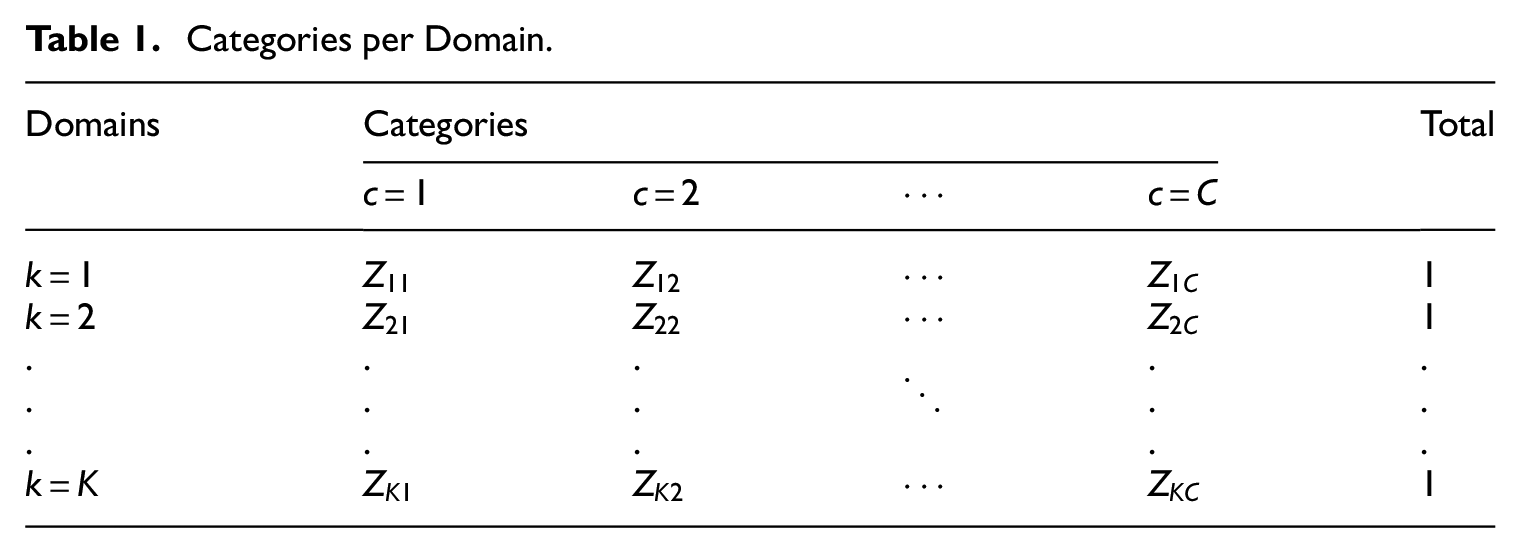
Before we discuss the situation where one of the samples is a probability sample and the other a nonprobability one, we first consider the situation with two independent probability samples
Next, we could construct a combined estimator of the form

where
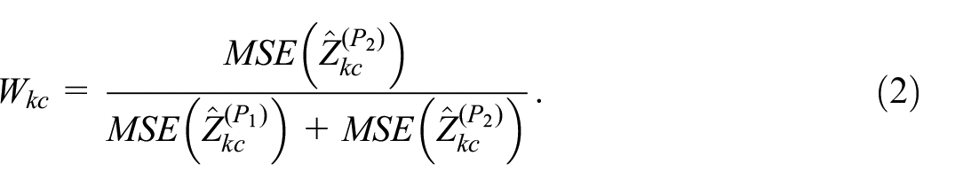
When
In our situation, we have a (small) probability sample
Again, we define a combined estimator

The challenge that we now have in constructing the weight
We define the EMSE of an estimator

where subscript
We can then base the weight in our combined estimator on these EMSEs, analogously to Equation (2):
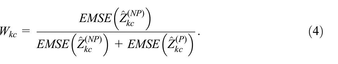
Note that here it is assumed that
We will now derive a weight of the form Equation (4) under a model for the bias
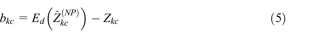
of
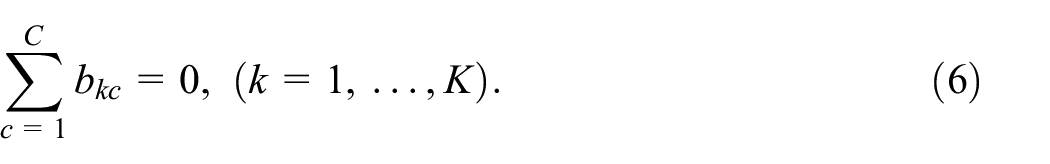
For our basic model, we assume the expected value of the bias is constant across domains but potentially different for different categories. We therefore assume that

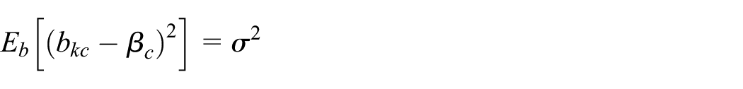
where
Under our model for the bias, we can derive the following expressions for the model-based EMSE of
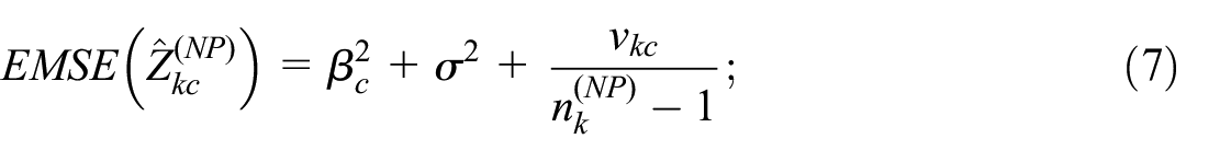
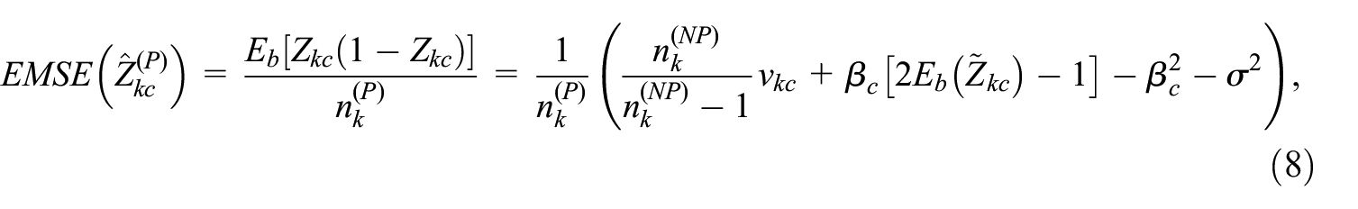
where
Equation (8) may seem surprising, since an obvious estimator for
Substituting the above expressions Equations (7) and (8) into Equation (4) we obtain:
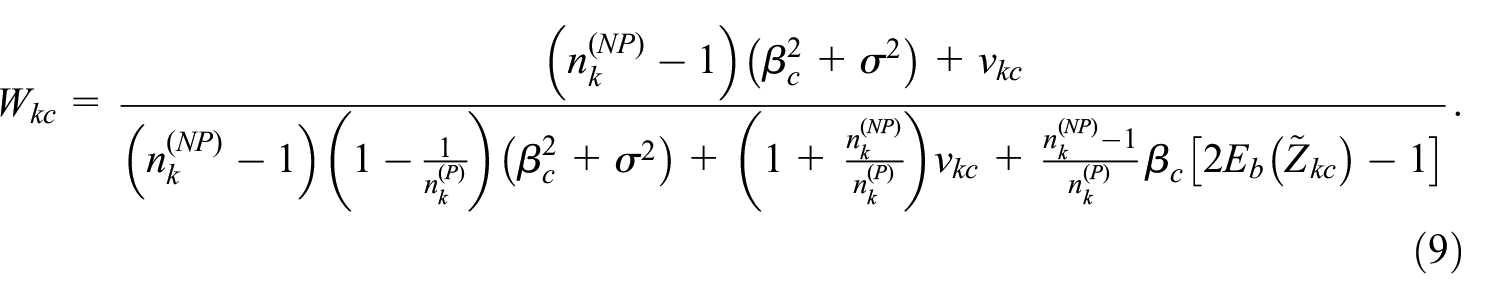
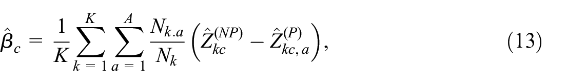
To apply this in practice we need to estimate
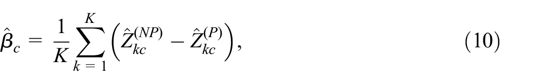
That is, the average difference between the nonprobability and the probability sample for category
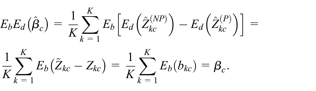
Provided that the number of domains
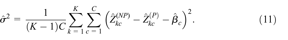
For finite samples this estimator is likely to be biased upwards in practice, since it is also affected by random sampling errors in
By definition unbiased estimators of
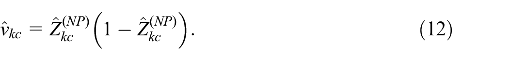
Finally, after calculating
It should be noted that the estimated values
Our approach can be extended by using auxiliary data in various ways. In our simulation study, we focus on a simple extension. For that extension, we assume that an auxiliary variable that partly explains the selectivity of the nonprobability sample is available in the probability sample. An example of such a situation is when the target variable is Educational level (observed in a probability sample and in a nonprobability administrative dataset), the auxiliary variable is Age class (observed in the probability sample), the number of people is known for each combination of Age class and domain, and the inclusion in the administrative dataset on Education level depends on Age class. In such a situation, instead of using Equation (10) to estimate
where
We also examined an even simpler version of our basic model for bias
3. Model Assessment with Simulated Data
3.1. Simulated Conditions
We simulated a population and repeatedly drew a probability sample and a nonprobability one. Then, we estimated the EMSE for
We generated populations consisting of
To generate the data, the units were first assigned randomly to


where
The continuous variable
From the target population, probability samples were drawn with equal inclusion probabilities using SRS, whereas nonprobability samples were drawn with unequal probabilities using randomized systematic sampling, following the approach in Smit (2021), where the probability of inclusion is proportional to
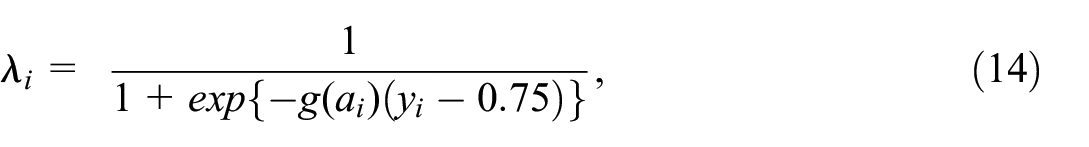
The coefficient
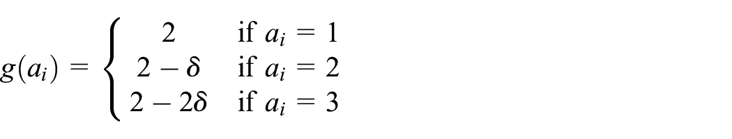
Three different scenarios were considered for the step size
To illustrate the different scenarios, Figure 1 shows the shape of
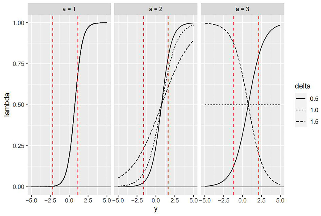
Illustration of
The overall effect of using inclusion probabilities based on Equation (14) was that
Combining all different simulation conditions mentioned above for
3.2. Evaluation
We evaluated the root mean squared error and the bias. First, the root mean squared error was used where
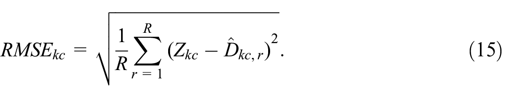
Here
We combined the

Furthermore, we combined the

Instead of using the
Finally, the bias was assessed as the mean of absolute bias (MAB):
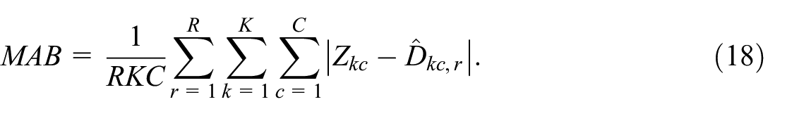
In the next sections we evaluate the performance of our approach in terms of MARMSE and MAB.
3.3. MARMSE and Bias Compared to Single-Sample Estimators
Table 2 presents the percentage of times where the extended combined estimator based on Equation (13) showed a lower MARMSE than the probability sample (PS), the nonprobability sample (NPS), and both samples (Both). Each row in Table 2 varies in number of categories (4 settings), number of domains (4 settings), the size of the probability sample (4 settings), and the size of the nonprobability sample (4 settings), whereas the selectivity and size of categories are kept fixed per row. So, each row summarizes the results over
Proportion (×100%) of Combined Estimators with Lower MARMSE than Single-Sample Estimators.
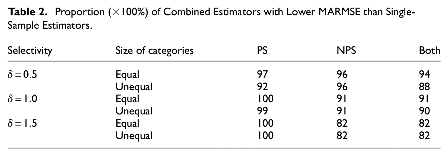
The proportion of times that the combined estimator performed better than an estimator from a nonprobability sample was about 82% in the cases with the weakest selectivity (
The reduction in MARSME that the combined estimator implied in each scenario can be observed in Table 3, which contains the average result of subtracting the MARMSE of the probability sample from that of the combined estimator in column 3, and from subtracting the MARMSE of the nonprobability sample in column 4.
Average Difference Between MARMSE of the Combined Estimator (C) and the Direct Estimators for the Probability (PS) and Nonprobability (NPS) Samples.
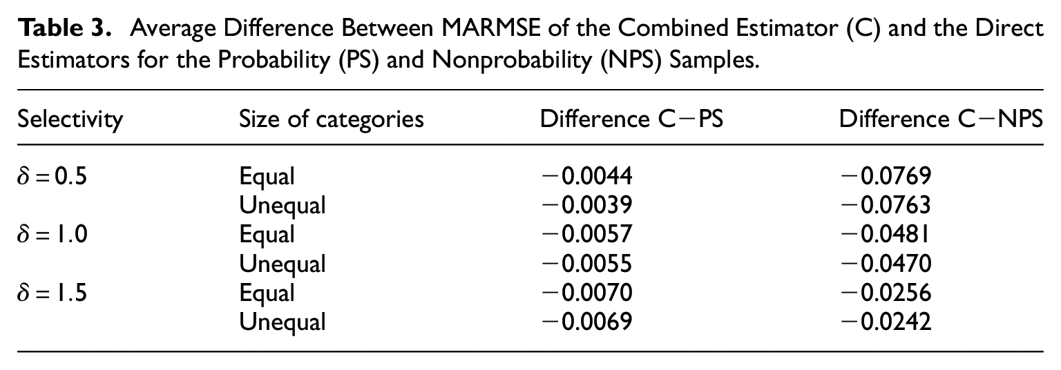
We observe that the average reduction of MARMSE by using the combined estimator was an order of magnitude larger for the nonprobability sample than for the probability sample. For decreasing levels of selectivity (going from
Table B.1 in Appendix B displays the MARMSE for our approach for all conditions with equal-size categories and the strongest selectivity (
For the scenarios with
For larger probability sample sizes than 20, the combined estimator nearly always improved on both estimators when
Tables B.2 and B.3 in Appendix B show similar results for all conditions with equal-size categories and
We have also constructed analogous MARMSE tables for the conditions with unequal category sizes. The patterns in these tables were very similar and did not lead to new insights or different conclusions.
Finally, in terms of bias the results of the simulation study were clear-cut: the combined estimator had a smaller MAB than the estimator based on the non-probability sample in 100% of the conditions examined here.
3.4. Performance of the Combined Estimator Related to the Average Weight
An interesting question for applications is whether situations in which the combined estimator is likely to outperform both individual estimators could be recognized in practice from the available data. A first sight it may seem natural to use the EMSEs of the proposed estimators as indicators for their quality. We can indeed use the EMSEs for this purpose, but only to compare estimators under the same model. We cannot use the EMSEs to compare the performance of estimators computed under different models. In order to compare the performance of estimators computed under different models we need an indicator that is more directly related to the computed estimates.
From the MARMSE results in this simulation study, we have found some evidence that the average value of the weight of the probability sample,
Figure 2 below shows a scatter plot of the simulation results for all scenarios. The horizontal axis shows the average weight
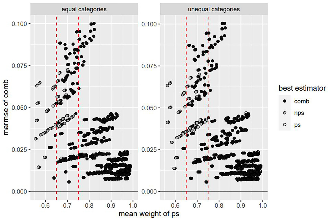
Relation between weight and MARMSE of combined estimator.
In Figure 2, the following pattern is seen. When
3.5. MARMSE and Bias Compared to Other Combined Estimators
Finally, we compared the proposed combined estimator to two other estimators that combine information from the two samples using only aggregated data: the estimator from M. N. Elliott and Haviland (2007; EH) and an estimator based on iterative proportional fitting (IPF).
The EH estimator is also based on Equation (3). Although M. N. Elliott and Haviland (2007) largely assumed that the bias of the estimator based on the nonprobability sample is known, they did suggest a simple estimator for this bias, namely
In the IPF approach we construct a two-dimensional table where the initial internal values are given by
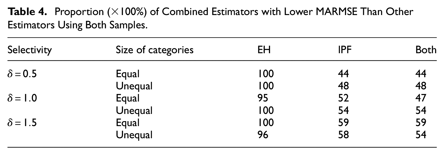
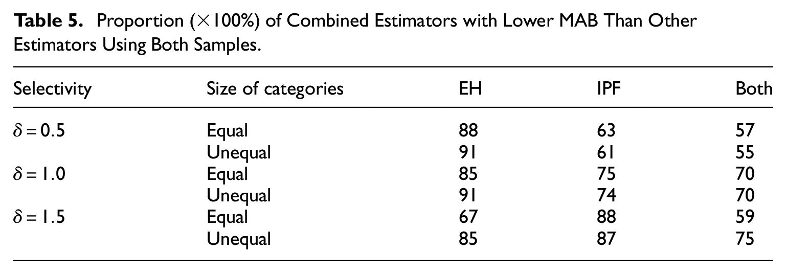
Tables 4 and 5 show the proportion of times that the proposed combined estimator outperformed one or both of these alternative estimators in terms of MARMSE (Table 4) and MAB (Table 5), in a similar format to Table 2. It is seen that the combined estimator nearly always had a smaller MARMSE and usually had a smaller MAB than the EH estimator. The combined estimator also outperformed the IPF estimator in terms of bias most of the time, in particular when the level of selectivity of the nonprobability sample became smaller (rising from
Proportion (×100%) of Combined Estimators with Lower MARMSE Than Other Estimators Using Both Samples.
Proportion (×100%) of Combined Estimators with Lower MAB Than Other Estimators Using Both Samples.
4. Application to Real Data
4.1. Data
The Educational Attainment File (EAF) provided by CBS combines data from the Labour Force Survey and various administrative data sources on the educational level of people. Here, we consider the EAF of the year 2019. The target population consists of all the people who were registered in the Municipal Personal Records Database (the official population register of the Netherlands) on the 1st of October 2019.
The Labour Force Survey (LFS) is a rotating panel survey with five waves, with a target population of people fifteen years or older who live in the Netherlands. The EAF contains LFS data from several years, which have been integrated with other available information from administrative data sources (Linder et al. 2014).
The administrative data sources are nonprobability samples including the following: files with educational histories as submitted by job seekers at the UWV Work company, Central Register of Registrations in Higher Education, Education number files from secondary education, and Education number files from primary education and special education. These records also compile the measurement of educational attainment and contain 11,092,584 observations (i.e., about 64% of the target population of the EAF). It is known that, for historical reasons, these administrative data are selective with respect to age, migration background, and educational attainment itself (older people, people not born in the Netherlands and people with lower attained education levels are more likely to be missing); see Linder et al. (2014) for a detailed analysis of missing data.
For this study, the administrative records in the EAF are treated as a nonprobability sample and
We selected eleven municipalities of different sizes and used those as our domains. In the Netherlands, Municipality is quite unrelated to Education Level, so we are in a situation that is suitable for our method (see also Subsection 2). After selection of the eleven municipalities, we ended up with 17,193 observations from the probability sample, and 623,114 from the nonprobability sample. Highest-attained level of education has originally eighteen categories of unequal size per domain, which we have recoded into three categories, namely lower (1), middle (2), and higher education (3).
For its regular output based on the EAF, CBS computes estimates by weighting the LFS data to represent the subset of the population that is not covered by the administrative records (Linder et al. 2014). The quality of these regular estimates is considered to be very high (see Kuijvenhoven and Scholtus 2010; Linder et al. 2014). We therefore consider these estimates to be the true values and compare our proposed combined estimator based on Equation (10) to these values.
4.2. Results
The situation at hand concerns a target variable with three categories, eleven domains, and mostly quite large sample sizes per domain. The regular CBS estimates and estimates from the estimators for the probability and nonprobability sample and the combined estimator are given in Table 6. In Table 6n(P) and n(NP) denote the sample sizes of the probability sample, respectively the nonprobability sample. Below the name of each municipality the number of inhabitants in 2019 is given.
Estimates of Educational Attainment per Municipality; All Estimates Presented as Rounded Percentages.
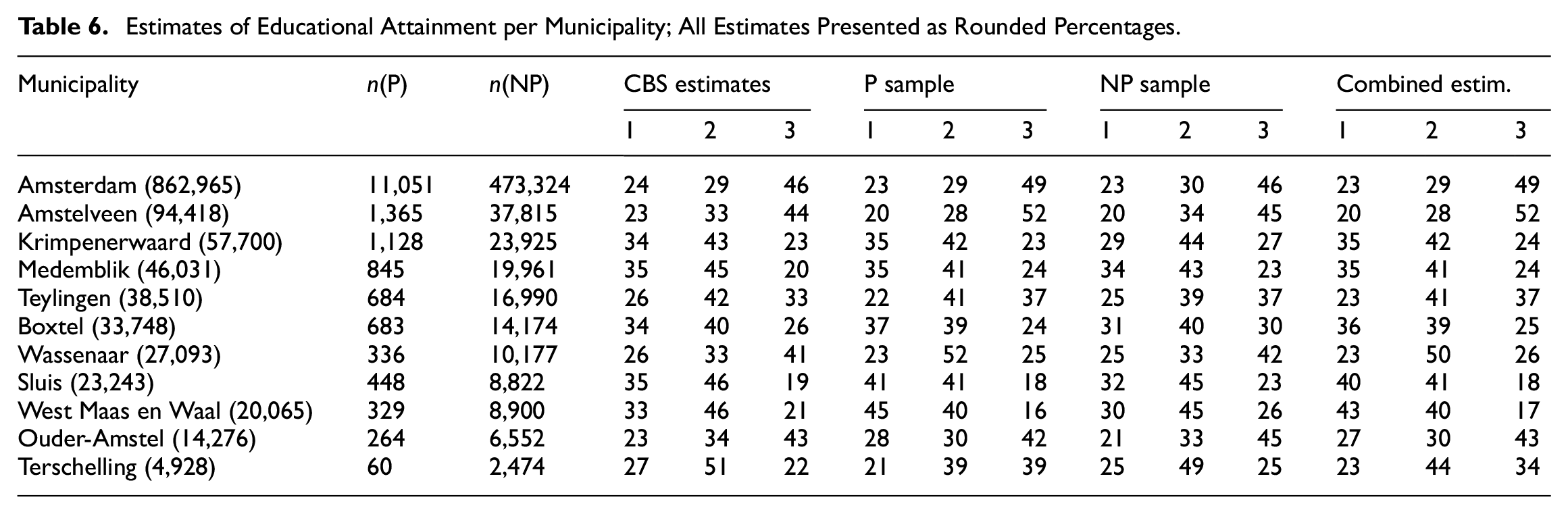
We observe that estimates of the combined estimator are, overall, close to the regular CBS estimates, which we consider the true estimates. Large absolute differences (±10 percentage points or more) are observed in four out of the thirty-three estimates in total. This is the case for categories 2 and 3 in Wassenaar, category 1 in West Maas en Waal, and category 3 in Terschelling. The estimates are not particularly affected by the sample size, since of these three municipalities only Terschelling has a sample size that we would consider small (
The differences between the estimates from the probability sample and the regular CBS estimates can be explained also by three other aspects: first by the different procedures of estimation, second, by differences in the data processing and definitions used, and third, because our target population is from 2019 and we are using a probability sample from 2016, although this still is a reasonable approximation because the distribution of educational attainment changes slowly over the years.
Because these three aspects could have deviated the combined estimator from the estimates from CBS, we have also simulated two scenarios in which we eliminate these three aspects. For the simulation we first draw a new simple random sample with the same sample size (denoted by n(1) in Table 7) as the already mentioned probability sample, and one with a smaller sample size (denoted by n(2) in Table 7), directly from the observed distribution in the EAF. Then, we calculate the combined estimator again with each of the new samples as we can see in Table 7 with their respective sample sizes. For the numbers of inhabitants per municipality in 2019, see Table 6.
Combined Estimator with Simulated Probability Samples of Educational Attainment per Municipality; All Estimates Presented as Rounded Percentages.
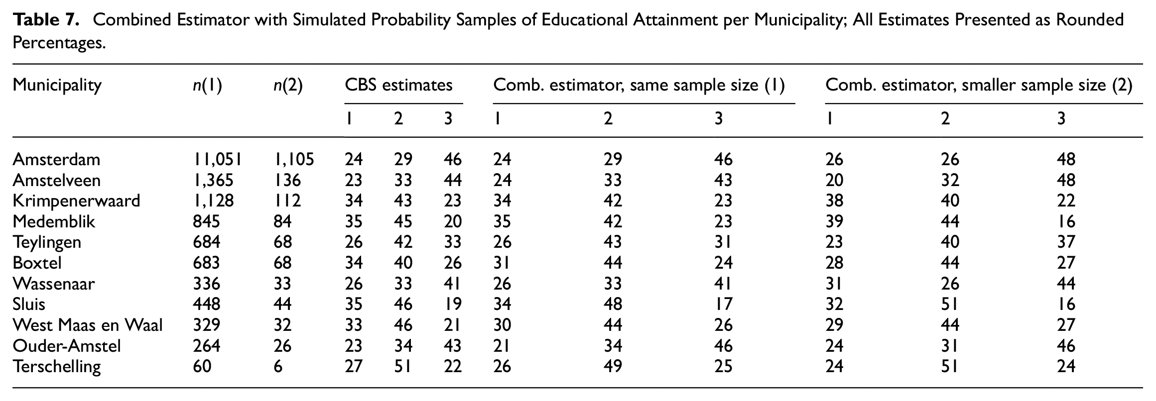
In Table 7 we observe that the difference between the regular estimates from CBS with the ones from the combined estimator computed with a probability sample of the same size as in Table 6 is drastically reduced, with no absolute difference larger than 5 percentage points. Even for a smaller sample size n(2), reduced to a tenth of the original size n(1), estimators are still very close: the largest absolute difference is now 7 percentage points, and only three estimates have an absolute difference larger than 5 percentage points.
5. Discussion
In this study, we have proposed and evaluated a way to combine a probability and a nonprobability sample with the aim of reducing the mean squared error of an estimator of proportions. We proposed a model to estimate the bias of the direct estimator for a nonprobability sample and combine this estimator with the direct estimator for a probability sample, aiming to obtain a combined estimator with a smaller mean squared error.
Through simulation studies, we have shown that the combined estimator can lead to a reduction of the MSE, which we evaluated through the MARMSE of each simulated scenario. This evaluation indicates that using our model for bias
These findings are supported by an empirical application to a real dataset on educational attainment and a simulation based on that dataset using regular CBS estimates as the true values. Here, we have shown that the combined estimator can obtain close estimates to those obtained with methods that have been tested and validated previously and are currently in use.
As already mentioned in the Introduction, our proposed method has the advantage that only aggregated data are required. Furthermore, our method is robust in the sense that it will never yield a worse result, that is, higher MSE, than the highest MSE that was obtained from one of the two samples separately. Finally, the proposed method is very easy to implement in software like R since it requires very few lines of code.
We see various possibilities for extending our method to a wider range of situations. First, in this article we examined a simple way to include available auxiliary data in the estimation procedure, namely by estimating
Second, in this article, we proposed approaches for categorical variables. These approaches could be extended to other types of variables, particularly if they are intended to be used beyond the field of official statistics. For instance, if several continuous variables are of interest and one wants to publish their totals or means per domain, this would require a different model to address the bias in the nonprobability sample.
Third, one important assumption was that we considered the probability sample to be unbiased. We assumed so during this study, but the same problems that probability samples have been facing lately that are already pointed out in the Introduction could mean that this assumption might not be true. The proposed approaches would need to be adapted if this assumption does not hold.
Fourth, for simplicity we developed the combined estimator for an elementary setup, where the probability sample is a simple random sample stratified by domain. In a broader context,
Fifth, in this article we have assumed that
Finally, if one has data at the unit level available, one could in some situations consider using a method designed for that situation to remove part of the selectivity in the nonprobability sample, and then apply our proposed approach on aggregated estimates from the nonprobability sample and a probability sample to mitigate the remaining selectivity.
Footnotes
Appendix A
Appendix B
Acknowledgements
The authors thank a guest editor and three referees for their valuable comments.
Funding
The author(s) received no financial support for the research, authorship, and/or publication of this article.
Data Availability Statement
The research repository of this study can be found in the following GitHub repository: ![]() . The data from Subsection 4 are available in a secure environment at CBS. To get access to the data one needs to contact CBS. The used software was R version 4.2.3 (Subsection 3) and R version 4.1.3 (Subsection 4).
. The data from Subsection 4 are available in a secure environment at CBS. To get access to the data one needs to contact CBS. The used software was R version 4.2.3 (Subsection 3) and R version 4.1.3 (Subsection 4).
Received: June 2023
Accepted: September 2024