Combining Administrative and Survey Data to Correct Coverage Errors in Register-Based Statistics: A Bayesian Approach

Abstract

The statistical production process of many National Institutes is increasingly exploiting the integration of administrative data and sample surveys. Administrative data are generally affected by errors; among others, under and over-coverage may introduce bias in the statistics produced. In this paper, we propose a method to make inference on the population sizes at different aggregation levels by leveraging administrative data in the presence of coverage errors. We introduce a Bayesian statistical model for integrating nonprobability (register-based) and probability samples. The use of a Bayesian model allows a natural quantification of the uncertainty of estimates through the posterior distribution of the unknown target parameters. Although the framework we discuss is quite general, we will mainly refer to the setting of the Italian Permanent Census. We first assess the model performance using simulated data closely related to the real one; then, we provide results for the real data.

1. Introduction

The use of non-survey data, especially administrative data, is becoming crucial in the statistical production system of National Statistical Institutes (NSIs). The reasons for this widespread use are discussed in Citro (2014): a data production context that leverages multiple sources is the best way to meet the user’s needs and to avoid high rates of non-response in questionnaires. A relevant framework concerning the integration of administrative and survey data is that of building statistical registers. Statistical registers allow NSIs to compute different summaries of the target population, including its size. Computing summary statistics directly from registers is an essential task of the NSIs today; the availability of register-based statistics allows the NSIs to have a sort of backbone for some core variables. Under the principles of standardization and coherence, such sources may be used in the production of all the related statistics of the NSIs. This is the case of North European countries that have produced purely register-based statistics since the 1990s (Statistics Denmark 1995; Statistics Finland 2004; Wallgren and Wallgren 2007).

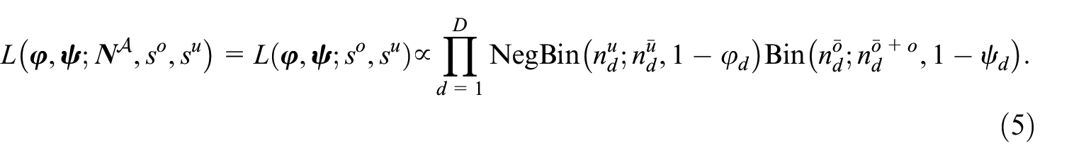
Today, this framework is being adopted in many other countries (Istat 2016), and the register is widely considered a formal and reliable statistical product, where every estimate should be accompanied by its degree of uncertainty. This is a crucial point to consider; in the past, registers were assumed to be affected by negligible errors, while today, they are filtered and processed using old and new statistical methods to account for errors.

Errors may occur in different ways, as discussed by Biemer and Lyberg (2003) and Groves et al. (2011) for sample surveys and by Zhang (2012) for register-based statistics and data integration of nonprobability samples—such as administrative data. For instance, non-probability samples obtained from administrative data sources are typically affected by coverage errors. On the one hand, statistical units belonging to the target population may not be included in the sample (under-coverage); on the other hand, some units that do not belong to the target population may erroneously be included in the sample (over-coverage). For a discussion and illustration of these issues, see Wolter (1986) and Zhang (2015).

In this paper, we propose a Bayesian statistical model to make inference on the population size at different aggregation levels by leveraging administrative data and survey data in the presence of coverage errors. This model naturally accounts for different sources of error and quantifies the uncertainty of the estimates. The flexibility of the Bayesian approach has been proven crucial in managing complex models in similar contexts (see, e.g., the recent Elleouet et al. 2022). Through the simulations and analysis based on the 2018 “Italian Permanent Census” data, we show that a Bayesian approach can manage the different sources of error and adequately summarize the uncertainty through a suitable synthesis provided by the posterior distribution.

The paper is structured as follows: Section 2 describes the general statistical model. Section 3 details the motivating example, namely the 2018 Permanent Census. We empirically assess the model’s performance using a simulated dataset closely reflecting the Permanent Census data in Section 4. In Section 5, the model is applied to real data. The conclusions follow.

2. Model Setting

2.1. Notation

Let $\mathcal{U}$ be a finite population of unknown size $N$ . We denote with $\mathcal{A}$ a non-probability sample of $\mathcal{U}$ , that is, any administrative data source; we assume $\mathcal{A}$ to suffer from under- and over-coverage. Let ${\mathcal{S}}^u$ and ${\mathcal{S}}^o$ be two samples designed to assess the entity of under-coverage and over-coverage errors in $\mathcal{A}$ , respectively. In particular, let ${\mathcal{S}}^u$ be a simple random sample of the target population $\mathcal{U}$ , and let ${\mathcal{S}}^o$ be a simple random sample of the administrative source $\mathcal{A}$ . We aim to estimate the target population size, $N$ , by using $\mathcal{A}$ and leveraging ${\mathcal{S}}^o$ and ${\mathcal{S}}^u$ to correct the coverage errors. Figure 1 schematically shows the overlap of the sources. In the Figure, ${\mathcal{S}}^o$ and ${\mathcal{S}}^u$ do not overlap. We make this mild assumption throughout the paper.

Figure 1.

Representation of the data sources and the target population. The height of the rectangles represents the number of units included in the set; the width represents the amount of information (covariates), which is assumed to be common to all sources. $\mathcal{U}$ is the target population, delimited by the thick solid line. $\mathcal{A}$ , delimited by the dashed line, is the administrative source. $\mathcal{A}$ under-covers $\mathcal{U}$ , and it also includes out-of-target units (over-coverage). ${\mathcal{S}}^o$ (gray rectangle, diagonal lines) is a sample designed to assess the entity of the over-coverage error in $\mathcal{A}$ , and it is typically contained in $\mathcal{A}$ . ${\mathcal{S}}^u$ (gray rectangle, net) is a sample designed to assess the under-coverage error in $\mathcal{A}$ . It is assumed to include units that do and do not belong to $\mathcal{A}$ .

Let $N^{\mathcal{A}}$ be the number of individuals listed in $\mathcal{A}$ . We denote with $N^{\overline{o}}$ the unknown number of units not over-covered by $\mathcal{A}$ , namely the number of units listed in $\mathcal{A}$ that belong to the target population; $|\mathcal{U}\cap \mathcal{A}|=N^{\overline{o}}$ . We also denote with $N^u$ the unknown number of population units missed by $\mathcal{A}$ ; $|\mathcal{U}\setminus \mathcal{A}|=N^u$ . Our goal is to estimate the error-free population size $N=N^{\overline{o}}+N^u$ ; to do so, we leverage the two probability samples ${\mathcal{S}}^o,{\mathcal{S}}^u$ .

Let $n^{\overline{o}+o}$ be the size of ${\mathcal{S}}^o$ (the height of the gray rectangle with diagonal stripes in Figure 1); by design, $n^{\overline{o}+o}\le N^{\mathcal{A}}$ . Among the $n^{\overline{o}+o}$ units, we observe $n^{\overline{o}}$ not over-covered by $\mathcal{A}$ , namely the in target units or units that belong to $\mathcal{U}$ (see again Figure 1); $n^o=n^{\overline{o}+o}-n^{\overline{o}}$ is the observed number of over-covered units.

Similarly, we denote with $n^{\overline{u}+u}=n^{\overline{u}}+n^u$ the number of individuals covered by ${\mathcal{S}}^u$ (the height of the rectangle with the gray net in Figure 1); $n^{\overline{u}}$ are those also covered by $\mathcal{A}$ , whereas $n^u$ is the observed number of those missed by $\mathcal{A}$ . Note that the number of units that are not-over covered by $\mathcal{A}$ and the number of units that are not-under-covered by $\mathcal{A}$ are equal in $\mathcal{A}$ ; in other words, it is the number of in-target units listed in $\mathcal{A}$ . Thus, $n^{\overline{u}}\le N^{\overline{o}}$ .

We leverage the information contained in ${\mathcal{S}}^o$ , ${\mathcal{S}}^u$ to make inference on the probability of being under and over-covered by $\mathcal{A}$ . Then, we will be able to predict $N^{\overline{o}}$ and $N^u$ .

One can be interested in estimating the in-target population at a specific domain level (e.g., municipality, gender, age class). Hence, we add the subscript $d$ , $d=1,\dots ,D$ , to denote the count at a specific domain level, for example, $N_d^{\overline{o}}$ , $N_d^u$ . We denote with bold letters the vectors of counts, for example, $N^{\mathcal{A}}=(N_1^{\mathcal{A}},\dots ,N_D^{\mathcal{A}})$ . Table 1 helps visualize the observed data structure.

Table 1.

Example of Observed Data Structure.

$d$	$N_d^{\mathcal{A}}$	$n_d^{\overline{o}+o}$		$n_d^{\overline{u}+u}$
		$n_d^{\overline{o}}$	$n_d^o$	$n_d^{\overline{u}}$	$n_d^u$
$1$	$N_1^{\mathcal{A}}$	$n_1^{\overline{o}}$	$n_1^o$	$n_1^{\overline{u}}$	$n_1^u$
$2$	$N_2^{\mathcal{A}}$	$n_2^{\overline{o}}$	$n_2^o$	−	−
$3$	$N_3^{\mathcal{A}}$	−	−	$n_3^{\overline{u}}$	$n_3^u$
⋮	⋮	⋮	⋮	⋮	⋮
$D$	$N_D^{\mathcal{A}}$	−	−	−	−

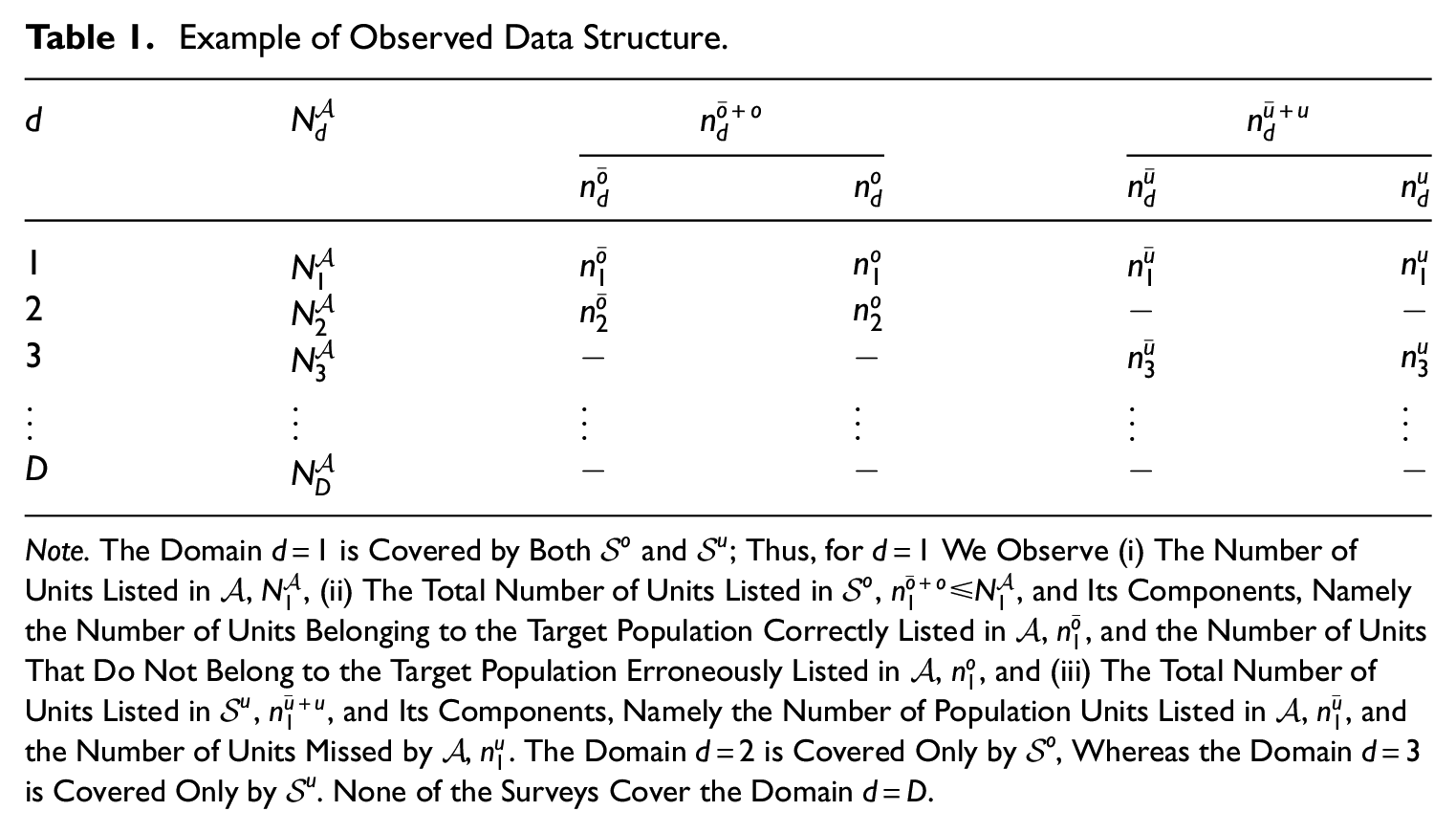
Note. The Domain $d=1$ is Covered by Both ${\mathcal{S}}^o$ and ${\mathcal{S}}^u$ ; Thus, for $d=1$ We Observe (i) The Number of Units Listed in $\mathcal{A}$ , $N_1^{\mathcal{A}}$ , (ii) The Total Number of Units Listed in ${\mathcal{S}}^o$ , $n_1^{\overline{o}+o}\le N_1^{\mathcal{A}}$ , and Its Components, Namely the Number of Units Belonging to the Target Population Correctly Listed in $\mathcal{A}$ , $n_1^{\overline{o}}$ , and the Number of Units That Do Not Belong to the Target Population Erroneously Listed in $\mathcal{A}$ , $n_1^o$ , and (iii) The Total Number of Units Listed in ${\mathcal{S}}^u$ , $n_1^{\overline{u}+u}$ , and Its Components, Namely the Number of Population Units Listed in $\mathcal{A}$ , $n_1^{\overline{u}}$ , and the Number of Units Missed by $\mathcal{A}$ , $n_1^u$ . The Domain $d=2$ is Covered Only by ${\mathcal{S}}^o$ , Whereas the Domain $d=3$ is Covered Only by ${\mathcal{S}}^u$ . None of the Surveys Cover the Domain $d=D$ .

2.2. Bayesian Model for Coverage Errors’ Correction

To predict the population counts at the specified domain level, one needs to learn about the probabilities of under- and over-coverage. In a Bayesian framework, it amounts to say that one must compute the joint posterior distribution of such probabilities, which are considered random. To this aim, we first explicitly state the likelihood function arising from our model and then discuss suitable prior distributions for the unknown parameters of the model.

This section describes a hierarchical Bayesian model for combining information from a non-probabilistic sample (from an administrative source) and the two random samples. In the first stage, we introduce a statistical model for describing the data-generation mechanism and deduce the resulting likelihood function; then, we model the probabilities of under- and over-coverage and specify the prior setting.

We assume that, independently for each domain $d=1,\dots ,D$ , the numbers of not over-covered units, $N_d^{\overline{o}}$ , can be considered as the number of successes that occur in $N_d^{\mathcal{A}}$ independent Bernoulli trials:

$$N_d^{\overline{o}}\mid {\psi }_d~\mathrm{Bin}(N_d^{\mathcal{A}},1-{\psi }_d),d=1,\dots ,D,$$

(1)

where ${\psi }_d$ is the probability of failure, that is, the probability of over-coverage, for domain $d$ ; more explicitly,

$$P(N_d^{\overline{o}}=q;{\psi }_d)=\left(\begin{array}{c}{N}_d^{\mathcal{A}}\hfill \\ \multicolumn{1}{c}{q}\end{array}\right){(1-{\psi }_d)}^q{\psi }_d^{N_d^{\mathcal{A}}-q}d=1,\dots ,D;q=1,\dots ,N_d^A.$$

(2)

Regarding the under-covered counts, we still assume independence among domains. However, assuming a Binomial model is not suitable in this case since we do not have a well-defined number of Bernoulli trials. Yet, one can interpret the number of units missed by $\mathcal{A}$ as the number of failures that occur before $N_d^{\overline{o}}$ successes are observed. Let us denote with ${\phi }_d$ the probability of failure, namely the probability of under-coverage, for domain $d$ ; thus,

$$N_d^u\mid N_d^{\overline{o}},{\phi }_d~\mathrm{NegBin}(N_d^{\overline{o}},1-{\phi }_d)d=1,\dots ,D,$$

(3)

That is,

$$P(N_d^u=r;N_d^{\overline{o}},{\phi }_d)=\left(\begin{array}{c}{N}_d^{\overline{o}}+r-1\hfill \\ \multicolumn{1}{c}{r}\end{array}\right){\phi }_d^r{(1-{\phi }_d)}^{N_d^{\overline{o}}}d=1,\dots ,D;r=0,1,2,\dots$$

(4)

We assume simple random sampling for both ${\mathcal{S}}^o$ and ${\mathcal{S}}^u$ , and independence across domains; under such assumptions, one can combine the modeling assumptions in Equations (3) and (1) and write the likelihood function of the parameters’ vector $(\mathit{\phi }=({\phi }_1,\dots ,{\phi }_D),\mathit{\psi }=({\psi }_1,\dots ,{\psi }_D))$ as

$$L(\mathit{\phi },\mathit{\psi };{\mathit{N}}^{\mathcal{A}},s^o,s^u)=L(\mathit{\phi },\mathit{\psi };s^o,s^u)\propto \underset{d=1}{\overset{D}{\Pi }}\mathrm{NegBin}(n_d^u;n_d^{\overline{u}},1-{\phi }_d)\mathrm{Bin}(n_d^{\overline{o}};n_d^{\overline{o}+o},1-{\psi }_d).$$

(5)

It is important to stress that the hypothesis of simple random sampling for both ${\mathcal{S}}^o$ and ${\mathcal{S}}^u$ allows us to assume that the population model can be reproduced in the observed sample. However, it might happen that, in similar situations, one must consider more complex sample designs; in those cases, calibrating likelihood or Bayesian procedures is generally problematic, and some approximations are often unavoidable. Things are even more complicated in the presence of non-ignorable non-response patterns, which have to be considered in the sampling model; see, for example, Wang et al. (2018) for a discussion of these issues.

In the second stage, we model the probabilities of over and under-coverage as

$$\mathrm{logit}\left({\psi }_d\right)={\mathit{X}}_d\mathbf{\beta }+b_d,d=1,\dots ,D,$$

(6)

and

$$\mathrm{logit}\left({\phi }_d\right)={\mathit{X}}_d\mathbf{\delta }+c_d,d=1,\dots ,D,$$

(7)

where $\mathit{X}$ is the $D\times (1+K^{\text{'}})$ design matrix, with $K^{\text{'}}$ being the number of covariates included in the models, and $b_d$ and $c_d$ are random intercepts;

$$b_d~\mathrm{N}(0,s_b^2),c_d~\mathrm{N}(0,s_c^2),$$

(8)

independently for each $d$ , with $s_b$ and $s_c$ unknown.

The probabilities of under and over-coverage, $\mathit{\phi }$ and $\mathit{\psi }$ , are deterministic transformation of $\mathbf{\beta },\mathit{b}$ and $\mathbf{\delta },\mathit{c}$ , respectively; thus, the unknown parameters of interest are $\mathbf{\beta },\mathbf{\delta },\mathit{b},\mathit{c},s_b^2,s_c^2$ . Since the distributions for $\mathit{b}$ and $\mathit{c}$ are given by the second-level model specification, we only need to specify the joint prior distribution for the remaining unknowns. Hence, let the parameter vector of our model be

$$\mathbf{\theta }=(\mathbf{\beta },\mathbf{\delta },s_b^2,s_c^2).$$

We assume the elements of $\mathbf{\theta }$ to be a priori independent, and we set

$$\begin{array}{c}\mathbf{\beta },\mathbf{\delta }{~}^{\mathrm{iid}}{\mathrm{N}}_{1+K^{\text{'}}}(0,{\omega }^2\mathit{I}),\hfill \\ s_b,s_c{~}^{\mathrm{iid}}\mathrm{Unif}(0,u)\hfill \end{array}$$

(9)

with ${\omega }^2$ and with $u$ known. The values of ω and u can be calibrated by considering that the range of significant values for the coefficients of a logistic regression rarely goes outside the interval (-5,5). However, it is a good practice to test the sensitivity of the results to different prior specifications.

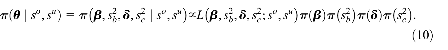
The posterior distribution, which is proportional to the product of the likelihood and the parameters’ joint prior, will be

$$\pi (\mathbf{\theta }\mid s^o,s^u)=\pi (\mathbf{\beta },s_b^2,\mathbf{\delta },s_c^2\mid s^o,s^u)\propto L(\mathbf{\beta },s_b^2,\mathbf{\delta },s_c^2;s^o,s^u)\pi \left(\mathbf{\beta }\right)\pi \left(s_b^2\right)\pi \left(\mathbf{\delta }\right)\pi \left(s_c^2\right).$$

(10)

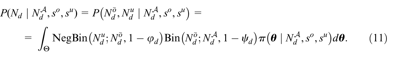
Our goal is the predictive distribution

$$P(N_d\mid N_d^{\mathcal{A}},s^o,s^u)=P(N_d^{\overline{o}},N_d^u\mid N_d^{\mathcal{A}},s^o,s^u)=={\int }_{\Theta }\mathrm{NegBin}(N_d^u;N_d^{\overline{o}},1-{\phi }_d)\mathrm{Bin}(N_d^{\overline{o}};N_d^{\mathcal{A}},1-{\psi }_d)\pi (\mathbf{\theta }\mid N_d^{\mathcal{A}},s^o,s^u)d\mathbf{\theta }.$$

(11)

We obtain a posterior sample via Hamiltonian Monte Carlo algorithm implementing the model in Stan (Stan Development Team 2023).

3. 2018 Italian Permanent Census Data

3.1. The Motivating Example

In 2018, Italy shifted from a survey-based paradigm to a register-based one, establishing the Italian Permanent Population Census (Falorsi 2017). Population counts were produced using an integrated administrative source, the Base Register of Individuals (BRI), corrected for over- and under-coverage by two sample surveys. Righi et al. (2021) proposed, similarly to Pfeffermann et al. (2015), to estimate population counts by correcting the BRI counts with a function of the probabilities of under- and over-coverage estimated on two distinct sample surveys designed to account for coverage errors. The two samples consisted of (i) a list survey, a probabilistic sample of the BRI, and (ii) an area survey, a probabilistic sample of the target population. The list survey was designed to estimate the over-coverage, whereas the area survey was designed to assess the under-coverage. Both surveys used a two-stage sampling design, with the Italian municipalities as the primary sampling units. The secondary sampling units differed in the two samples: the households for the list sample and either addresses or enumeration areas for the area sample. A strategy proposed by Mancini and Toti (2014) consisted of applying a GLMM approach to obtain probabilities of over and under-coverage at an individual level, conditional on individual characteristics such as gender, age, and citizenship. The major limitation of that approach was that the analytical form of the correction term, based on the plugged-in estimated weights, made it very complex to obtain an explicit expression for the accuracy evaluation of the count estimates. The analysis of the Italian municipalities proceeded separately for each Italian Region (NUTS2) and differently for municipalities with a population above or below 18,000 individuals. The aim was to estimate the population counts for each municipality at the profile level, with profiles determined by the combinations of some individual characteristics: individuals’ sex, age class, and citizenship.

Here, we consider the 2018 Permanent Census our motivating example; however, in this work, we make a simplifying assumption and consider the list and area surveys as simple random samples; see Subsection 2.2. We further discuss our simplifying assumption in the Conclusions.

3.2. An Application of the Theoretical Model

We exploit the idea of the Permanent Census to empirically assess the performance of the model introduced in Section 2. The notation introduced in Subsection 2.1 is suitable to the aim; however, instead of considering a generic domain $d$ , we need to consider cells defined by the couple $\{h,q\}$ , with $h$ , $h=1,\dots ,H$ , representing the municipality of residency, and $q$ , $q=1,\dots ,Q$ , denoting the individuals’ profile, determined by the combinations of some individual characteristics.

As covariates in the logistic regressions modeling the over- and under-coverage probabilities (Equations (6) and (7)), we use the whole set of variables that define the profiles $q$ , namely sex, age class, and citizenship, with an additional variable representing to which area, either rural or urban, the municipality belongs to. Hence, $\mathit{X}=({\mathit{X}}^{\mathrm{sex}},{\mathit{X}}^{\mathrm{age}},{\mathit{X}}^{\mathrm{cit}},{\mathit{X}}^{\mathrm{area}})$ where

• $X_{h,q}^{\mathrm{sex}}$ , $h=1,\dots ,H,q=1,\dots ,Q$ , takes value 1 if the individuals composing the count are females and 0 otherwise;

• $X_{h,q}^{\mathrm{age}}$ , $h=1,\dots ,H,q=1,\dots ,Q$ , is a five-level variable indicating the individuals’ age class (0–5; 6–19; 20–39; 40–64; $\ge$ 65); for this variable, we create four dummies, the first class being the reference class;

• $X_{h,q}^{\mathrm{cit}}$ , $h=1,\dots ,H,q=1,\dots ,Q$ , takes value 1 if the individuals have not the Italian citizenship and 0 otherwise;

• $X_{h,q}^{\mathrm{area}}$ , $h=1,\dots ,H,q=1,\dots ,Q$ , takes value 1 if the municipality $h$ is located in an urban area and 0 if it is in a rural area.

The random effects vary according to groups defined by the interactions between the area (as defined above) and the province (NUTS3) to which the municipality belongs. We estimate separate models for the twenty Italian Regions: Abruzzo (ABR), Basilicata (BAS), Calabria (CAL), Campania (CAM), Emilia-Romagna (EMI), Friuli-Venezia Giulia (FRI), Lazio (LAZ), Liguria (LIG), Lombardy (LOM), Marche (MAR), Molise (MOL), Piedmont (PIE), Puglia (PUG), Sardinia (SAR), Sicily (SIC), Trentino-Alto Adige (TRE), Tuscany (TOS), Umbria (UMB), Aosta Valley (VAL), Veneto (VEN).

In the next section, we assess the model’s performance regarding coverage, bias, and variability using simulated data that closely mimic the 2018 Permanent Census. In Section 5, we analyze accurate 2018 Permanent Census data.

4. Simulation Study

To empirically test the model’s performance, we simulate a complete synthetic dataset on which it is possible to distinguish all (otherwise unknown) components of the population: the units correctly listed in $\mathcal{A}$ , those over-covered, and those missed by $\mathcal{A}$ . We restrict our attention to municipalities with a population below 18,000.

In the next subsection, we describe the data simulation; results are shown in Subsection 4.2.

4.1. Data Simulation

First, we generate a synthetic data set composed of three components: (1) units that belong to the target population, $N_{h,q}^{\overline{o}},h=1,\dots ,H,q=1,\dots ,Q$ , and are included in the non-probability sample obtained from the administrative source, (2) units that do not belong to the target population but are included in the non-probability sample (over-coverage component), $N_{h,q}^o,h=1,\dots ,H,q=1,\dots ,Q$ , and (3) units that are in the population but are not included in the non-probability sample (under-coverage components), $N_{h,q}^u,h=1,\dots ,H,q=1,\dots ,Q$ . Then, we draw the under and over-coverage samples from this synthetic data set.

The parameters used to generate this synthetic data set are based on the 2018 Census data. The details of the simulation follow.

• 1. Generation of a data set

We start with a data set composed of real counts of the Base Register of the Individuals involved in the 2018 Italian Permanent Census, $\{N_{h,q}^{\mathcal{A}}\}$ , $h=1,\dots ,H,q=1,\dots ,Q$ . Then, for each municipality $h$ and profile $q$ :

1.1 We randomly generate the count of subjects that are correctly enumerated in $\mathcal{A}$ , $N_{h,q}^{\overline{o}}$ , drawing from a binomial distribution with probability parameter equal to the relative frequency $f_{h,q}^{\overline{o}}$ of not over-covered subjects in ${\mathcal{S}}^o$ :

$$N_{h,q}^{\overline{o}}~\mathrm{Bin}(N_{h,q}^{\mathcal{A}},1-{\psi }_{h,q}\equiv f_{h,q}^{\overline{o}}),h=1,\dots ,H,q=1,\dots ,Q.$$

(12)

1.2 We randomly generate the count of under-covered subjects, $N_{h,q}^u$ , drawing from a negative binomial distribution with the number of successes equal to the number of not under-covered units, and using the relative frequency $f_{h,q}^{\overline{u}}$ of not under-covered subjects in ${\mathcal{S}}^u$ as probability of success:

$$N_{h,q}^u~\mathrm{NegBin}(N_{h,q}^{\overline{o}},1-{\phi }_{h,q}\equiv f_{h,q}^{\overline{u}}),h=1,\dots ,H,q=1,\dots ,Q.$$

(13)

The values ${\mathit{f}}^{\overline{o}},{\mathit{f}}^{\overline{u}}$ are set on the observed relative frequencies of the not over- and not under-covered units in the surveys conducted for the 2018 Italian Permanent Census; yet, we will estimate $\mathit{\psi }$ and $\mathit{\phi }$ assuming two logistic models, as detailed in Subsection 2.2. We denote with $N_{h,q}^{*}$ the (synthetic) target population size for municipality $h$ and profile $q$ , that is, $N_{h,q}^{*}=N_{h,q}^{\overline{o}}+N_{h,q}^u$ .

• 2. Drawing of the two samples for coverage correction

For each municipality, $h,h=1,\dots ,H$ , two simple random samples without replacement representing under and over-coverage samples are drawn from the synthetic data set previously generated. The samples are drawn only considering municipalities used in the actual 2018 sample survey census wave.

4.2. Analysis of the Synthetic Data and Results

The simulation of a synthetic data set, as detailed in the previous subsection, allows us to evaluate the performance of the proposed model knowing the (simulated) target population size, $N_{h,q}^{*},h=1,\dots ,H,q=1,\dots ,Q$ .

Before presenting the simulations’ results, let us naively compare the target population size to that estimated using the administrative source. Let us set $N_h^{\mathcal{A}}=\sum _q{N}_{h,q}^{\mathcal{A}}$ , and, similarly, $N_h^{*}=\sum _q{N}_{h,q}^{*}$ . We define the following measure of relative error of the nonprobability sample derived by the administrative source at the municipal level:

$${\mathrm{RE}}_h^{\mathcal{A}}=\frac{\mid N_h^{\mathcal{A}}-N_h^{*}\mid }{N_h^{\mathcal{A}}}.$$

(14)

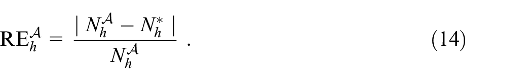
Figure 2 shows distribution of the ${\mathrm{RE}}_h^{\mathcal{A}}$ by Italian Regions (NUTS2). In each region, the relative error for most of the municipalities is below 5%. The region of Marche (MAR) has an outliers’ behavior markedly different from the others, with some municipalities over 10% and reaching a maximum of about 30%.

Figure 2.

Distribution of the municipal ${\mathrm{RE}}_h^{\mathcal{A}}$ (see Equation (14)), by region.

Now, we implement the model described in Section 2 and detailed in Subsection 3.2 with the aim of obtaining population size estimates closer to the target population size than the administrative counts. A Bayesian approach allows us to estimate the posterior distributions of population sizes at the profile level; consequently, any aggregation at the municipal or provincial level is easy to obtain. For instance, Figure 3 shows an example of a single municipality’s posterior distribution of counts. The solid line represents the (simulated) target population size $N_h^{*}$ ; the highest posterior density interval at 95% level (HPD95%, the gray area) covers $N_h^{*}$ . The administrative count for that municipality (dashed line) is far from $N_h^{*}$ . In the following subsections, we investigate the coverage with respect to the simulated target population value, the relative bias of our estimates, and their variability.

Figure 3.

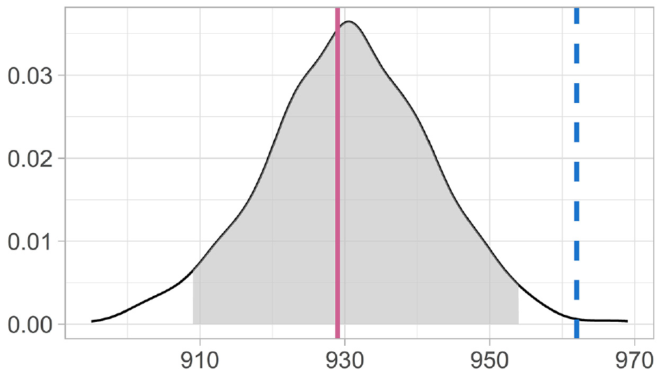
Example of a posterior distribution of counts for a single municipality $h$ . The solid line represents the simulated population value $N_h^{*}$ , whereas the dashed line represents the administrative count $N_h^{\mathcal{A}}$ , clearly affected by a high over-coverage error. The gray shade represents the highest posterior density interval at 95% credibility level (HPD95%).

For this simulation study, we have specified the hyperparameters of our model as follows: ${\omega }^2=25$ , and $s_b,s_d$ uniformly distributed in $(0,10)$ . The results are robust to different prior specifications. Even for the largest regions, less than five minutes are required for the posterior estimation and prediction.

4.2.1. Coverage

The coverage of the proposed method is explored in Figure 4, which is a map showing the coverage by province. Figure 4a shows the coverage at the profile level for each province,

$$\frac{\sum _{h\in \mathrm{pv}}{\mathbb{1}}_{\{N_{h,q}^{*}\in \mathrm{HPD}95\mathrm{\%}\left(N_{h,q}\right)\}}}{\sum _h{\mathbb{1}}_{\{h\in \mathrm{pv}\}}},\mathrm{pv}=1,\dots ,107,$$

(15)

whereas Figure 4b shows the coverage at the municipal level for each province $\mathrm{pv}$ , that is,

$$\frac{\sum _{h\in \mathrm{pv}}{\mathbb{1}}_{\{N_h^{*}\in \mathrm{HPD}95\mathrm{\%}\left(N_h\right)\}}}{\sum _h{\mathbb{1}}_{\{h\in \mathrm{pv}\}}},\mathrm{pv}=1,\dots ,107.$$

(16)

The profile level coverage (Figure 4a) is extensively high, that is, around 95%. There are exceptions. For instance, coverage is below 75% for the provinces of Trieste (TRE), Bologna (EMI), Latina (LAZ), Ragusa, and Siracusa (SIC). Yet, looking at the municipal level coverage (Figure 4b), we can observe a critical improvement. The coverage is still under 75% for the province of Latina (LAZ) only.

Figure 4.

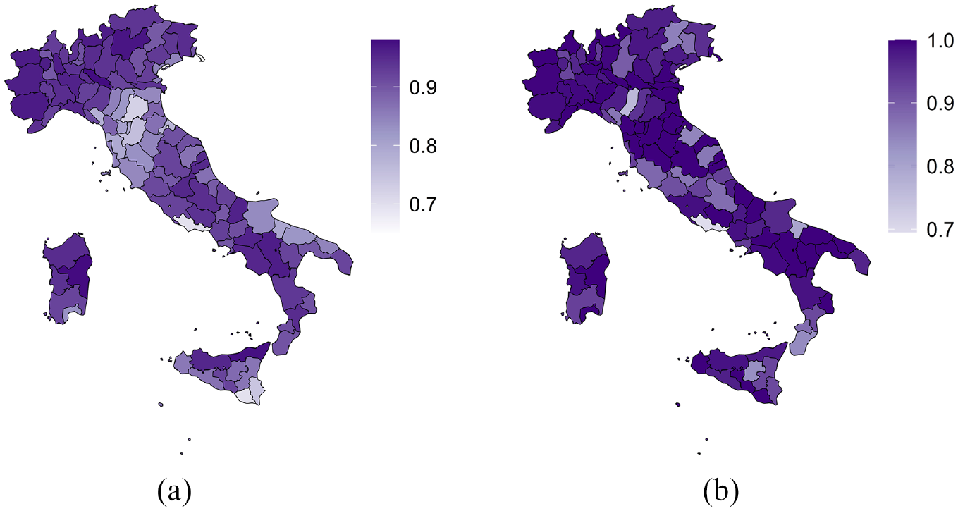
Coverage at the profile and municipal level, HPD95%. Provincial average. Simulated data. (a) Profile level and (b) municipal level.

4.2.2. Relative Bias

Beyond coverage, we may also look at a relative measure of the bias of our estimates, evaluated as:

$${\mathrm{RE}}_h=\frac{\mid \mathrm{Med}\left(N_h\right)-N_h^{*}\mid }{\mathrm{Med}\left(N_h\right)},h=1,\dots ,H,$$

(17)

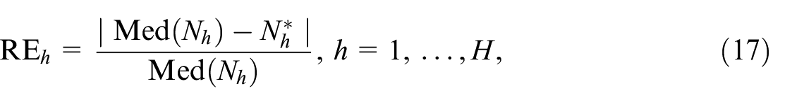
where Med $\left(N_h\right)$ is the posterior median of $N_h$ . Although we do not observe much difference between the posterior median and the posterior mean, we opt for the former for robustness reasons. The RE is analogous to the measure in Equation (14); here, we measure the relative distance of the simulated target population count from the posterior median. To better appreciate the relative gain we obtain via correction in terms of relative error, that is, $({\mathrm{RE}}_h^{\mathcal{A}}-{\mathrm{RE}}_h)/{\mathrm{RE}}_h^{\mathcal{A}}$ ; see Figure 5. The first quartile of the distribution of the relative error is above zero for eighteen regions out of twenty. Marche (MAR) and Valle D’Aosta (VAL) make exceptions; for these regions, the average gain is close to zero, that is, there is no major improvement when correcting for coverage errors.

Figure 5.

Distribution of the relative gains $({\mathrm{RE}}_h^{\mathcal{A}}-{\mathrm{RE}}_h)/{\mathrm{RE}}_h^{\mathcal{A}}$ , by region (see Equation (17) for the definition of RE). Positive values indicate a gain in terms of relative error, namely ${\mathrm{RE}}_h<{\mathrm{RE}}_h^{\mathcal{A}}$ .

4.2.3. Variability

We provide a measure of the variability of our estimates by computing a robust version of the coefficient of variation, that is, the ratio between the interquartile range and the median at the municipal level, that is,

$$\mathrm{RC}{V}_h=\frac{{\mathrm{IQR}}_h}{\mathrm{Med}\left(N_h\right)},h=1,\dots ,H.$$

(18)

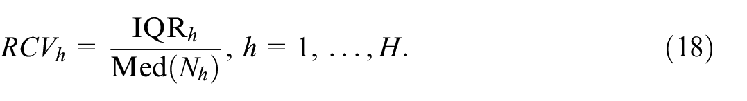
Results are shown in Figure 6. All values are below 8.4%; more than 90% of the municipalities have a $\mathrm{RCV}$ lower than 2%.

Figure 6.

Distribution of $\mathrm{RC}{V}_h$ (see Equation (18)) by region.

5. The Bayesian Model Applied to the 2018 Permanent Census Data

In the previous Section, we assessed our model performance using simulated data. In this Section, we analyze the real 2018 Permanent Census data. We implement the model described in Section 2 and detailed in Subsection 3.2 for every Italian region, using the 2018 Permanent Census data. Figure 7 shows the posterior mean of the probability of over (Figure 7a) and under-coverage (Figure 7b) at profile level averaged at a province level. Overall, over-coverage is the most relevant error source that the Base Register of Individuals (the administrative source) might be affected by; the province average ranges between 3% (Cuneo, PIE) and 15% (Siracusa, SIC), whereas the average under-coverage probability is always below 3.9% (Crotone, CAL).

Figure 7.

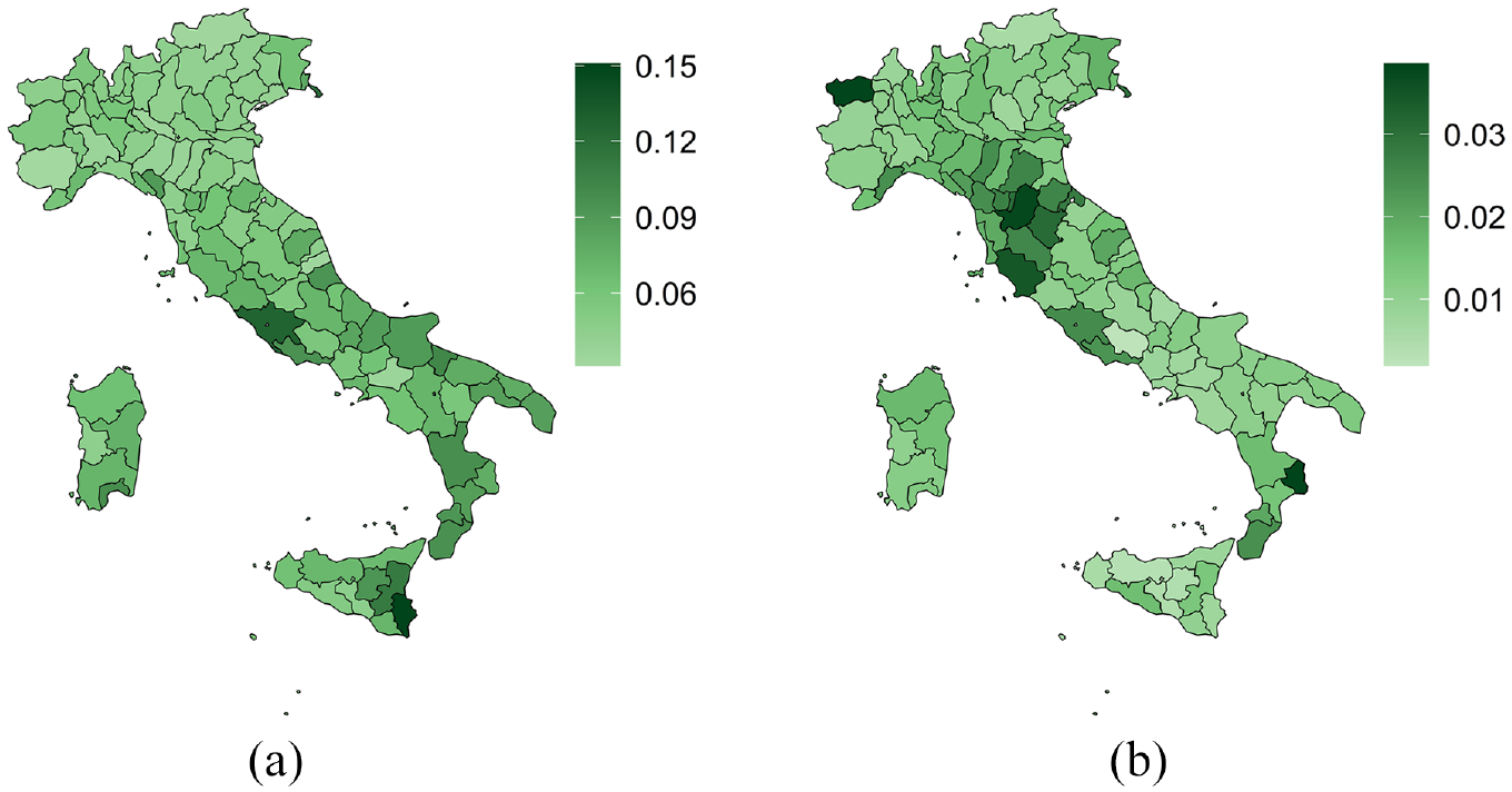
Over- and under-coverage probabilities at profile level, province averages. (a) Over-coverage and (b) under-coverage. 2018 Population census data.

The Appendix provides tables reporting the HPD95% of the $\mathbf{\beta }$ and $\mathbf{\delta }$ coefficients obtained for each region. Being a female or a non-Italian citizen is associated with a higher probability of being over-covered. For some regions, namely Calabria, Friuli-Venezia Giulia, Lombardia, Puglia, and Valle D’Aosta, being a foreign citizen is also associated with a higher under-coverage probability. The probability of being over-covered increases in the age classes of the most mobile (working) population, namely the third and the fourth ones, whereas there is a negative association with belonging to the last one, corresponding to the over-65 population.

Figure 8 shows the relative frequency of the inclusion of the count registered in the Base Register of the Individuals (BRI) in the HPD95% interval at the profile and municipal level. The relative frequency is quite high at the profile level, especially in Northern Italy, some provinces of the center and the South, and Sardegna (SAR). When we aggregate the results to a municipal level, the BRI count falls short of the more shrunk HPD95% interval. This may also be due to an error’s accumulation. At the municipality level, the error due to the model prediction is much lower than the coverage errors; at the profile level, the error in the models and the coverage errors have the same intensity and do not discriminate against each other. Figure 9 shows the same relative frequency of inclusion of the BRI count in the HPD95% interval, yet obtained using the simulated data.

Figure 8.

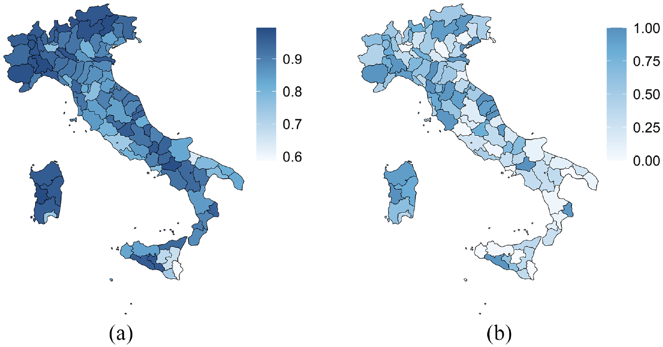
Relative frequency of the inclusion of the BRI estimate by the HPD95% at the profile and municipal level. Provincial average. 2018 Population census data. (a) Profile level and (b) municipal level.

Figure 9.

Relative frequency of the inclusion of the BRI estimate by the HPD95% at the profile and municipal level. Provincial average. Simulated data. (a) Profile level and (b) municipal level.

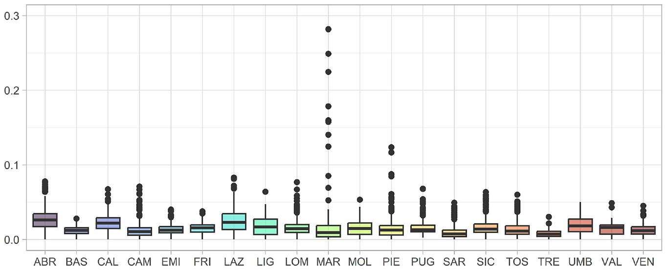
Finally, let us define the relative distance of the posterior median to the BRI estimate at the municipal level as

$${\Delta }_h(\mathcal{A},\mathrm{Med})=\frac{\mathrm{Med}\left(N_h\right)-N_h^{\mathcal{A}}}{N_h^{\mathcal{A}}},h=1,\dots ,H.$$

(19)

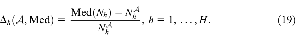
Figure 10 compares the regional distribution of ${\Delta }_h(\mathcal{A},\mathrm{Med})$ obtained using 2018 Population census data with that obtained using simulated data. The distributions are almost identical. All curves lie mainly on the negative values, exhibiting the weight of the over-coverage error in the administrative source. This strong similarity suggests that the evidence reported in the simulated data experiment can also be considered important for the application of the 2018 Population census data studied in this section.

Figure 10.

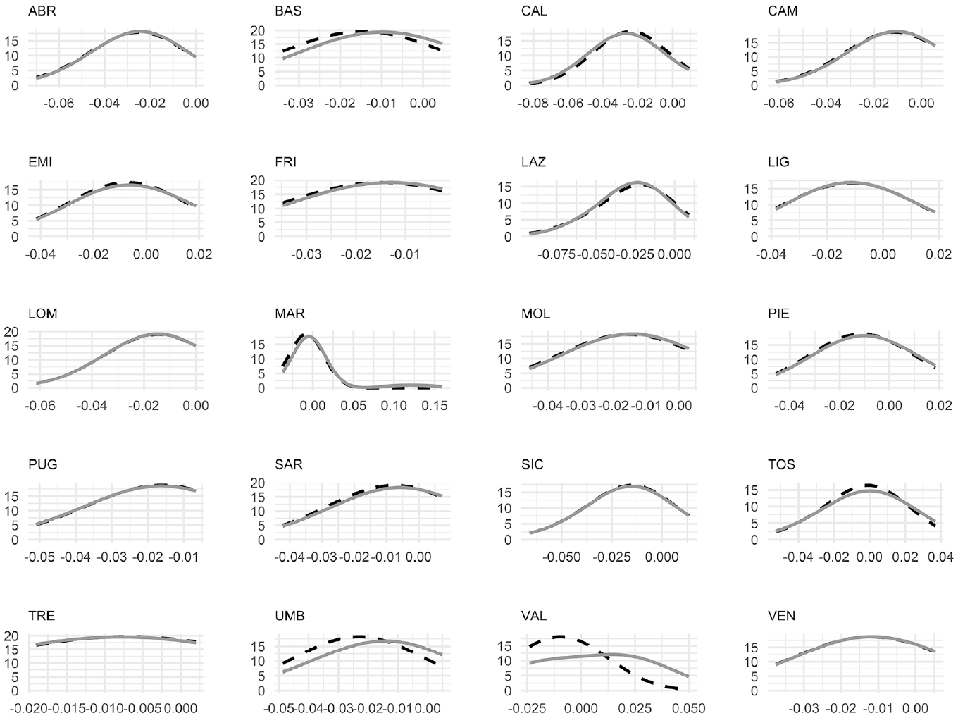
Relative distance between the municipal level posterior median, Med $\left(N_h\right)$ and the BRI estimate $N_h^{\mathcal{A}}$ . Real (black dashed curves) versus simulated (gray solid curves) data.

6. Conclusions

This paper proposes a Bayesian approach to estimating count data by integrating a nonprobability sample from an administrative source, which is susceptible to coverage errors, and two sample surveys. The proposed model provides count estimates at a detailed level, and it makes the uncertainty estimation straightforward. The application of this approach in a simulated experiment and to the 2018 Italian census data demonstrates its effectiveness in improving the quality of estimates by reducing bias in the administrative data source counts. Furthermore, it proves its feasibility in complex scenarios such as the Population Census.

However, it is important to note that the i.i.d. assumption used in the model approximation may not fully capture the random structure of the data due to survey design features such as stratification, weighting, and clustering. To address this limitation, future research should incorporate information on the sampling design into the modeling process to mitigate the effects of model misspecification. The inclusion of variables determining the sampling design as covariates and the use of hierarchical Bayesian models with random effects for clusters can enhance the accuracy of the estimates. Little (2006, 2022) offer valuable suggestions within a Bayesian framework to tackle this challenging problem. Di Zio et al. (2024) provides insights and proposals for considering sampling design features within the context of the application studied in this paper.

Finally, it is worth noting that errors other than under- and over-coverage ones, such as misclassification of the covariates defining the profiles, can also impact these data. Although misclassification is not accounted for in this study, it is essential to develop a general theoretical framework that simultaneously addresses misclassification and coverage errors. In the specific case of the Italian application, the influence of misclassification is deemed negligible for the variables used as covariates in the model. However, for a comprehensive approach, future work will aim to incorporate misclassification and coverage errors simultaneously, illustrating the flexibility of the model described in Section 2.