Performance Measures for Sample Selection Bias Correction by Weighting

Abstract

When estimating a population parameter by a nonprobability sample, that is, a sample without a known sampling mechanism, the estimate may suffer from sample selection bias. To correct selection bias, one of the often-used methods is assigning a set of unit weights to the nonprobability sample, and estimating the target parameter by a weighted sum. Such weights are often obtained with classification methods. However, a tailor-made framework to evaluate the quality of the assigned weights is missing in the literature, and the evaluation framework for prediction may not be suitable for population parameter estimation by weighting. We try to fill in the gap by discussing several promising performance measures, which are inspired by classical calibration and measures of selection bias. In this paper, we assume that the population parameter of interest is the population mean of a target variable. A simulation study and real data examples show that some performance measures have a strong positive relationship with the mean squared error and/or error of the estimated population mean. These performance measures may be helpful for model selection when constructing weights by logistic regression or machine learning algorithms.

1. Introduction

Probability samples have long been the gold standard for drawing reliable conclusions from the target population. However, probability samples often require much time and resources to collect. On the other hand, more and more naturally occurring data are available nowadays. For example, social media data, administrative data, or sensor data. These data sources are easier to collect in terms of time and cost or are already available due to digitalization (Cornesse et al. 2020). However, the inclusion mechanisms of these data sources are often unknown. Such data sets that have not been obtained through a known sampling mechanism are termed nonprobability samples. Without a known sampling mechanism, nonprobability samples are often treated as a simple random sample when estimating a population parameter (e.g., a population mean), and therefore may suffer from sample selection bias. When the inclusion mechanism of the nonprobability sample depends on the target variable we are interested in, selection bias is critical even with a large sample size (Meng 2018). For example, during the COVID-19 pandemic, an intensive survey was conducted by Facebook to investigate COVID-related features. Over 250,000 participants in the U.S. filled in the survey which was invited by the Facebook pop-on ad. The participants had a self-selection process after they saw the ad, and this process may have been affected by the COVID-related features. Although the number of participants was massive, the vaccination uptake rate was overestimated by 17% compared to the official figure. The large sample size also resulted in a narrow estimated variance so that the confidence interval could hardly cover the true value (Bradley et al. 2021).

Intensive research on selection bias correction methods has appeared. In general, selection bias correction methods can be categorized into $y$ -modeling (modeling the target variables), weighting, and combining $y$ -modeling and weighting (e.g., doubly robust estimation). See Elliott and Valliant (2017), Rao (2021), Wu (2022), and Meng (2022) for reviews. Here we focus on the weighting methods. In a weighting method, a set of unit weights is derived from, for example, inverse inclusion propensities (i.e., inclusion probabilities) or calibration given some estimated or known population values of auxiliary variables. The population parameter of interest is then estimated by a design-based estimator, for example, the Horvitz-Thompson estimator or Hájek estimator (Hájek 1971; Horvitz and Thompson 1952).

Such weights can be constructed in many different ways. The main aim of this paper is to select the best approach for constructing weights for a nonprobability sample out of a set of candidate approaches. However, a tailor-made model evaluation framework for the constructed weights is missing in the literature. Given the nature of selection bias correction frameworks, model evaluation methods for common statistical analyses, such as scoring rules in prediction (Gneiting and Raftery 2007), may not be suitable, since the interest is in having an unbiased estimated population parameter instead of a perfect unit-level prediction of the inclusion propensity. The relation between the constructed weights and the target variable will affect the performance of the weights (Meng 2018). For example, as an extreme case, if the target variable is a constant for every unit in the population, the performance of any constructed set of weights should be the same (assuming the weights sum up to the number of units in the population), while many often-used model evaluation indexes such as AIC fail to reflect this.

Besides, finding the correct propensity model for the nonprobability sample is not necessarily the goal when correcting for selection bias, similar to that it is not necessary to find the correct imputation model when imputing missing data (Vidotto et al. 2015). The inclusion mechanism of the nonprobability sample at hand may be unique. Without any strong reason, it is hard to believe that the acquired model can be applied to any other nonprobability sample. Having a correct model can assist in deriving many nice properties, as noted in Wu and Thompson (2020). However, it is hard to know even if the correct model exists or is considered in the candidate set of models (Zhang 2019). Instead of trying to find the correct model, we try to find the best model out of the candidate set of models by a performance measure. That is, a performance measure that reflects the underlying Mean Squared Error (MSE) and/or error of the estimated parameter. Ideally, that measure has a strong correlation with the MSE or error and we will be able to choose the best model based on the measure. We may then conduct variable selection or model selection, which is especially critical for the weighting method to prevent the variance of the correction method from outweighing the corrected bias. Literature suggests that only auxiliary variables that have strong relations with the target variable should be considered, while how to perform variable selection is not clear (Brick 2013; Mercer et al. 2017).

In the following sections, we will start by discussing the background in Section 2, and some possible performance measures for selection bias correction are described in Section 3. A simulation study and examples of real data sets will follow in Sections 4 and 5. Section 6 ends this article with a discussion and by drawing some conclusions.

2. Background

Before discussing the performance measures, it is useful to discuss the source of the selection bias and the mechanism of weighting methods. The discussion will focus on taking the population mean as the parameter of the target variable, while it can also be extended to more than one target variable or other parameters that are a linearizable function of the population mean.

2.1. Selection Bias

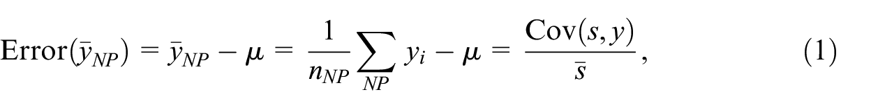
We assume that we are interested in a finite population ( $U$ ) with index $i\in \{1,2,\dots ,N\}$ . The population mean of the target variable $y$ , $\mu =N^{-1}\sum _U{y}_i$ , is the parameter of interest. We also assume that we have observed a nonprobability sample ( $\mathrm{NP}$ ) of size $n_{\mathrm{NP}}$ where $\mathrm{NP}\subset U$ . If $\mathrm{NP}$ is treated as a simple random sample without replacement from the population and used to estimate the population mean, the error in the nonprobability sample can be expressed as (Meng 2018)

$$\mathrm{Error}\left({\overline{y}}_{\mathrm{NP}}\right)={\overline{y}}_{\mathrm{NP}}-\mu =\frac{1}{n_{\mathrm{NP}}}\sum _{\mathrm{NP}}{y}_i-\mu =\frac{\mathrm{Cov}(s,y)}{\overline{s}},$$

(1)

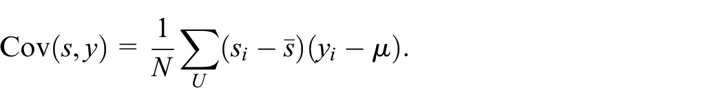
where $s$ is the inclusion indicator of the nonprobability sample, that is $s_i=1$ if $i\in \mathrm{NP}$ and 0 otherwise, and the population mean of the inclusion indicator $\overline{s}=N^{-1}\sum _U{s}_i$ . The population covariance of $s$ and $y$ is

$$\mathrm{Cov}(s,y)=\frac{1}{N}\sum _U(s_i-\overline{s})(y_i-\mu ).$$

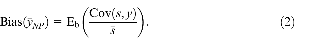
Assuming that the nonprobability sample is drawn from the population by means of some sampling mechanism ( $b$ ) with unknown inclusion propensities $\mathbb{P}(s_i=1)(i\in U)$ , we can find the bias of ( ${\overline{y}}_{\mathrm{NP}}$ ) by taking the expectation of Equation (1) over repeated sampling ( ${\mathrm{E}}_{\mathrm{b}}$ ). We then get

$$\mathrm{Bias}\left({\overline{y}}_{\mathrm{NP}}\right)={\mathrm{E}}_{\mathrm{b}}\left(\frac{\mathrm{Cov}(s,y)}{\overline{s}}\right).$$

(2)

Take the vaccination rate case in the Introduction as an example, the target variable $y_i$ is whether a person is vaccinated and $s_i$ is whether a person responds to the Facebook survey. If a vaccinated person has a higher or lower tendency to respond to the Facebook survey, selection error will occur in the estimated vaccination rate. Neither $\mathrm{Error}\left({\overline{y}}_{\mathrm{NP}}\right)$ nor $\mathrm{Bias}\left({\overline{y}}_{\mathrm{NP}}\right)$ can be estimated by the nonprobability sample only. Even if $\mathbb{P}(s_i=1)$ is known for units in $\mathrm{NP}$ , we still need to assume that the relationship between $s$ and $y$ in the nonprobability sample is the same as the relationship between $s$ and $y$ in the population (Nishimura et al. 2016).

2.2. Correcting Selection Bias by Weighting

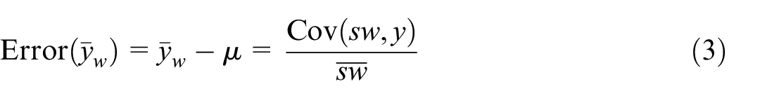
When correcting selection bias by weighting, often the target parameter $\mu$ is estimated by a design-based estimator ${\overline{y}}_w=\sum _{\mathrm{NP}}{w}_i{y}_i/\sum _{\mathrm{NP}}{w}_i$ where $w_i$ is a weight assigned to unit $i$ . The usage of a design-based estimator implies that we assume all units in the population have a non-zero probability of being included in the nonprobability sample. Our goal in this paper is to obtain a set of weights that minimizes $\mathrm{MSE}\left({\overline{y}}_w\right)={\mathrm{E}}_{\mathrm{b}}[{\overline{y}}_w-\mu {]}^2$ . Besides minimizing the MSE, it is often also of interest to minimize the error and the bias incurred in estimating the population mean. The error can be expressed as (Meng 2018, 2022)

$$\mathrm{Error}\left({\overline{y}}_w\right)={\overline{y}}_w-\mu =\frac{\mathrm{Cov}(\mathrm{sw},y)}{\overline{\mathrm{sw}}}$$

(3)

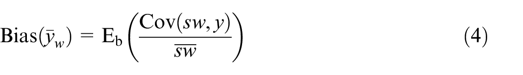
where $\overline{\mathrm{sw}}=N^{-1}\sum _U{s}_i{w}_i$ and the bias as

$$\mathrm{Bias}\left({\overline{y}}_w\right)={\mathrm{E}}_{\mathrm{b}}\left(\frac{\mathrm{Cov}(\mathrm{sw},y)}{\overline{\mathrm{sw}}}\right)$$

(4)

2.2.1. Construct Weights by Inverse Propensity Estimation

From Equation (4) we can see that the bias can be corrected if the constructed weights satisfy $w_i\propto \mathbb{P}{(s_i=1)}^{-1}$ , since then ${\mathrm{E}}_{\mathrm{b}}\left(s_i{w}_i\right)$ becomes a constant and therefore ${\mathrm{E}}_{\mathrm{b}}\left(\mathrm{Cov}(\mathrm{sw},y)\right)$ becomes zero no matter what the values of $y$ are. That is, if the true inclusion propensities are used, the bias vanishes for any target variable, similar to what normally happens in a design-based estimator. However, as mentioned in the Introduction, it is hard to know whether true inclusion propensities are obtained.

2.2.2. Construct Weights by Calibration

Besides propensity weighting, another often used correction method is calibration, see for example, Kim and Wang (2019), Chen et al. (2020), and Yang et al. (2020), and also a review in Wu (2022). Unlike inverse propensity weighting, it does not consider the underlying inclusion mechanism of the nonprobability sample but merely tries to obtain a set of weights that allows the weighted sum of the values of the target variable $y$ observed in the nonprobability sample to be equal or close to the population total of $y$ . The constructed weights are only valid for the target variable $y$ under consideration but are not necessarily valid for other target variables. To construct the weights, a set of auxiliary variables x with known or estimated population totals is needed. Ideally, the relations between the auxiliary variables and the target variable are strong so that if a set of weights can (approximately) obtain the known totals of the auxiliary variables, it can also assist in obtaining the population total of the target variable. The relation between $y$ and x can usually only be observed in the nonprobability sample. An assumption is needed that the relation between $y$ and x is the same when $s=1$ and $s=0$ so that f(y|x,s) = f(y|x) (at least approximately) given the empirical density function $f(·)$ for $y$ in the population or ℙ(s|x,y) = ℙ(s|x) (Little et al. 2020). Instead of directly constructing the weights by x, an alternative may be to fit the model ℙ(s|x,y) with ℙ(s|x,ŷ ) or $\mathbb{P}(s|\hat{y})$ . That is, construct the weights with the assistance of a model for $y$ . This $y$ -model should ideally be correctly specified (Marella 2023). Of course, the $y$ -model may not always be correctly specified. Later in the simulation we also explore the scenario when the $y$ -model is incorrect.

3. Performance Measures for Selection Bias Correction

In this section, we discuss some possible measures to evaluate a set of weights for selection bias correction. A performance measure is a nonnegative function of the weights, which has positive linear dependence with the mean squared error of the estimator of the finite population parameter of interest, constructed using these weights. That is, a measure that can give a good indication of the underlying unknown $\mathrm{MSE}\left({\overline{y}}_w\right)$ or $\mathrm{Error}\left({\overline{y}}_w\right)$ defined in Subsection 2.2. All the measures we present here are expected to have a positive relation with $\mathrm{MSE}\left({\overline{y}}_w\right)$ and/or absolute $\mathrm{Error}\left({\overline{y}}_w\right)$ .

The performance measures are presented under the two-sample setup, which has often been used in the selection bias correction literature, for example, Chen et al. (2020) and Elliott and Valliant (2017). In the two-sample setup, along with the nonprobability sample, a probability sample ( $P$ ) from the same population of size $n_P$ is available. For both $P$ and $\mathrm{NP}$ , the design weights $d_i=\mathbb{P}{(i\in P)}^{-1}$ and a common set of auxiliary variables x are available. Here we do not limit the possibility of whether the two samples are overlapping or not. The sample resulting by merging the nonprobability sample and the probability sample is denoted as $S_c$ so that the size of $S_c$ is $n=n_{\mathrm{NP}}+n_P$ , that is, overlapping units (if any) are counted twice.

3.1. Measures Without $y$ -Model

Here we discuss some measures that are often used for probability estimation or model evaluation in general. Since propensity estimation may be applied to construct weights, one may wonder whether performance measures for probability estimation will be helpful for evaluating the propensities.

In the following, we first discuss the mean cross entropy (MXE) and Brier score under the pseudo-weight method from Elliott and Valliant (2017). That pseudo-weight method first estimates ${\hat{\pi }}_i=\mathbb{P}(s_i=1|i\in S_c)$ and constructs the final weights with $w_i=d_i(1-{\hat{\pi }}_i)/{\hat{\pi }}_i$ , for details see Elliott and Valliant (2017). That is, the design weights of the probability sample are considered after modeling ${\hat{\pi }}_i$ , which allows the probability estimation methods to be applied in a standard way for estimating ${\pi }_i$ (i.e., without weighting the units by the design weights) and therefore many nonparametric or machine learning methods can be applied, for example, Bayesian Additive Regression Trees (BART) as proposed in Rafei et al. (2020, 2022; these articles also offer a broader discussion of estimation for nonprobability samples).

3.1.1. MXE

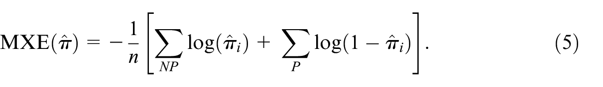
For MXE and Brier score the performance of the model is evaluated on ${\hat{\pi }}_i$ instead of the estimated propensity to be included in the nonprobability sample ${\hat{p}}_i=1/w_i$ , since the goal is to minimize the impurity of the estimated ${\hat{\pi }}_i$ but not of the underlying propensities. MXE under the two-sample setup is (Caruana and Niculescu-Mizil 2004; Kullback 1997),

$$\mathrm{MXE}\left(\hat{\pi }\right)=-\frac{1}{n}[\sum _{\mathrm{NP}}\log \left({\hat{\pi }}_i\right)+\sum _P\log (1-{\hat{\pi }}_i)].$$

(5)

A smaller value for MXE indicates better performance according to this measure. So, ${\hat{\pi }}_i$ closer to 0 or 1 will be preferable by MXE.

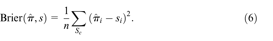
3.1.2. Brier’s Score

A similar measure is Brier’s score which is a distance-based measure. A smaller value of the Brier score reflects a smaller distance between the ${\hat{\pi }}_i$ and the $s_i$ and therefore ${\hat{\pi }}_i$ close to 0 or 1 is also preferred. The formula is (Brier 1950)

$$\mathrm{Brier}(\hat{\pi },s)=\frac{1}{n}\sum _{S_c}{({\hat{\pi }}_i-s_i)}^2.$$

(6)

3.1.3. AIC

For model selection, the Akaike information criterion (AIC) is one of the often-used measures (Akaike 1974; Schwarz 1978). AIC is based on the value of the likelihood function $\hat{L}$ of the estimated model with a penalty on the used number of parameters ( $k$ ) of the model,

$$\mathrm{AIC}(k,\hat{L})=2k-2\ln \left(\hat{L}\right).$$

(7)

An AIC for complex design survey data has also been proposed by Lumley and Scott (2015). For many machine learning methods, it is difficult or even impossible to calculate AIC since the likelihood function is unknown, and sometimes even the number of parameters is unknown as well (e.g., a tree model).

3.1.4. Cal1

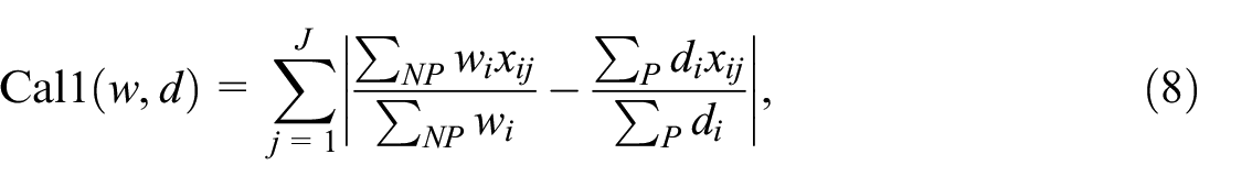
As noted in Subsection 2.2, calibration is an often-used method for selection bias correction. The calibration property may be suitable for not only constructing the weights but also serving as a performance measure. Based on the calibration property, we may examine the performance of the weights by auxiliary variables which are strongly correlated to the target variable (Deville and Särndal 1992). If the differences between weighted totals of the auxiliary variables and the corresponding known totals are small, we may conclude that we have a good set of weights. Under the two-sample setup, the population means of the auxiliary variables can be estimated from the probability sample by $\sum _p{d}_i{\mathit{x}}_i/\sum _p{d}_i$ . Therefore we can calculate

$$\mathrm{Cal}1(w,d)=\sum _{j=1}^J|\frac{\sum _{\mathrm{NP}}{w}_i{x}_{\mathrm{ij}}}{\sum _{\mathrm{NP}}{w}_i}-\frac{\sum _P{d}_i{x}_{\mathrm{ij}}}{\sum _P{d}_i}|,$$

(8)

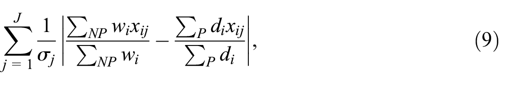
which is the sum of the absolute differences between the weighted and design-based estimates of the population means over $J$ auxiliary variables from the two samples. A set of weights with the smallest value of Cal1 will then be chosen. This approach has been applied by Yang et al. (2020) as a loss function for weight construction and as a performance measure for tuning. Since Cal1 is sensitive to the scale of the auxiliary variables, it may be standardized by

$$\sum _{j=1}^J\frac{1}{{\sigma }_j}|\frac{\sum _{\mathrm{NP}}{w}_i{x}_{\mathrm{ij}}}{\sum _{\mathrm{NP}}{w}_i}-\frac{\sum _P{d}_i{x}_{\mathrm{ij}}}{\sum _P{d}_i}|,$$

(9)

where ${\sigma }_j$ is the standard deviation of $x_j$ and may be estimated by ${(({\sigma }_{j,\mathrm{NP}}^2+{\sigma }_{j,P}^2)/2)}^{0.5}$ . ${\sigma }_{j,\mathrm{NP}}^2$ and ${\sigma }_{j,P}^2$ are the estimated variances of $x_j$ from the nonprobability sample and the probability sample, where ${\sigma }_{j,\mathrm{NP}}^2$ is estimated by assuming that $\mathrm{NP}$ was obtained by a simple random sample, which may not be a realistic assumption in practice. Equation (9) has been applied in McCaffrey et al. (2004), Austin (2009), and Kern et al. (2021).

3.2. Measures With $y$ -Model

3.2.1. Cal2 and Cal3

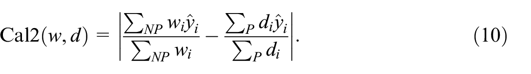
As noted in Section 2, it may be useful to also consider a $y$ -model when using the weighting approach. The first two measures with $y$ -models that we consider are transformations of Equation (8). An underlying assumption of Equation (8) and Equation (9) is that the auxiliary variables and the target variable have a linear relation, which may not be met in practice (Deville and Särndal 1992). As an alternative, Wu and Sitter (2001) proposed a model-calibration method that allows all types of relationships between the auxiliary variables and the target variable. Rather than using x as in Equation (8), a model $\hat{y}=\hat{m}(\mathbf{x})$ is fitted on the nonprobability sample, where $\hat{m}(·)$ can be any function. The weights are then evaluated by the weighted total of $\hat{y}$ in the two samples, that is, the performance measure will be

$$\mathrm{Cal}2(w,d)=|\frac{\sum _{\mathrm{NP}}{w}_i{\hat{y}}_i}{\sum _{\mathrm{NP}}{w}_i}-\frac{\sum _P{d}_i{\hat{y}}_i}{\sum _P{d}_i}|.$$

(10)

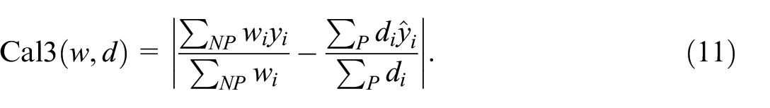
We also look at the difference between the weighted sum of the observed $y$ and the weighted sum of $\hat{y}$ ,

$$\mathrm{Cal}3(w,d)=|\frac{\sum _{\mathrm{NP}}{w}_i{y}_i}{\sum _{\mathrm{NP}}{w}_i}-\frac{\sum _P{d}_i{\hat{y}}_i}{\sum _P{d}_i}|.$$

(11)

With the usage of $y$ in the nonprobability sample, Equation (11) may be less subject to model misspecification compared to Equation (10).

3.2.2. MSB

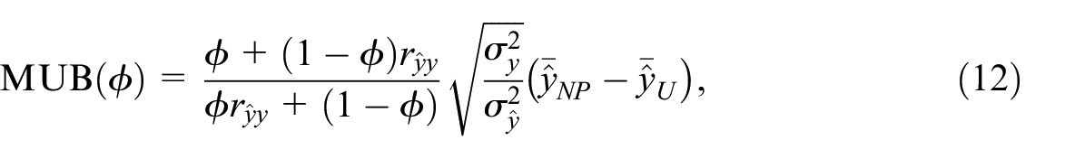
One way to estimate the selection bias is the Measure of Unadjusted Bias (MUB) proposed by Little et al. (2020), which may also be useful for evaluating the performance of the acquired weights. In Boonstra et al. (2021), it is shown that MUB outperforms other measures such as the R-indicator, Coefficient of Variation (CV), or Area Under the receiver-operating characteristic Curve (AUC; for details on these measures, see Boonstra et al. 2021) in reflecting the amount of selection bias. MUB aims to estimate ${\overline{y}}_{\mathrm{NP}}-\mu$ by assuming the inclusion mechanism is from a function of ℙ(s = 1|x,y) = g[(1 −ϕ)ŷ+ϕy], where $\varphi \in [0,1]$ is an unknown model parameter that allows different degrees of ignorability to be considered, and $g[·]$ is some function. A model $\hat{y}=\hat{m}(\mathbf{x})$ is fitted on the nonprobability sample, and $\hat{m}(\mathbf{x})$ is used in the probability sample to calculate $\hat{y}$ . When $\varphi =1$ , $\mathrm{MUB}\left(\varphi \right)$ completely depends on the observed $y$ in the nonprobability sample, and when $\varphi =0$ , $\mathrm{MUB}\left(\varphi \right)$ completely depends on $\hat{y}$ , which is aligned with Cal3, see Little et al. (2020) for details. The definition of $\mathrm{MUB}\left(\varphi \right)$ under the two-sample setup is

$$\mathrm{MUB}\left(\varphi \right)=\frac{\varphi +(1-\varphi )r_{\hat{y}y}}{\varphi r_{\hat{y}y}+(1-\varphi )}\sqrt{\frac{{\sigma }_y^2}{{\sigma }_{\hat{y}}^2}}({\overline{\hat{y}}}_{\mathrm{NP}}-{\overline{\hat{y}}}_U),$$

(12)

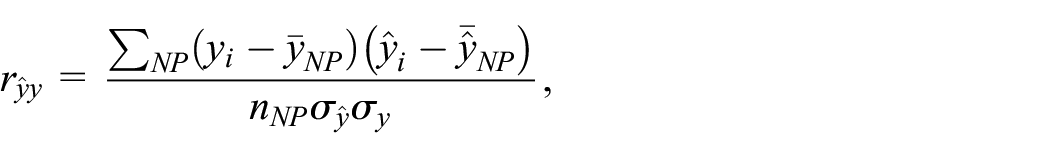
where ${\overline{\hat{y}}}_{\mathrm{NP}}=n_{\mathrm{NP}}^{-1}\sum _{\mathrm{NP}}{\hat{y}}_i$ , ${\overline{\hat{y}}}_U=\sum _P{d}_i{\hat{y}}_i/\sum _P{d}_i$ , $r_{\hat{y}y}$ is the correlation coefficient of $\hat{y}$ and $y$ , that is,

$$r_{\hat{y}y}=\frac{\sum _{\mathrm{NP}}(y_i-{\overline{y}}_{\mathrm{NP}})({\hat{y}}_i-{\overline{\hat{y}}}_{\mathrm{NP}})}{n_{\mathrm{NP}}{\sigma }_{\hat{y}}{\sigma }_y},$$

and ${\sigma }_y^2$ , ${\sigma }_{\hat{y}}^2$ are estimated by ${\hat{\sigma }}_y^2=n_{\mathrm{NP}}^{-1}\sum _{\mathrm{NP}}{(y_i-{\overline{y}}_{\mathrm{NP}})}^2$ and ${\hat{\sigma }}_{\hat{y}}^2=n_{\mathrm{NP}}^{-1}\sum _{\mathrm{NP}}{({\hat{y}}_i-{\overline{\hat{y}}}_{\mathrm{NP}})}^2$ . Note that in this setup we assume that the auxiliary variables used to obtain $\hat{y}$ are not available outside of the two samples. If the population totals of the auxiliary variables are available, MUB may give a more accurate error estimation since using the estimated population value is naturally losing efficiency compared to a known population parameter (Zhang 2019). A performance measure that borrows the strength of $\mathrm{MUB}\left(\varphi \right)$ may be:

$$\mathrm{MSB}\left(\varphi \right)\equiv |\mathrm{MUB}\left(\varphi \right)-{\overline{y}}_{\mathrm{NP}}+{\overline{y}}_w|.$$

(13)

That is, if the difference between the naive estimate ${\overline{y}}_{\mathrm{NP}}$ for $y$ and the weighted mean ${\overline{y}}_w$ is close to $\mathrm{MUB}\left(\varphi \right)$ , we may conclude that the acquired set of weights can correct the underlying selection bias.

It is worth noting that, since $\mu$ is fixed, ${\overline{y}}_w$ naturally has a perfect positive relationship with $\mathrm{Error}\left({\overline{y}}_w\right)$ , see Equation (3). We can have an idea of the direction of the error by merely looking at whether the estimated ${\overline{y}}_w$ is moving away from or toward ${\overline{y}}_{\mathrm{NP}}$ . However, merely looking at ${\overline{y}}_w$ does not prevent us from over-correction, that is, when ${\overline{y}}_{\mathrm{NP}}-\mu$ has an opposite sign to $\mathrm{Error}\left({\overline{y}}_w\right)$ . We hope to understand whether the selection error is over-corrected by considering the $\mathrm{MUB}\left(\varphi \right)$ in the measure. If $\mathrm{Error}\left({\overline{y}}_w\right)$ is zero, ideally the value of MSB should also be zero.

3.2.3. KS

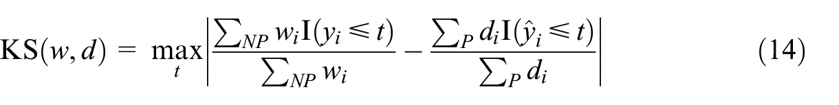
Another model evaluation index in the nonresponse literature is the Kolmogorov-Smirnov (KS) distance (Chambers 2001). KS distance is a non-parametric index that calculates the maximum difference between two empirical cumulative distribution functions. Unlike AIC, KS can be applied to the result from any model. Under the two-sample setup, we calculate the maximum difference by

$$\mathrm{KS}(w,d)=\underset{t}{\max }|\frac{\sum _{\mathrm{NP}}{w}_i\mathrm{I}(y_i\le t)}{\sum _{\mathrm{NP}}{w}_i}-\frac{\sum _P{d}_i\mathrm{I}({\hat{y}}_i\le t)}{\sum _P{d}_i}|$$

(14)

for $t\in (-\infty ,\infty )$ , where $\mathrm{I}(·)$ is an indicator function.

4. Simulation

4.1. Simulated Data

We evaluate the performance measures by examining the relation of the performance measures with $\mathrm{MSE}\left({\overline{y}}_w\right)$ and absolute $\mathrm{Error}\left({\overline{y}}_w\right)$ . A population of size 10,000 with auxiliary variables $x_1,x_2,x_3,x_4~N(1,1)$ is created. The target variable $y=3x_1+x_2-5x_3+0.1x_4+e$ , where $e~N(0,1)$ . The finite population mean of $y$ is $\mu \approx -0.9$ . The auxiliary variables are available both for the probability and nonprobability samples while the target variable is only available in the nonprobability sample. The probability sample is repeatedly drawn by means of simple random sampling without replacement with inclusion probability $0.05$ , that is, $d=20$ is the design weight for all units in the probability sample, and results in $n_P=500$ . The nonprobability sample is repeatedly drawn by means of fixed-size unequal probability sampling without replacement. We do this by randomized systematic sampling with inclusion probability $p=\exp (c+x_1+x_2-0.5x_3)/(1+\exp (c+x_1+x_2-0.5x_3))$ , where $c$ is a constant so that the inclusion fraction of the nonprobability sample is fixed at $0.1$ , which results in $n_{\mathrm{NP}}=1,000$ (Madow 1949). The result of a nonlinear propensity model $p=\exp (c+x_1+0.5x_2{x}_4)/(1+\exp (c+x_1+0.5x_2{x}_4))$ is shown in Appendix A, which shows a similar conclusion as the linear one.

4.2. Estimation and Evaluation

The weights are constructed by Elliott and Valliant’s (2017) pseudo-weight method as discussed in Subsection 3.1, since Elliott and Valliant’s method offers a relatively stable estimation compared to methods considering design weights during the propensity model estimation (Liu et al. 2023). To reflect different possible model choices, the propensity model ${\hat{\pi }}_i=\mathbb{P}(s_i=1|i\in S_c)$ is fitted by a machine learning algorithm, XGBoost, and logistic regression (Chen and Guestrin 2016).

XGBoost is a flexible and powerful algorithm in prediction problems, and it has been applied in Castro-Martín et al. (2020) and Klingwort and Burger (2023) for selection bias correction. As for many machine learning algorithms, hyperparameters should be chosen before fitting the XGBoost model (see, e.g., Chen and Guestrin 2016 for these hyperparameters). In the simulation, we use the default hyperparameters in XGBoost. A more detailed tuning scheme will be performed later in the real data examples. Note that the AIC cannot be calculated for XGBoost since the number of parameters and the likelihood function are unknown.

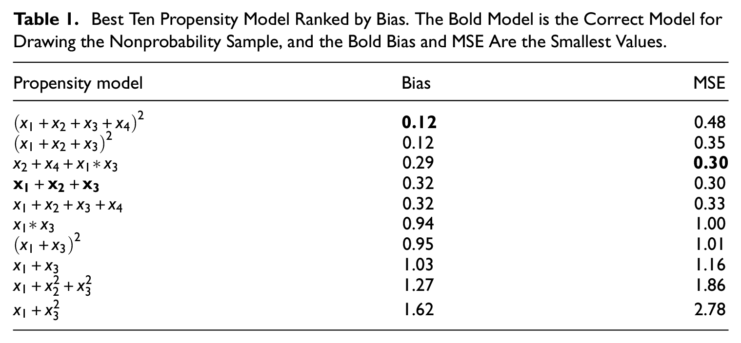
For logistic regression, the correct model and thirty-three incorrectly specified or over-specified models are fitted. These incorrectly specified or over-specified models, for example, miss some auxiliary variables, have some extra interactions between variables, or have higher-order terms of the variables. The incorrectly specified models may reflect the effect of a Not Missing At Random mechanism. See Supplemental Material for details on the models used or Table 1 for a few examples.

Table 1.

Best Ten Propensity Model Ranked by Bias. The Bold Model is the Correct Model for Drawing the Nonprobability Sample, and the Bold Bias and MSE Are the Smallest Values.

Propensity model	Bias	MSE
${(x_1+x_2+x_3+x_4)}^2$	0.12	0.48
${(x_1+x_2+x_3)}^2$	0.12	0.35
$x_2+x_4+x_1*x_3$	0.29	0.30
${\mathbf{x}}_1+{\mathbf{x}}_2+{\mathbf{x}}_3$	0.32	0.30
$x_1+x_2+x_3+x_4$	0.32	0.33
$x_1*x_3$	0.94	1.00
${(x_1+x_3)}^2$	0.95	1.01
$x_1+x_3$	1.03	1.16
$x_1+x_2^2+x_3^2$	1.27	1.86
$x_1+x_3^2$	1.62	2.78

In total, thirty-five models/methods are used to estimate the propensity scores to reflect the relation between the measures and different degrees of the estimated MSE of the estimated population mean, which is $\widehat{\mathrm{MSE}}\left({\overline{y}}_w\right)=R^{-1}\sum _{r=1}^R{[{\overline{y}}_{w,r}-\mu ]}^2,$ where ${\overline{y}}_w=\sum _{\mathrm{NP}}{w}_i{y}_i/\sum _{\mathrm{NP}}{w}_i$ , and $R=1,000$ is the number of replicates in drawing a probability and non-probability sample. The averages of the performance measures under each model are recorded.

For measures considering a $y$ -model as in Subsection 3.2, we apply linear regression with the correct model (using $x_1,x_2,x_3,x_4$ as the auxiliary variables) and an incorrect model (using $x_2$ and $x_4$ only) to show the effect of different model use. The adjusted $R^2$ of the correct model in the nonprobability sample is around .967, and the adjusted $R^2$ of the incorrect model is around .011.

4.3. Results

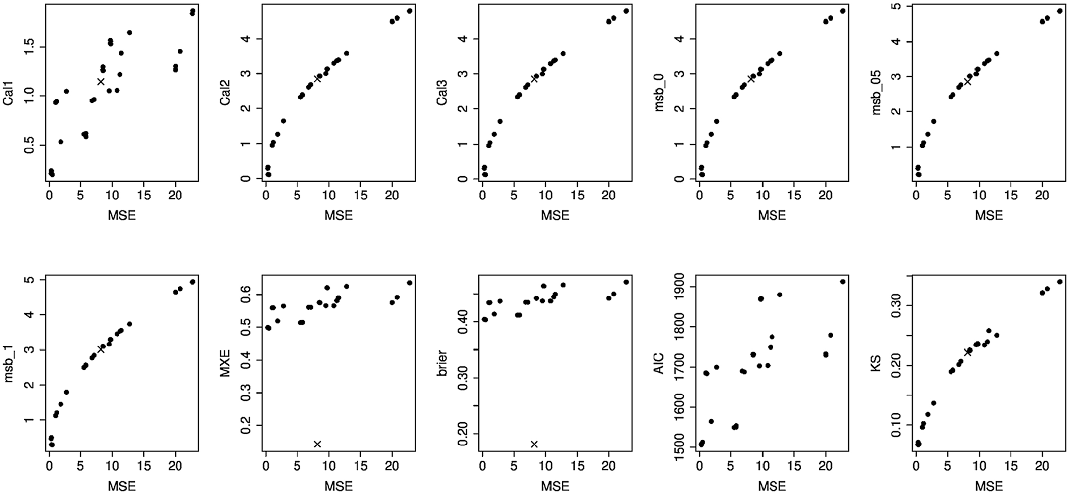
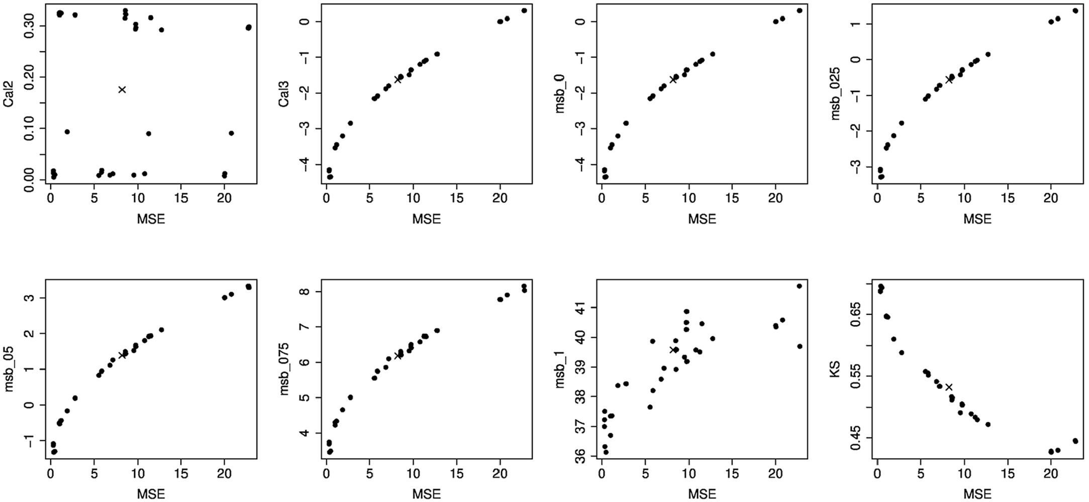
Figures 1 and 2 show the relations between each measure and $\widehat{\mathrm{MSE}}\left({\overline{y}}_w\right)$ for the thirty-five specified models. The number after MSB is the value of $\varphi$ , for example, MSB05 indicates that $\varphi =0.5$ is used. Figure 1 shows that in general all measures are positively related to $\widehat{\mathrm{MSE}}\left({\overline{y}}_w\right)$ under the correct $y$ -model. Figure 2 shows the effect of an incorrect $y$ -model, therefore only measures with a $y$ -model are shown. For Cal2, the relation is only clear when the correct $y$ -model is used, while under the incorrect $y$ -model, a low correlation between Cal2 and $\widehat{\mathrm{MSE}}\left({\overline{y}}_w\right)$ is observed. Cal3 and MSB0 show the opposite relation between the measures and $\widehat{\mathrm{MSE}}\left({\overline{y}}_w\right)$ . However, if the unknown parameter $\varphi$ is well chosen, between $0.5$ and $0.75$ in this case, zero estimated MSB is then corresponding to zero $\widehat{\mathrm{MSE}}\left({\overline{y}}_w\right)$ . KS has a negative relation with $\widehat{\mathrm{MSE}}\left({\overline{y}}_w\right)$ when the wrong $y$ -model is applied.

Figure 1.

Relations between $\widehat{\mathrm{MSE}}\left({\overline{y}}_w\right)$ and the mean performance measures under different propensity model specifications. The correct $y$ -model is used. The dots are the estimates from logistic regression and the cross is the estimate from XGBoost. Measures include different variants of calibration (Cal1, Cal2, Cal3), measure of selection bias (MSB) with different $\varphi$ , Mean cross entropy (MXE), Brier score, Akaike information criterion (AIC), and Kolmogorov-Smirnov distance (KS).

Figure 2.

Relations between $\widehat{\mathrm{MSE}}\left({\overline{y}}_w\right)$ and mean performance measures when the incorrect $y$ -model is used. The dots are the estimates from logistic regression and the cross is the estimate from XGBoost. Measures with a $y$ -model include two variants of calibration (Cal2, Cal3), measure of selection bias (MSB) with different $\varphi$ , and Kolmogorov-Smirnov distance (KS).

MXE and Brier have a similar tendency since $\hat{\pi }$ is mostly around $0.7$ and the difference between these performance measures will only be obvious when the estimated probability is close to 0 or 1. XGBoost indeed gives a good estimation in terms of impurity (low MXE and Brier), however, low impurity does not necessarily guarantee a good population parameter estimate. In fact, when the estimated propensity is close to $0$ , although this results in a low impurity, this also causes a large weight and a large variation of the parameter estimates.

In Table 1 we list the best ten models in terms of $\mathrm{Bias}=R^{-1}\sum _{r=1}^R{\overline{y}}_{w,r}-\mu$ . It is interesting to see that the correct propensity model does not necessarily perform the best in terms of both Bias and MSE. Some overfitting models may capture the underlying variation and allow a better parameter estimation. A similar discussion can also be found in the imputation literature, see, for example, Vermunt et al. (2008) and Vidotto et al. (2015).

4.4. Selecting Smallest Error

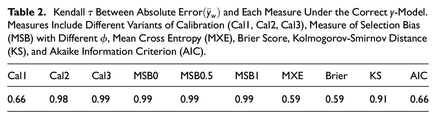
We also examine whether the performance measures are able to pick out the best model in terms of absolute $\mathrm{Error}\left({\overline{y}}_w\right)$ . In every set of the drawn samples, thirty-five models are fitted as before. Kendall rank correlation coefficient ( $\tau$ ) between absolute $\mathrm{Error}\left({\overline{y}}_w\right)$ of the thirty-five models and each measure is calculated to reflect whether the measures are able to rank the models correctly (Kendall 1948). Kendall $\tau$ is calculated by the probability of the same order of pairs of two units of a variable, subtracting the probability of different order of pairs of two units, that is, how consistent the orders between the two variables are (here the performance measure and absolute Error). Kendall $\tau =1$ if two variables share the same rank, and $\tau =-1$ if two variables have totally opposite rankings. That is, if $\tau =1$ for a performance measure and absolute $\mathrm{Error}\left({\overline{y}}_w\right)$ , it means that in every possible subset of the thirty-five models, we will be able to pick out the best model based on the value of the performance measure. The averages of $\tau$ for all measures over a thousand runs are reported.

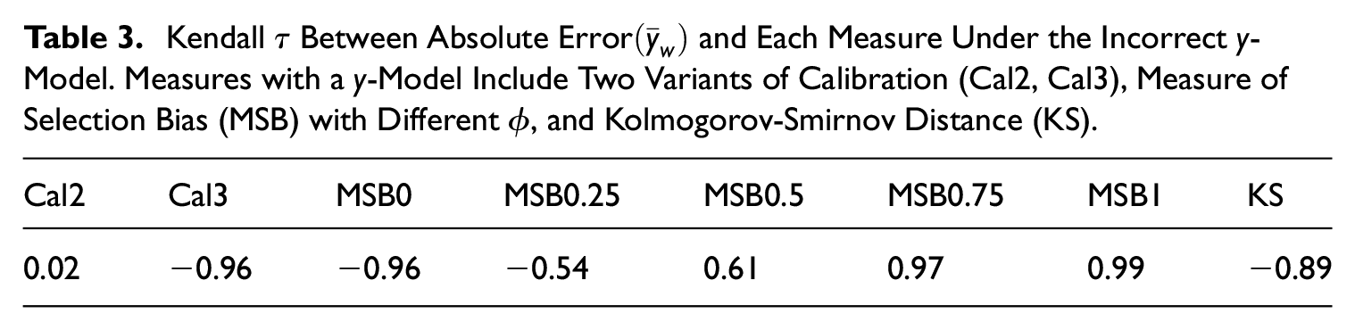
Tables 2 and 3 show the average Kendall rank correlation coefficient between absolute $\mathrm{Error}\left({\overline{y}}_w\right)$ and each measure. In general, measures considering a $y$ -model are strongly correlated with the actual underlying error, that is, we are able to pick out the smallest error model based on Cal2, Cal3, MSB, and KS under the correct $y$ -model. Under the incorrect $y$ -model, only MSB with $\varphi \in [0.75,1]$ may give a good indication.

Table 2.

Kendall $\tau$ Between Absolute $\mathrm{Error}\left({\overline{y}}_w\right)$ and Each Measure Under the Correct $y$ -Model. Measures Include Different Variants of Calibration (Cal1, Cal2, Cal3), Measure of Selection Bias (MSB) with Different $\varphi$ , Mean Cross Entropy (MXE), Brier Score, Kolmogorov-Smirnov Distance (KS), and Akaike Information Criterion (AIC).

Cal1	Cal2	Cal3	MSB0	MSB0.5	MSB1	MXE	Brier	KS	AIC
0.66	0.98	0.99	0.99	0.99	0.99	0.59	0.59	0.91	0.66

Table 3.

Kendall $\tau$ Between Absolute $\mathrm{Error}\left({\overline{y}}_w\right)$ and Each Measure Under the Incorrect $y$ -Model. Measures with a $y$ -Model Include Two Variants of Calibration (Cal2, Cal3), Measure of Selection Bias (MSB) with Different $\varphi$ , and Kolmogorov-Smirnov Distance (KS).

Cal2	Cal3	MSB0	MSB0.25	MSB0.5	MSB0.75	MSB1	KS
0.02	−0.96	−0.96	−0.54	0.61	0.97	0.99	−0.89

5. Experiments on Real Data Sets

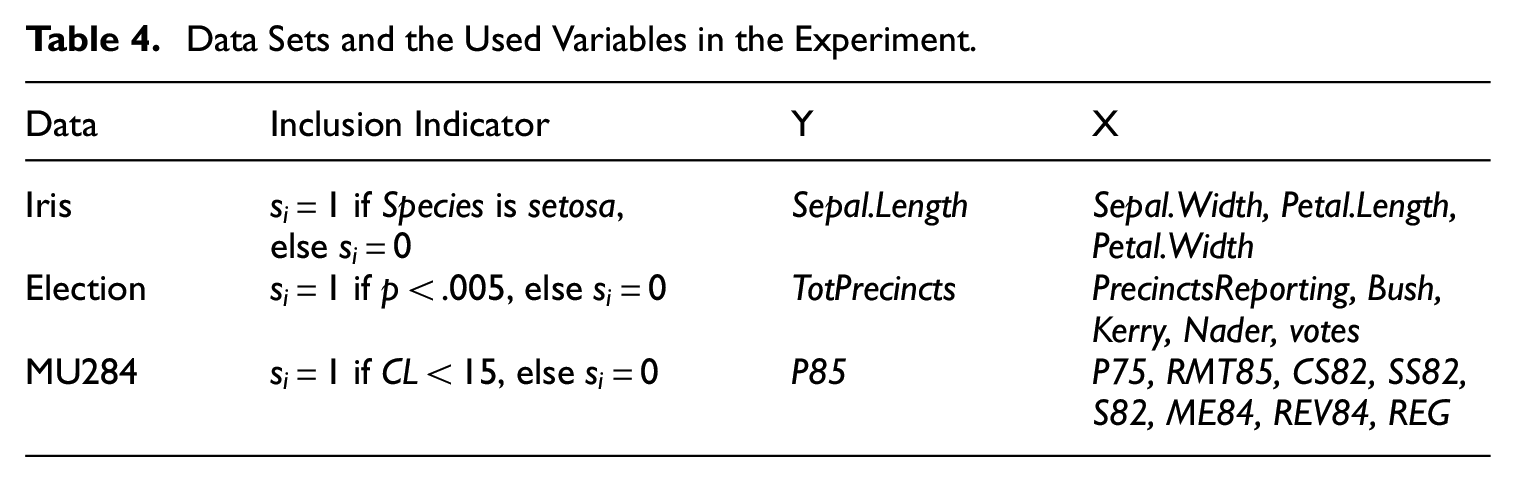
The experiment looks at the performance measures under various real data sets. Since in practice the true models for target variable $y$ and the inclusion mechanism of the nonprobability sample are usually unknown to the investigator, we try to mimic this situation in the experiment. Three data sets in R packages are used, that is, Iris data (Anderson 1935), Election data from the Survey package (Lumley 2020), and MU284 data from the Sampling package (Tillé and Matei 2021). See the references therein for the details of the data sets. These data sets are treated as populations where one of the variables is treated as the indicator of inclusion in the nonprobability sample, one continuous variable is treated as the target variable of which the population mean is of interest, and the rest of the variables are the auxiliary variables. The variable specification is shown in Table 4.

Table 4.

Data Sets and the Used Variables in the Experiment.

Data	Inclusion Indicator	Y	X
Iris	$s_i=1$ if Species is setosa, else $s_i=0$	Sepal.Length	Sepal.Width, Petal.Length, Petal.Width
Election	$s_i=1$ if p < .005, else $s_i=0$	TotPrecincts	PrecinctsReporting, Bush, Kerry, Nader, votes
MU284	$s_i=1$ if CL < 15, else $s_i=0$	P85	P75, RMT85, CS82, SS82, S82, ME84, REV84, REG

Since the propensity model of the nonprobability sample is unknown in this case, we may only look at absolute $\mathrm{Error}\left({\overline{y}}_w\right)$ but not $\mathrm{MSE}\left({\overline{y}}_w\right)$ . A simple random sample with an inclusion fraction of $0.1$ is drawn from the population and treated as the available probability sample. The construction of the weights is again the pseudo-weight method from Elliott and Valliant (2017) where XGBoost is used for the propensity estimation. We grid search a range of tuning parameters of XGBoost under reasonable ranges including

• Learning rate ( $\eta$ ): Learning rate is between 0 and 1, and the default value is 0.3. A higher learning rate means a larger contribution of each tree. A set of $\{0,0.3,0.5,0.7\}$ is used.

• Minimum loss ( $\gamma$ ): The minimum loss that needs to be reduced when partitioning. It ranges from 0 to $\infty$ and the default value is 0. Here we use $\{0,1,2\}$ .

• Minimum child weight: The minimum of the sum of weights in a child node. It ranges from 0 to $\infty$ and the default value is 1. $\{1,3,5,7\}$ is used.

In total, there are $4\times 3\times 4=48$ combinations of the tuning parameters. $\mathrm{Error}\left({\overline{y}}_w\right)$ of each combination is calculated, and the relations between $\mathrm{Error}\left({\overline{y}}_w\right)$ and the measures are shown. Note that, unlike a prediction task, we do not use cross-validation for tuning since the goal is not to find a model for future prediction but to estimate population parameters by means of the probability sample and the nonprobability sample. The $y$ -model is fitted by linear regression, using all the auxiliary variables as predictors.

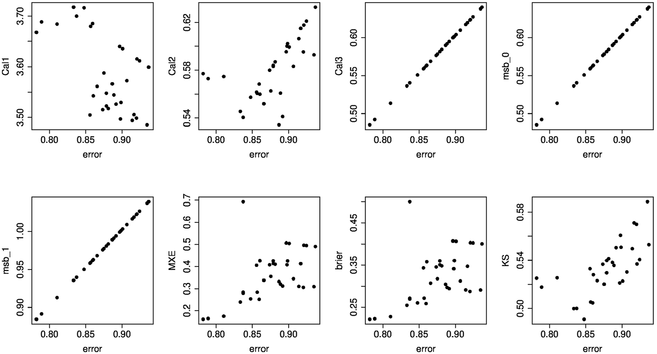
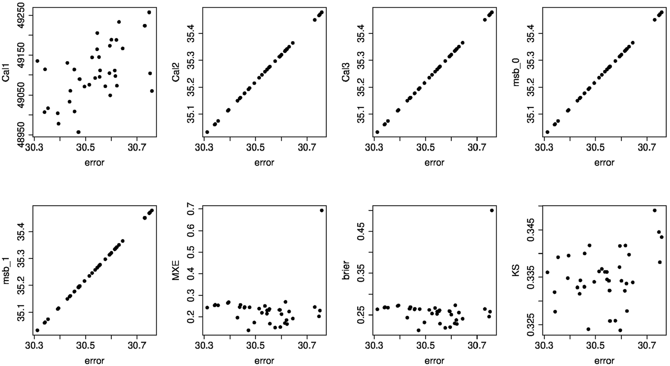
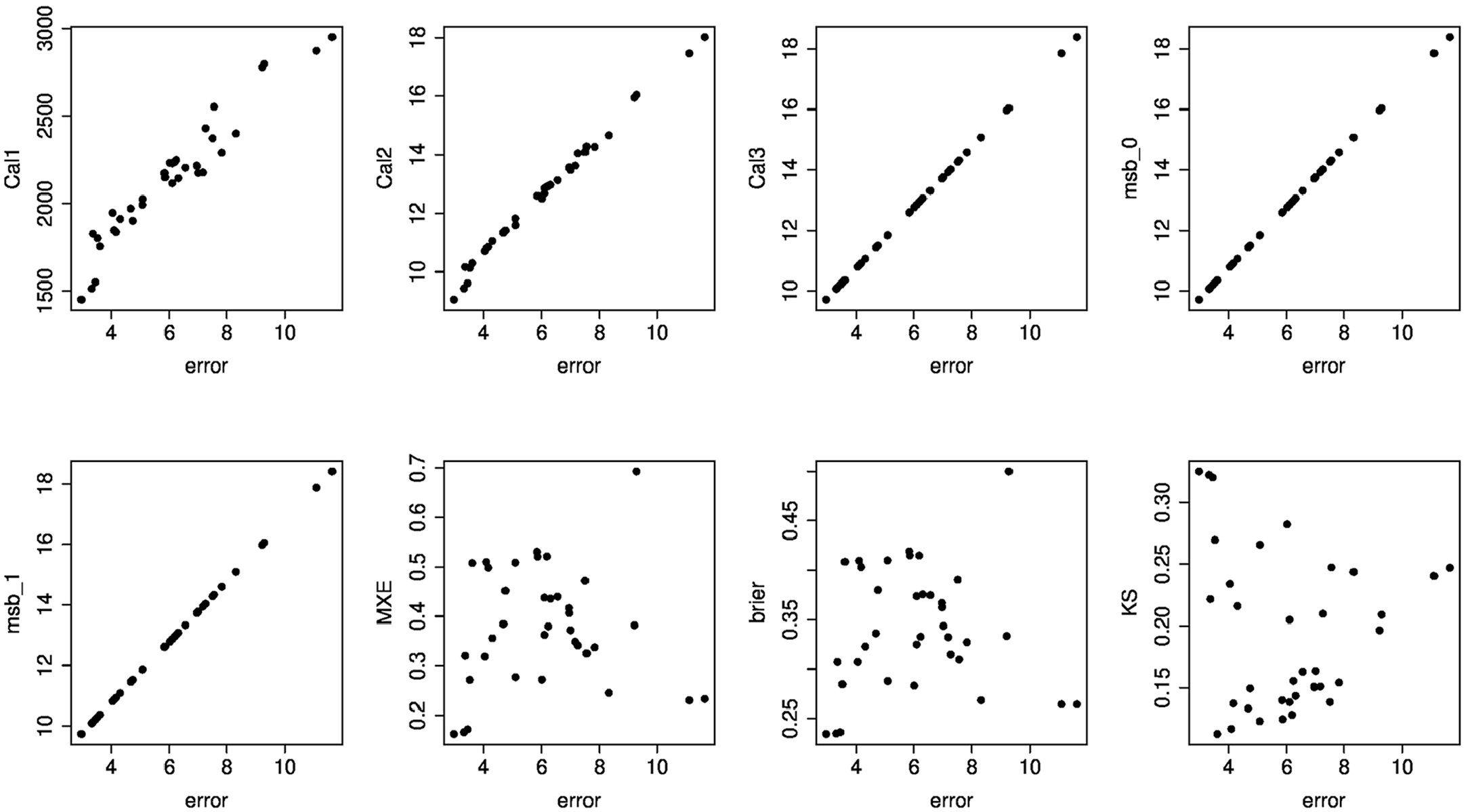
Figures 3 to 5 show the relationships between the performance measures and absolute $\mathrm{Error}\left({\overline{y}}_w\right)$ . In general, the patterns are similar to those in the simulation. The measures with a $y$ -model for target variable $y$ better reflect the underlying absolute $\mathrm{Error}\left({\overline{y}}_w\right)$ . It also can be seen that the three data sets offer sufficient auxiliary information so that Cal2, Cal3, and MSB reflect clear indications of model performance, while Cal1 may not be useful when some auxiliary variables have a negative correlation with the target parameter. MXE, brier, and KS show a positive relationship with absolute $\mathrm{Error}\left({\overline{y}}_w\right)$ in Iris data but that is not the case in Election and MU284 data.

Figure 3.

Relations between the absolute error and the performance measures in Iris data. Measures include different variants of calibration (Cal1, Cal2, Cal3), measure of selection bias (MSB) with different $\varphi$ , Mean cross entropy (MXE), Brier score, and Kolmogorov-Smirnov distance (KS).

Figure 4.

Relations between the absolute error and the performance measures in Election data. Measures include different variants of calibration (Cal1, Cal2, Cal3), measure of selection bias (MSB) with different $\varphi$ , Mean cross entropy (MXE), Brier score, and Kolmogorov-Smirnov distance (KS).

Figure 5.

Relations between the absolute error and the performance measures in MU284 data. Measures include different variants of calibration (Cal1, Cal2, Cal3), measure of selection bias (MSB) with different $\varphi$ , Mean cross entropy (MXE), Brier score, and Kolmogorov-Smirnov distance (KS).

6. Conclusion and Discussion

Weighting is one of the popular methods for selection bias correction. In order to evaluate the constructed weights, we discussed several performance measures that can be considered in practice. However, unfortunately we are not able to identify the best performance measure for a given situation. One reason for this is that, given the nature of the weighting, many often-used performance measures are not suitable. What we may conclude is that, based on the results of the simulation and the examples, measures considering a $y$ -model have the potential to perform well. Among all the discussed measures, MSB is especially a reliable measure of performance given that it is less sensitive to model misspecification of $y$ . However, it may still be challenging to reveal the actual error left in the data set after weighting because of the uncertainty with respect to the parameter $\varphi$ . In Little et al. (2020), it is suggested that $\varphi =0.5$ may be used and also checking $\varphi =0$ and $\varphi =1$ as a sensitivity analysis.

An interesting result from our simulation study is that the best-performing inclusion propensity model in terms of Bias and MSE of the estimated population parameter is not necessarily the correct model for these inclusion propensities.

The performance measures considered in this paper aim to assess the usefulness of weights constructed to correct for selection bias when estimating population means. Measures of bias other than those discussed in the paper have been proposed that may serve as a performance measure for other population parameters, see for example, Andridge et al. (2019) for proportion estimation or West et al. (2021) for regression coefficient estimation. Future research is needed to examine the usage of these measures for other population parameters than population means.

We illustrated the performance evaluation framework by Elliott and Valliant’s method since it is flexible to many kinds of models/algorithms and gives stable estimates. The weights may also come from other approaches, for example, approaches by Y. Chen et al. (2020) and Valliant (2020), and still fit in the framework we discussed here. Also, if more than one target variable is of interest, performance measures can be calculated with regard to different variables at the same time and one can choose a set of weights that fits well for most of the target variables.

References

1.
AkaikeH.1974. “A New Look at the Statistical Model Identification.” IEEE Transactions on Automatic Control19 (6): 716–23. DOI: https://doi.org/10.1109/TAC.1974.1100705.
AndridgeR. R.WestB. T.LittleR. J. A.BoonstraP. S.Alvarado-LeitonF.2019. “Indices of Non-Ignorable Selection Bias for Proportions Estimated from Non-Probability Samples.” Journal of the Royal Statistical Society: Series C (Applied Statistics)68 (5): 1465–83. DOI: https://doi.org/10.1111/rssc.12371.
4.
AustinP. C.2009. “Balance Diagnostics for Comparing the Distribution of Baseline Covariates Between Treatment Groups in Propensity-Score Matched Samples.” Statistics in Medicine28 (25): 3083–107. DOI: https://doi.org/10.1002/sim.3697.
5.
BoonstraP. S.LittleR. J. A.WestB. T.AndridgeR. R.Alvarado-LeitonF.2021. “A Simulation Study of Diagnostics for Selection Bias.” Journal of Official Statistics37 (3): 751–69. DOI: https://doi.org/10.2478/jos-2021-0033.
6.
BradleyV. C.KuriwakiS.IsakovM.SejdinovicD.MengX.-L.FlaxmanS.2021. “Unrepresentative Big Surveys Significantly Overestimated US Vaccine Uptake.” Nature600 (7890): 695–700. DOI: https://doi.org/10.1038/s41586-021-04198-4.
7.
BrickJ. M.2013. “Unit Nonresponse and Weighting Adjustments: A Critical Review.” Journal of Official Statistics29 (3): 329–53. DOI: https://doi.org/10.2478/jos-2013-0026.
8.
BrierG. W.1950. “Verification of Forecasts Expressed in Terms of Probability.” Monthly Weather Review78 (1): 1–3. DOI: https://doi.org/10.1175/1520-0493(1950)078\%3C0001:VOFEIT\%3E2.0.CO;2.
9.
CaruanaR.Niculescu-MizilA.2004. “Data Mining in Metric Space: An Empirical Analysis of Supervised Learning Performance Criteria.”Proceedings of the Tenth ACM SIGKDD International Conference on Knowledge Discovery and Data Mining, Seattle, WA, USA, August. DOI: https://doi.org/10.1145/1014052.1014063.
10.
Castro-MartínL.RuedaM. M.Ferri-GarcíaR.2020. “Inference from Non-Probability Surveys with Statistical Matching and Propensity Score Adjustment Using Modern Prediction Techniques.” Mathematics8 (6): 879. DOI: https://doi.org/10.3390/math8060879.
ChenT.GuestrinC.2016. “XGBoost: A Scalable Tree Boosting System.”Proceedings of the 22nd ACM SIGKDD International Conference on Knowledge Discovery and Data Mining, San Francisco, CA, USA, August. DOI: https://doi.org/10.1145/2939672.2939785.
13.
ChenY.LiP.WuC.2020. “Doubly Robust Inference with Nonprobability Survey Samples.” Journal of the American Statistical Association115 (532): 2011–21. DOI: https://doi.org/10.1080/01621459.2019.1677241.
14.
CorneseC.BlomA. G.DutwinA.KrosnickJ. A.de LeeuwE. D.LegleyeS.PasekJ., et al. 2020. “A Review of Conceptual Approaches and Empirical Evidence on Probability and Nonprobability Sample Survey Research.” Journal of Survey Statistics and Methodology8 (1): 4–36. DOI: https://doi.org/10.1093/jssam/smz041.
15.
DevilleJ.-C.SärndalC.-E.1992. “Calibration Estimators in Survey Sampling.” Journal of the American Statistical Association87 (418): 376–82. DOI: https://doi.org/10.1080/01621459.1992.10475217.
GneitingT.RafteryA. E.2007. “Strictly Proper Scoring Rules, Prediction, and Estimation.” Journal of the American Statistical Association102 (477): 359–78. DOI: https://doi.org/10.1198/016214506000001437.
18.
HájekJ.1971. “Comment on ‘An Essay on the Logical Foundations of Survey Sampling, Part One.’” In The Foundation of Statistical Inference, edited by GodambeV. P.SprottD. A.Toronto: Holt, Rinehart and Winston.
19.
HorvitzD. G.ThompsonD. J.1952. “A Generalization of Sampling Without Replacement from a Finite Universe.” Journal of the American Statistical Association47 (260): 663–85. DOI: https://doi.org/10.1080/01621459.1952.10483446.
KernC.LiY.WangL.2021. “Boosted Kernel Weighting–Using Statistical Learning to Improve Inference from Nonprobability Samples.” Journal of Survey Statistics and Methodology9 (5): 1088–113. DOI: https://doi.org/10.1093/jssam/smaa028.
22.
KimJ. K.WangZ.2019. “Sampling Techniques for Big Data Analysis.” International Statistical Review87: S177–S191. DOI: https://doi.org/10.1111/insr.12290.
23.
KlingwortJ.BurgerJ.2023. “A Framework for Population Inference: Combining Machine Learning, Network Analysis, and Non-Probability Road Sensor Data.” Computers, Environment and Urban Systems103: 101976. DOI: https://doi.org/10.1016/j.compenvurbsys.2023.101976.
24.
KullbackS.1997. Information Theory and Statistics. North Chelmsford, MA: Courier Corporation.
25.
LittleR. J. A.WestB. T.BoonstraP. S.HuJ.2020. “Measures of the Degree of Departure from Ignorable Sample Selection.” Journal of Survey Statistics and Methodology8 (5): 932–64. DOI: https://doi.org/10.1093/jssam/smz023.
26.
LiuA.-C.ScholtusS.De WaalT.2023. “Correcting Selection Bias in Big Data by Pseudo Weighting.” Journal of Survey Statistics and Methodology11 (5): 1181–203. DOI: https://doi.org/10.1093/jssam/smac029.
LumleyT.ScottA.2015. “AIC and BIC for Modeling with Complex Survey Data.” Journal of Survey Statistics and Methodology3 (1): 1–18. DOI: https://doi.org/10.1093/jssam/smu021.
29.
MadowW. G.1949. “On the Theory of Systematic Sampling, II.” The Annals of Mathematical Statistics20 (3): 333–54. DOI: https://doi.org/10.1214/aoms/1177729988.
30.
MarellaD.2023. “Adjusting for Selection Bias in Nonprobability Samples by Empirical Likelihood Approach.” Journal of Official Statistics39 (2): 151–72. DOI: https://doi.org/10.2478/jos-2023-0008.
31.
McCaffreyD. F.RidgewayG.MorralA. R.2004. “Propensity Score Estimation with Boosted Regression for Evaluating Causal Effects in Observational Studies.” Psychological Methods9 (4): 403. DOI: https://doi.org/10.1037/1082-989X.9.4.403.
32.
MengX.-L.2018. “Statistical Paradises and Paradoxes in Big Data (I): Law of Large Populations, Big Data Paradox, and the 2016 US Presidential Election.” Annals of Applied Statistics12 (2): 685–726. DOI: https://doi.org/10.1214/18-AOAS1161SF.
33.
MengX.-L.2022. “Comments on ‘Statistical Inference with Non-Probability Survey Samples’– Miniaturizing Data Defect Correlation: A Versatile Strategy for Handling Non-Probability Samples.” Survey Methodology48 (2): 339–60. http://www.statcan.gc.ca/pub/12-001-x/2022002/article/00006-eng.htm (accessed October 30, 2024).
34.
MercerA. W.KreuterF.KeeterS.StuartE. A.2017. “Theory and Practice in Nonprobability Surveys: Parallels Between Causal Inference and Survey Inference.” Public Opinion Quarterly81 (S1): 250–71. DOI: https://doi.org/10.1093/poq/nfw060.
35.
NishimuraR.WagnerJ.ElliottM.2016. “Alternative Indicators for the Risk of Non-Response Bias: A Simulation Study.” International Statistical Review84 (1): 43–62. DOI: https://doi.org/10.1111/insr.12100.
36.
RafeiA.FlannaganC. A. C.ElliottM. R.2020. “Big Data for Finite Population Inference: Applying Quasi-Random Approaches to Naturalistic Driving Data Using Bayesian Additive Regression Trees.” Journal of Survey Statistics and Methodology8 (1): 148–80. DOI: https://doi.org/10.1093/jssam/smz060.
37.
RafeiA.FlannaganC. A. C.WestB. T.ElliottM. R.2022. “Robust Bayesian Inference for Big Data: Combining Sensor-Based Records with Traditional Survey Data.” The Annals of Applied Statistics16 (2): 1038–70. DOI: https://doi.org/10.1214/21-AOAS1531.
38.
RaoJ. N. K.2021. “On Making Valid Inferences by Integrating Data from Surveys and Other Sources.” Sankhya B83 (1): 242–72. DOI: https://doi.org/10.1007/s13571-020-00227-w.
ValliantR.2020. “Comparing Alternatives for Estimation from Nonprobability Samples.” Journal of Survey Statistics and Methodology8 (2): 231–63. DOI: https://doi.org/10.1093/jssam/smz003.
42.
VermuntJ. K.Van GinkelJ. R.Van der ArkL. A.SijtsmaK.2008. “Multiple Imputation of Incomplete Categorical Data Using Latent Class Analysis.” Sociological Methodology38 (1): 369–97. DOI: https://doi.org/10.1111/j.1467-9531.2008.00202.x.
43.
VidottoD.KapteinM. C.VermuntJ. K.2015. “Multiple Imputation of Missing Categorical Data Using Latent Class Models: State of Art.” Psychological Test and Assessment Modeling57 (4): 542–76.
44.
WestB. T.LittleR. J.AndridgeR. R.BoonstraP. S.WareE. B.PanditA.Alvarado-LeitonF.2021. “Assessing Selection Bias in Regression Coefficients Estimated from Nonprobability Samples with Applications to Genetics and Demographic Surveys.” The Annals of Applied Statistics15 (3): 1556–81. DOI: https://doi.org/10.1214/21-AOAS1453.
WuC.SitterR. R.2001. “A Model-Calibration Approach to Using Complete Auxiliary Information from Survey Data.” Journal of the American Statistical Association96 (453): 185–93. DOI: https://doi.org/10.1198/016214501750333054.
YangS.KimJ. K.SongR.2020. “Doubly Robust Inference When Combining Probability and Non-Probability Samples with High Dimensional Data.” Journal of the Royal Statistical Society: Series B (Statistical Methodology)82 (2): 445–65. DOI: https://doi.org/10.1111/rssb.12354.
49.
ZhangL.-C.2019. “On Valid Descriptive Inference from Non-Probability Sample.” Statistical Theory and Related Fields3 (2): 103–13. DOI: https://doi.org/10.1080/24754269.2019.1666241.