Time-domain methods for quantifying dynamic cerebral blood flow autoregulation: Review and recommendations. A white paper from the Cerebrovascular Research Network (CARNet)

Abstract

Cerebral Autoregulation (CA) is an important physiological mechanism stabilizing cerebral blood flow (CBF) in response to changes in cerebral perfusion pressure (CPP). By maintaining an adequate, relatively constant supply of blood flow, CA plays a critical role in brain function. Quantifying CA under different physiological and pathological states is crucial for understanding its implications. This knowledge may serve as a foundation for informed clinical decision-making, particularly in cases where CA may become impaired. The quantification of CA functionality typically involves constructing models that capture the relationship between CPP (or arterial blood pressure) and experimental measures of CBF. Besides describing normal CA function, these models provide a means to detect possible deviations from the latter. In this context, a recent white paper from the Cerebrovascular Research Network focused on Transfer Function Analysis (TFA), which obtains frequency domain estimates of dynamic CA. In the present paper, we consider the use of time-domain techniques as an alternative approach. Due to their increased flexibility, time-domain methods enable the mitigation of measurement/physiological noise and the incorporation of nonlinearities and time variations in CA dynamics. Here, we provide practical recommendations and guidelines to support researchers and clinicians in effectively utilizing these techniques to study CA.

Introduction

Cerebral autoregulation

Cerebral autoregulation (CA) describes the intrinsic ability of the brain to protect itself against potential damage caused by large changes in cerebral perfusion pressure (CPP). CPP is defined as the difference between arterial blood pressure (ABP) and intracranial pressure (ICP). In most cases, ICP is presumed to be stable and ABP changes are assumed to reflect CPP changes. However, this assumption is not valid under pathophysiological conditions, e.g., in traumatic brain injury or intracranial hemorrhage.^1,2 Through adaptation of cerebrovascular resistance by vasodilation or vasoconstriction via arteriolar vascular muscle relaxation or contraction, CA regulates cerebral blood flow (CBF) responses to CPP (or ABP) changes. These changes include both changes in mean CPP or ABP that occur over long periods of time (static CA; sCA), as well as faster, more transient CPP or ABP changes that happen in seconds or minutes (dynamic CA; dCA). Impaired CA increases the risk of cerebral hypoperfusion/hyperemia, neuronal damage, and cerebral bleeding. Accurate CA assessment and monitoring can provide clinical guidance for patient management and treatment.^{2 –6}

Clinical and Experimental protocols for assessing CA

CA is currently quantified in the clinical setting with the aid of transcranial Doppler ultrasonography (TCD),^7,8 near infrared cerebral oximetry, commonly referred to as near infrared spectroscopy (NIRS),^9,10 or ICP monitoring. Other methods such as Laser Doppler Flowmetry,^11,12 CBF thermodilution monitoring ¹³ and diffuse correlation spectroscopy^{14 –16} are less frequently used. TCD, the most commonly used method, measures changes in cerebral blood velocity (CBv), which in most cases accurately reflects changes in CBF in major intracranial arteries^7,17 with an excellent temporal resolution. Along with simultaneous finger volume clamping measurements of ABP (or invasive ICP or ABP measurements, when available), the autoregulatory status of a patient can be assessed by examining the relationship between the recorded ABP & CBv ¹⁸ or CPP & CBv^2,19 signals.

The classic studies of CA relied on inducing very gradual steady-state changes to ABP (e.g., changes that occur over hours to weeks). The measured CBF values reflect the sCA response to different mean ABP (MAP) levels,^{20 –22} assuming that ICP remains relatively unchanged during the intervention. Experiments that test sCA found that CBF remains constant over a relatively broad range of ABP values (∼60–150 mmHg), known as ‘autoregulatory plateau’, ²⁰ although it is thought that significant inter-individual differences in these limits exist. Experiments that investigated faster changes in ABP^21,23 showed a smaller autoregulatory plateau. Various pathological states may cause shifts of the autoregulatory curve.

In contrast with sCA, dCA can be assessed by quantifying the ABP & CBv or CPP & CBv relation over shorter time scales (seconds to minutes).^6,22 This can be done by inducing acute ABP changes (rapid release of pressurized thigh cuffs, repeated squat-stand manoeuvres, release of short-term compressed common carotid artery) ²⁴ or even using spontaneous ABP fluctuations. ²⁵ Due to its clinical applicability (no need for continuous periods of transient increases/decreases in ABP), dCA quantification has become a widely adopted approach for assessing autoregulatory efficacy.^18,26 Similar to TCD, NIRS and ICP responses to changes in ABP (or CPP) can also be used as the target variable to obtain estimates of CA. ²⁷ More recently, alternative techniques such as diffuse correlation spectroscopy have been used in studies of sCA^16,28 and dCA^15,29 as they can also assess microvascular blood flow.

Methods for assessing dCA

The initial methods developed for quantifying dCA focused solely on the instantaneous (zero-lag) temporal correlations between CBv, NIRS or ICP responses to changes in ABP or CPP^2,6,19,30 (for review see ³¹ ) Tiecks et al. ³² proposed a second order differential equation model that takes into account the cumulative effect of past and present ABP values, to describe the CBv response to ABP changes induced by thigh cuff deflation. By using different values for the differential equation parameters, dCA effectiveness was quantified by means of the Autoregulation Index (ARI) on a scale from 0 (dCA absent) to 9 (perfect dCA). ARI is a unidimensional index that has been used in many studies due to its simplicity. Similarly, methods such as the Rate of Regulation (RoR), ⁶ the Rate of Recovery (RoRc), ³³ the Mean Flow Index in response to CPP (Mx) and ABP (Mxa) and the Pressure Reactivity Index (PRx) ² or NIRS-based clones such as Cerebral Oximetry Reactivity (COx) ¹⁰ and Hemoglobin Volume Reactivity (HVx) ³⁴ yield single parameters for CA quantification. Although a unidimensional scale is a convenient approach in clinical applications, it is still questionable whether such a complex phenomenon could be adequately captured by a single number. Nonetheless, it has been reported that the aforementioned indices correlate well with outcome in neurological acute diseases, while also characterizing landmarks of Lassen’s autoregulation curve. ²⁷

Obtaining a more complete characterization of dCA, rather than just a simple grading of CA efficacy, has become a main line of CA research. To date, the most widely used technique is Transfer Function Analysis (TFA).^18,22,25,26 TFA assumes that dCA can be viewed as a linear time-invariant (LTI) system, whereby ABP is the input and CBv the output. dCA behaves differently for ABP changes at different frequencies, and this behavior can be captured by the system transfer function in the frequency domain (i.e., its frequency response). TFA gain and phase estimates reflect the relative amplitude and time relationship, respectively, between variations in ABP and CBv at specific frequencies or within frequency ranges of interest, and have been commonly used to assess dCA efficacy.^25,35,36 Under physiological conditions, dCA exhibits a high-pass filter behavior: it dampens the transmission of slow ABP changes (below 0.2 Hz) into CBv changes and does not attenuate the CBv response to high-frequency ABP oscillations (>0.2 Hz) as effectively. Deviations from physiological dCA behavior can be captured by the TFA phase and gain estimates. The dCA concept can be linked to sCA, if we consider that gradual changes in ABP may be viewed as very low frequency (e.g., <0.001 Hz) changes. ³⁷ Despite its simplicity and well-established mathematical background, TFA may be affected by a multitude of factors (e.g., quality and duration of experimental data, TFA parameters/settings, signal pre-processing, and nonstationary (i.e., time-varying) behavior among others). The Cerebrovascular Research Network (CARNet – www.car-net.org), has provided important guidelines and recommendations^18,26,38 in an effort to improve TFA robustness and reliability.

Time-domain methods for assessing dCA

TFA is performed directly in the frequency domain by estimating the corresponding auto- and cross-spectral density functions. ¹⁸ However, time-domain approaches have also been proposed for dCA assessment, as they can provide more flexibility in the form of the underlying mathematical model compared to TFA, as well as greater control over model choice that may take into account prior knowledge about dCA function. Specifically, time-domain models can account for the effect of possible nonlinearities and time variations, as well as the influence of additional inputs, most notably fluctuations in arterial partial pressure of carbon dioxide (PCO₂), a known vasodilator that can affect CBv and dCA that is typically assessed through end-tidal PCO₂ (PETCO₂) measurements. Time-domain techniques can reduce distortions due to high noise levels prevailing typically in the data,^{39 –42} as well as allow the inclusion of different types of noise models that do not exhibit white noise characteristics. ⁴³ It should be noted that there exist frequency-domain methods that can also account for multiple-inputs, nonlinearities or system time variations (e.g., multiple coherence function, wavelets, bispectrum analysis etc.), though the low spectral power of ABP and CBv within the higher frequency range may affect the accuracy of estimates within this frequency range. Some of these methods have been applied to the study of dCA;^{44 –47} however, their use has been more limited as compared to time-domain methods.

Examining the time course of the impulse and step responses of the dCA system, defined as the CBv temporal change following an impulsive or step increase in ABP respectively, can provide valuable insight into dCA and lends itself to direct physiological interpretation. For example, the negative undershoot typically seen in impulse response function estimates is a direct measure of the reduction imposed on the CBv response and its return to its baseline occurring after a change in pressure, due to dCA. Similarly, the steady-state step response value, which is equal to the integral of the impulse response function, is a measure of the CBv value reached after a sufficiently long time following a step ABP change. Therefore, being able to obtain accurate estimates of time-domain responses is important, as it can provide a direct interpretation of dCA function. Even though these estimates can be obtained from TFA using the inverse discrete Fourier Transform, they are typically noisier compared to those obtained in the time domain.

Rationale for this white paper

Despite having the potential to provide a more comprehensive representation of dCA compared to TFA, time-domain models still lack a guideline including a set of implementation recommendations for quantifying the efficiency of dCA. We believe that such a guideline and recommendation could allow an assessment of the performance of time-domain methods in comparison with alternative methods. In turn, guideline recommendations will likely reduce the previously reported variability in the results of time-domain methods. ⁴⁸

Therefore, in line with the efforts of the CARNet for TFA standardization, the purpose of the current paper is to provide an initial set of recommendations regarding the application of time-domain dCA analysis techniques, mostly focusing on linear approaches. Although the presence of nonlinearities between ABP and CBv has been demonstrated, particularly in the very low frequency range (especially <0.07 Hz),^{41,42,49 –56} it is reasonable to assume that the main aspects of cerebral autoregulatory mechanisms can be captured using linear methods, particularly in the main frequency range of interest ([0.07 0.2 Hz]). Also, for frequencies below 0.07 Hz, accounting for the effects of PETCO₂ considerably improves the accuracy of linear models, as detailed below. ⁵³

To this end, several research groups with extensive experience in the field of CA measurement and analysis have joined forces to help improve the understanding of time-domain techniques and provide recommendations with regards to their implementation. The outcome reported herein is a series of critical technical aspects and recommendations for application of the most widely used time-domain approaches for assessing dCA (Table 1 and Figure 1). These approaches include correlation models, ² as well as parametric models and compartmental models that yield unidimensional indices of dCA.^6,32 As recent evidence suggests that dCA responds differently to increasing and decreasing ABP challenges, we have also included time-domain methods that take into account the directional sensitivity of dCA.^57,58 We also include guidelines and recommendations on dCA impulse response estimation methods, such as finite impulse response modeling techniques (FIR) based on direct estimation ⁵⁹ or basis expansions, ³⁹ as well as infinite impulse response (IIR) methods. ⁶⁰ Multiple-input models that aim to elucidate the effects of additional physiological variables, besides ABP, e.g., PETCO₂ and heart rate, are also included. ⁴⁷ Finally, we provide some discussion on the extension of some of these methods to quantify the nonlinear ⁵⁰ and time-varying ⁶¹ characteristics of dCA. An overview of the methods described in this paper can be found in Table I and Figure 1.

Table 1.

Time-domain analysis methods for dCA assessment.

Methods		Models used to extract CA Indices	References
Correlation methods		Mean flow index in response to CPP (Mx) and ABP (Mxa) and the pressure reactivity index (PRx)	(Czosnyka et al., 1996, 1997; Lee et al., 2009; Zweifel et al., 2014)2,19,34,62
Linear time invariant systems	Finite Impulse Response (FIR) Models	Direct impulse response estimation	(Panerai et al., 1999; Simpson et al., 2001; Panerai et al., 2003; Liu et al., 2005; Angarita-Jaimes et al., 2014; Simpson et al., 2022)59,61,63 –66
		Laguerre expansions	(Panerai et al., 1999; Marmarelis, 2004; Mitsis et al., 2006; Marmarelis et al., 2012; Kostoglou et al., 2016)40,42,59,67,68
	Infinite Impulse Response (IIR) Models	Autoregressive with exogenous input models (ARX, ARMAX)	(Liu and Allen, 2002; Liu et al., 2003; Panerai et al., 2003; Kostoglou et al., 2016; Mahdi et al., 2017)60,61,67,69,70
		Output error models (OE)	(Giller and Mueller, 2003) 49
Autoregulation index and rate of recovery		Autoregulation index (ARI), Rate of recovery (RoRc)	(Aaslid et al., 1989; Tiecks et al., 1995; Panerai et al., 1998, 2003; Simpson et al., 2004; Chen et al., 2013; Ma et al., 2016; Panerai et al., 2016; Liu et al., 2022)3,6,32,33,61,71 –74
Biophysical models		Indices based on compartmental/biophysical models	(Ursino, 1988; Ursino and Lodi, 1997; Ursino et al., 2000; Piechnik et al., 2001; Banaji et al., 2005; Payne, 2006; Spronck et al., 2012; Highton et al., 2013; Payne and El-Bouri, 2018)75 –83
Directional sensitivity		Directional sensitivity indices	(Aaslid et al., 2007; Schmidt et al., 2009; Tzeng et al., 2010; Brassard et al., 2017; Panerai et al., 2018; Labrecque et al., 2021; Abbariki et al., 2022; Labrecque et al., 2022; Roy et al., 2022; Panerai et al., 2023)57,58,84 –91
Multiple-input models		MAP and PETCO2 impulse/step responses	(Panerai et al., 2000; Simpson et al., 2000; Mitsis et al., 2004; Marmarelis et al., 2012, 2014, 2016, 2017, 2019, 2020; Kostoglou et al., 2016)41,42,47,53 –55,67,92 –94
Extensions	Nonlinear Models	Volterra-type models	(Mitsis et al., 2002, 2006, 2009; Marmarelis et al., 2012, 2013, 2016)42,50,54,68,95 –97
		Artificial Neural Networks and Autoregressive Support Vector Machines	(Panerai et al., 2004; Chacón et al., 2011, 2018; Robles et al., 2017, 2021)98 –103
	Time-varying Models	Sliding window method	(Panerai et al., 2003; Mitsis et al., 2004; Marmarelis et al., 2014)53,61,104
		Recursive methods	(Liu et al., 2010, 2014; Panerai et al., 2010; Aoi et al., 2011; Markou et al., 2011; Kostoglou et al., 2014, 2019)105 –112
		Multimodal pressure flow analysis	(Novak et al., 2004; Hu et al., 2008, 2009, 2012; Aoi et al., 2012)113 –117

Figure 1.

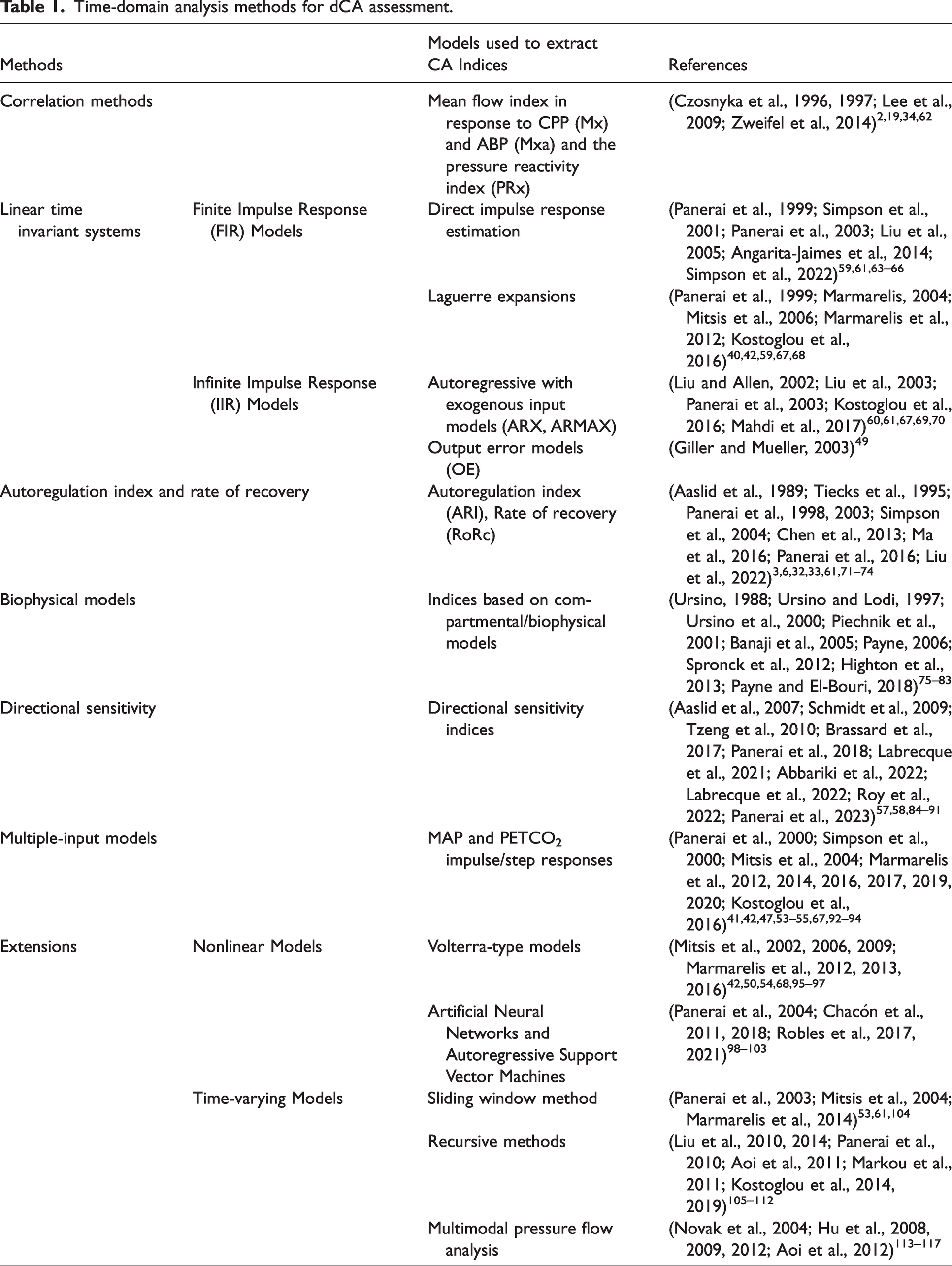
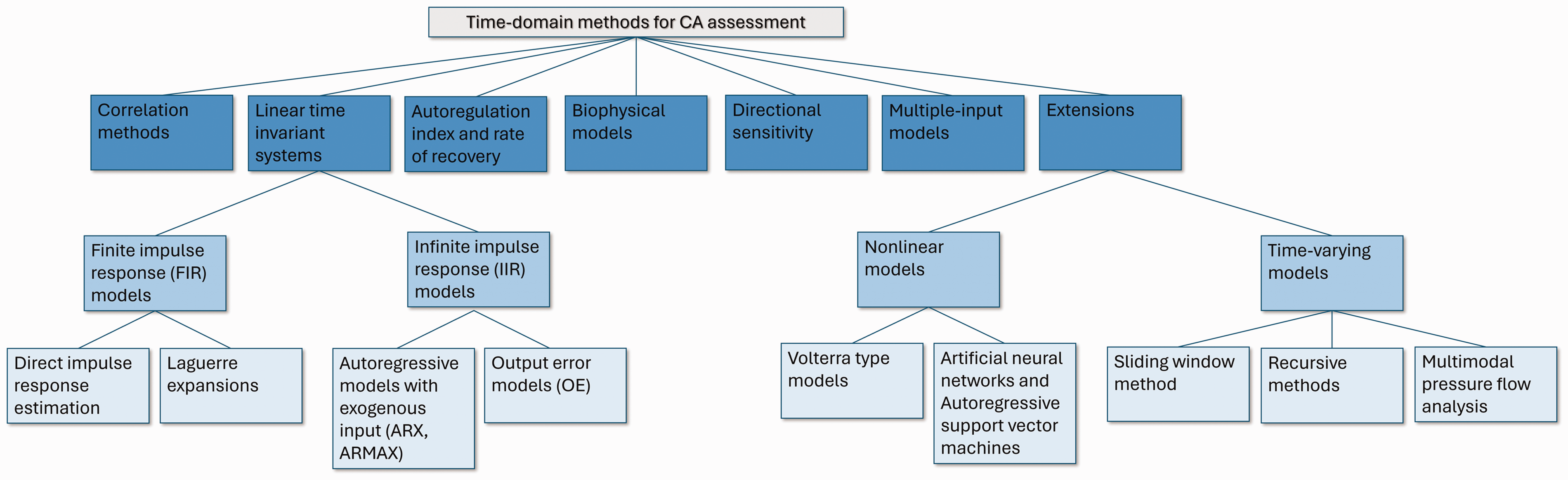
Overview of time-domain approaches for evaluating dCA.

Methods

Correlation methods

In the simplest case, the CBv (or NIRS-derived signals such as cerebral oxygenation or hemoglobin volume) can be expressed at each time point as a linear function of CPP or ABP at the same time.^2,19

$$y\left(n\right)=bx\left(n\right)+\epsilon \left(n\right)$$

(1)

where $y\left(n\right),x\left(n\right)$ are CBv and CPP or ABP signals (after subtracting their average value) at time point $n$ , respectively, and $\epsilon \left(n\right)$ is assumed to be additive noise (e.g., measurement noise or unobservable/unmodeled factors). The coefficient $b$ describes the relationship between input and output. If $b>0$ , the relationship between CBv and CPP or ABP is positive, whereas if $b<0$ the relationship is negative. $b$ can be estimated by minimizing the sum of the squared residuals of the linear regression model of equation (1). Pearson’s correlation coefficient is a rescaled version of $b$ , ranging between −1 and 1. In CA, the correlation coefficient between CPP and CBv is referred to as the Mean Flow Index in response to CPP (Mx) and the correlation between ABP and CBv as the Mean Flow Index in response to ABP (Mxa). On the other hand, the Pressure Reactivity Index (PRx) is defined as the correlation between ABP and ICP. Mx, Mxa and PRx are usually estimated in consecutive windows of the data (see below).

Based on Lassen’s curve, the relationship between CBv and ABP (or CPP) is non-linear. The correlation method (equation (1)), however, uses the linearization principle around the current static working point. Below the lower limit and above the upper limit of autoregulation, the correlation between CBF and ABP (CPP) should be positive (theoretically around +1, as the system is linear outside the autoregulation limits). Within the autoregulation range, the correlation is expected to be closer to zero or negative,^2,118 depending on the exact shape of the Lassen curve, which may show negative slope close to but above the lower limit of autoregulation, particularly in patients slightly hyperventilated.^118,119

For TCD signals, the coefficient $b$ of equation (1) represents the inverse of cerebrovascular resistance (CVR; per unit of cross-sectional area of the investigated artery), which is linearly dependent on CPP between the lower and upper limits of autoregulation, maintaining CBv approximately constant. For NIRS signals, the interpretation of $b$ is less obvious. It depends on CVR, but also on hematocrit, cerebral metabolic rate of oxygen and oxygen diffusivity.

For ICP-derived cerebrovascular reactivity parameters such as PRx, ² the relationship between $x$ and $y\mathrm{ }$ is more complex. The coefficient $b$ describes jointly the change in arterial cerebral blood volume evoked by a change in CPP or ABP, and the change in ICP-controlled cerebrospinal pressure-volume curve.

Correlation indices have been developed following some simplified assumptions, with an intention to use them in long-term monitoring of relative changes in CA within the period of critical care (days/weeks) or surgical intervention (3–6 hours). These indices are typically calculated as follows:

All signals are band-pass filtered between 0.005 and 0.05 Hz. It is important that the energy of the signals above 0.05 Hz should be minimized to avoid influence of components containing very little information about CA (i.e., respiratory waves and pulse waveform).

10 second time averages of CPP or ABP and CBV, NIRS-derived or ICP values are continuously calculated, and updated every 10 seconds.

30 consecutive samples from the previously calculated averages are taken to compute correlation coefficients.

Operations 2 and 3 are repeated within sliding windows, depending on the requirements of the monitoring system (in clinical practice, a 1-minute shift is usually used ¹²⁰ )

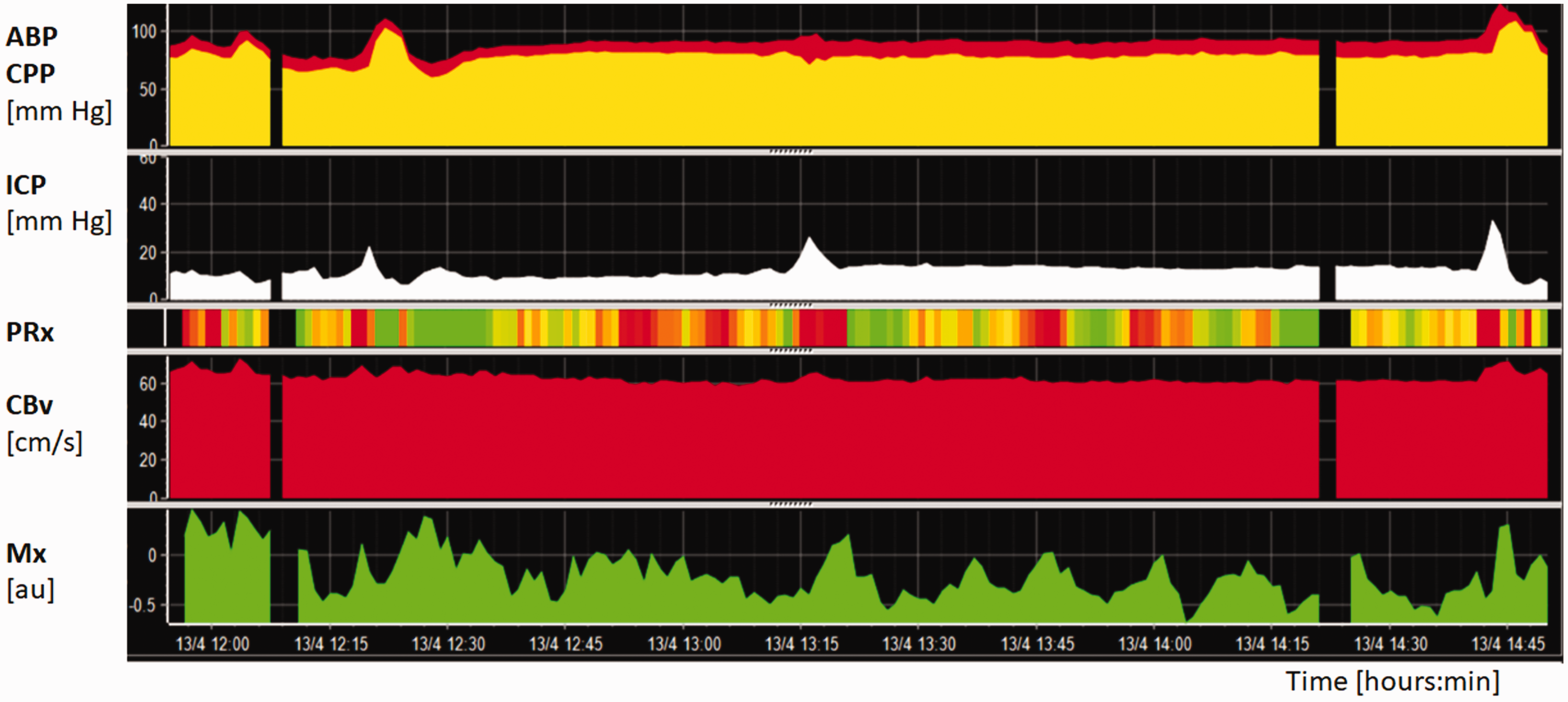
The resulting autoregulation indices are displayed along with other parameters derived from multimodal brain monitoring. All these time trends describe jointly complex brain physiology (Figure 2).

Figure 2.

Example of a three-hour monitoring period of autoregulation in patients suffering from traumatic brain injury. ABP and CPP are shown in the upper panel, whereas ICP in the second horizontal panel. CBv in the left MCA (fourth horizontal panel), measured with TCD, was overall stable (defined as FVl). dCA was monitored using Mx (bottom panel) and PRx (third horizontal panel), which are represented using a color code where green and red indicate normal and altered pressure reactivity, respectively. The graph shows that in spite of the low ICP, CA is continuously fluctuating.

Recommendations:

For the raw data, before bandpass filtering, a minimum sampling rate of 20 Hz is recommended.^{19,118,121,122} Lower sampling frequencies are generally not employed in most of the bed-side monitoring systems, as ICP is typically part of a multimodal set-up.

In general, no additional pre-processing besides band-pass filtering is necessary, as the 10-second moving average smooths out the employed signals.

Spikes (e.g., collecting/flushing blood samples from the arterial line) may be corrected automatically using as a criterion the presence of undisturbed blood pressure pulses. Alternatively, more sophisticated methods can also be employed. ¹²³

The use of a correlation threshold is not necessary since information on CA state can be deduced by high correlation values (indicating impaired CA) and low correlation values (around zero or negative, indicating preserved CA). However, threshold for PRx of 0.30 can be adopted from experimental studies by direct comparison to the lower limit of autoregulation of Lassen curve ¹⁰ or 0.25 for Mx (based on the analysis of the mortality rate of a large cohort of patients after traumatic brain injury ¹²⁴ )

The possibility of using TCD for long-term CA monitoring is limited, as contemporary probe holders cannot prevent change of probe position in situations such as patient turning, physiotherapy and other maneuvers. Specialized ‘robotic’ probe holders are not yet widespread and are far from being ideal for long-term TCD monitoring. ICP pressure reactivity indices and NIRS-based methods are ideally crafted for long-term monitoring.

An important clinical application of continuously recorded autoregulation indices is monitoring of the so-called ‘optimal’ CPP and ABP. Optimal CPP and ABP are pressure levels which indicate the middle point of Lassen’s curve (between the lower and upper limits of autoregulation). In continuous brain monitoring following traumatic brain injury, the optimal CPP level can be used as a target management level to help prevent secondary brain injury. ¹²⁰ In cardiac surgery, optimization of ABP helps in avoiding post-operative delirium and acute kidney injury. ⁷⁴

Linear Time Invariant systems

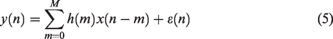
dCA can be modeled as an LTI causal system, whereby ABP or CPP is the input and CBv the output. In the time domain, the dynamic relationship between the input 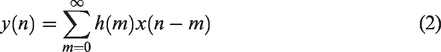$x\left(n\right)$ and output $y\left(n\right)$ can be fully described by the system impulse response $h\left(m\right)$ , ( $n$ and $m$ are discrete time-indices, with $n$ denoting the present time and $m$ representing the lag of past values)

$$y\left(n\right)=\sum _{m=0}^{\mathrm{\infty }}h\left(m\right)x\left(n-m\right)$$

(2)

where $h\left(m\right)$ is a function that weights the input past and present values ( $x\left(n-m\right)$ ) to generate the output present value ( $y\left(n\right)$ ) and describes the causal effects of ABP or CPP on CBv.

In the frequency domain, the convolution operation of equation (2) becomes,

$$Y\left(\omega \right)=H\left(\omega \right)X\left(\omega \right)$$

(3)

where $X\left(\omega \right)$ and $Y\left(\omega \right)$ are the discrete Fourier Transforms of the input and output, respectively, $\omega$ is frequency and $H\left(\omega \right)$ is the system frequency response, which is equal to the Fourier transform of the impulse response $h\left(m\right)$ . This quantity is estimated when using TFA as follows,

$$H\left(\omega \right)=\frac{S_{xy}\left(\omega \right)}{S_{xx}\left(\omega \right)}$$

(4)

where $S_{xy}\left(\omega \right)$ is the cross-spectrum between ABP and CBv and $S_{xx}\left(\omega \right)$ is the auto-spectrum of ABP.^18,26,125 Note that, strictly, the frequency response, which is obtained using TFA, is formally defined as the transfer function for $s=j\omega$ .

In the case of time-domain methods, the main objective is the accurate estimation of the impulse response $h\left(m\right)$ , either directly or based on some estimated model coefficients. In the dCA literature, the most widely used approaches have been finite impulse response (FIR) and infinite impulse response (IIR) models, which we cover in the following subsections. Note that, similar to recommendation #5 in, ²⁶ the input and output data are assumed to be mean beat-to-beat ABP (MAP) and CBv signals. Based on recommendation #7 in, ²⁶ beat-to-beat data should be linearly interpolated to obtain equidistant time intervals.

Finite impulse response (FIR) models

Equation (2) can be implemented as an FIR model, ⁴³ assuming that the impulse response of the system has a finite duration such that the sum is of finite, rather than infinite length. In this case, the CBv signal can be expressed as a weighted linear combination of a finite number of present and past MAP values, ⁶⁴

$$y\left(n\right)=\sum _{m=0}^{M}h\left(m\right)x\left(n-m\right)+\epsilon \left(n\right)$$

(5)

where $M$ (the system memory or model order) is the length (duration) of the impulse response $h\left(m\right)$ . The error term $\epsilon \left(n\right)$ includes the effects of measurement noise, as well as the effect of additional physiological variables (other than ABP or CPP) on the measured CBv signal.

Direct impulse response estimation

The basic idea of estimating the impulse response is to find $h\left(m\right)$ from the recorded MAP $x\left(n\right)$ and CBv $y\left(n\right)$ , such that the measurement noise/unobservable factors $\epsilon \left(n\right)$ are of small amplitude and unrelated to the effects of MAP. Typically, the mean-square value of $\epsilon \left(n\right)$ , calculated over the duration of the recording, is minimized, which leads to the so-called Wiener solution ¹²⁶ expressed using the following estimator for $h\left(m\right)$ :

$$\widehat{\mathit{h}}={\mathit{R}}_{xx}^{-1}{\mathit{r}}_{xy}$$

(6)

where ${\mathit{R}}_{xx}$ and ${\mathit{r}}_{xy}$ are the auto-correlation matrix of $\mathit{x}$ and the cross-correlation vector between $x$ and $y$ , respectively; $\widehat{\mathit{h}}$ is the vector of $h\left(m\right)$ , for all values of $m$ . Alternatively, the least squares estimate based on the Moore-Penrose pseudoinverse for finite data lengths can also be used for impulse response estimation. This approach is described in further detail in the Supplementary Material (section I. 1.1). The aforementioned procedure aims to ‘explain’ as much of $y$ from $x$ as possible through this mathematical relationship, regardless of specific physiological mechanisms. Therefore, $h\left(m\right)$ should not be interpreted as reflecting only the direct causative effect of ABP on CBv fluctuations. Additionally, non-linear interactions may mean that more of the variability in $y$ could potentially be explained from $x$ , with more complex mathematical models. Once the impulse response has been estimated, the challenge becomes to quantify autoregulation from it.

A common approach is to find the step response, which may be more straightforward to interpret physiologically, compared to the impulse response. The step response can also be directly compared to the ten ARI template step responses proposed by Tiecks et al. ³² (see also section Autoregulation index and Rate of Recovery below), gauging dCA from completely absent to efficiently functioning. The step response can be readily calculated as the cumulative sum of the impulse response:

$$s\left[n\right]=\sum _{m=0}^{M}h\left[m\right]$$

(7)

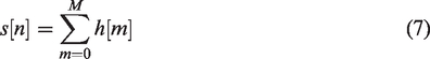
The step response of equation (7) shows how CBv changes in response to a step change in MAP: a near complete and fast return to baseline would reflect functioning dCA, whereas a passive CBv step response following the MAP change would suggest impaired dCA. Even though this information is also contained in the impulse response, the step response is more directly interpretable; hence it has been used more frequently in dCA studies.^63,65,72,127

Time-domain metrics that reflect the speed of recovery, such as the ARI and RoRc (section Autoregulation index and Rate of Recovery), can be subsequently derived from the step response. Both metrics have been recommended in the recently updated consensus White Paper of Panerai et al. ²⁶ (recommendation #18 in ²⁶ ) Specifically, RoRc was initially proposed to evaluate dCA in patients with Moyamoya disease at different stages. ³³ It has been subsequently tested against a number of autoregulatory metrics and shown to be statistically more reliable than phase, coherence or ARI in terms of inter-subject variability. ⁶⁵

The Fourier Transform of the impulse response yields the frequency response (equation (4)) and therefore provides an alternative to TFA. Frequency domain parameters such as phase and gain, as used in TFA analysis^18,26 can thus again be obtained. The results can be expected to be similar, but not identical to those obtained from TFA, especially for higher frequencies (>0.15 Hz) where the Signal-to-Noise ratio (SNR) is lower. Furthermore, FIR models are causal (i.e., the impulse response is zero for negative time) and time-limited (by the chosen order of the FIR filter), whereas TFA-based methods are less constrained. An example of step, gain, and phase responses derived from a FIR model can be found in ³³ (Figure 1 in ³³ ).

Previous studies^61,64 reported tenth-order ( $M=10)$ and sixth-order ( $M=6)$ impulse responses, respectively, to describe the dynamics of dCA at a 1 Hz sampling rate. However, further investigations on the selection of the model order are still required. In early work using FIR filters, ⁶³ a first-order model ( $M=1)$ was employed (i.e., a FIR filter with only two parameters). This can yield the simplest form of a high-pass filter (a key feature of active dCA) described by a first-order difference equation, and dCA can be quantified directly from the two filter parameters. One of the main advantages of this formulation is that dCA can be estimated from very short segments of recordings (i.e., 40–60 seconds); however, it is unlikely that such a simple model can provide an accurate representation of the more complex and longer duration dCA responses.

In summary, FIR modeling is closely related to TFA analysis, with the main difference being that the impulse responses are assumed to be finite and causal (which seems a reasonable assumption for assessing the effect of MAP changes on CBv). There are many options on how to quantify dCA from the estimated impulse responses, including those based on the frequency domain (gain and phase) or step responses (e.g., ARI or RoRc).

Recommendations:

Although there is little published evidence, theoretical considerations suggest that most of the recommendations in ²⁶ can be applied to FIR model time-domain estimation. For example, the recommendations #1–9 in ²⁶ for data pre-processing are applicable to obtaining FIR models.

The impulse response can be estimated using the mean-square error estimator of equation (6) or the least-squares estimate described in the Supplementary Material (section I. 1.1). When calculating the required auto- and cross-correlation functions, we suggest using a biased estimator to improve the reliability, given the relatively short length of data recordings.

Typical model orders are expected to be between 5 to 15 lags for a 1 Hz sampling rate, corresponding to a 5 to 15 seconds memory in the effects of MAP on CBv. ⁶⁶

To improve calculation of the inverse of the autocorrelation matrix of equation (6) or the pseudoinverse required for least squares estimation (which may become problematic when the original matrices are ill-conditioned, with some eigenvalues being very close to zero), regularization techniques can be applied (see Supplementary Material, section II. 1.3). These include ridge regularization or regularization with constraint on the size of the change in the model coefficients, since the impulse response weights are expected to change in a smooth manner and progressively decrease with increasing time lag. ¹²⁸

Laguerre expansions

An alternative way of estimating the impulse response function of an LTI system (equation (5)), which is robust in low SNR environments, is the Laguerre expansion technique (LET), whereby the impulse response function is expanded in terms of the orthonormal basis of discrete-time Laguerre functions (DLFs).^39,40 LET was originally introduced for the robust estimation of nonlinear time-invariant (and possibly multivariate) input-output models based on a hierarchy of convolutional functionals (Volterra functionals) of finite order. Here, we will discuss the first-order case (LTI models) with single input and output in the context of dCA studies, where the input is MAP, and the output is CBv.

Before we proceed with the specific steps for the estimation of the impulse response $\mathit{h}\left(\mathit{m}\right)$ using LET, we clarify the rationale of this approach and the underlying assumptions for its proper application.

We employ the canonical model form of equation (5), because it is universally applicable to all LTI systems, thus avoiding potential pitfalls of ad hoc modeling schemes. This is premised on the assumption that nonlinearities and time variations of the underlying true system remain negligible for the range of normal spontaneous variations and the employed data length. Extensions to nonlinear and/or time-varying systems are feasible (see section Extensions).

The model residual term $\epsilon \left(n\right)$ contains the effects upon CBv of several unobservable confounders (e.g., variations of blood CO2 tension and blood oxygen saturation, respiration, endocrine and metabolic effects etc.) and of measurement noise at a combined SNR level of 0–5 dB. This is suggested by previous studies using one and two-input LET models to model dCA, which have reported average normalized mean-square errors (NMSEs) between 40 and 50%.^{41,53 –55,93,94} Since the length of the data records is usually 5–10 min in practice, the task of reliable estimation of the impulse response function/kernel requires a robust estimation method (such as LET).

It is assumed that a satisfactory approximation of the true impulse response can be obtained with a relatively small number of DLFs (<8).

DLFs have a built-in exponential term that makes them suitable for approximating the dynamics of physical systems that decline exponentially (in absolute value) after a certain finite lag value. The rate at which the DLFs asymptotically decline is defined by the discrete Laguerre parameter ‘alpha’, which lies between 0 and 1, and chosen according to the characteristics of the system of interest (see also Supplementary Material I 1.2).

The impulse response 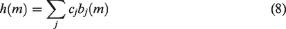$\mathit{h}\left(\mathit{m}\right)$ can be expanded as a linear combination of DLFs { $b_j\}$ (see Supplementary Material, section I. 1.2) as:

$$h\left(m\right)=\sum _j{c}_j{b}_j\left(m\right)$$

(8)

where { $c_j$ } are the Laguerre expansion coefficients that are estimated from the data via linear regression according to equation (9). The summation over $j$ includes all DLFs needed for the impulse response expansion using the selected parameter ‘alpha’, as determined through a search procedure that minimizes the Bayesian Information Criterion (BIC) ¹²⁹ (see Supplementary Material, section II. 2.1). The BIC is a model order selection criterion that can be used instead of cross-validation when the data length is relatively short. It essentially balances the total number of data points and number of model coefficients against the accuracy of the model fit. The Laguerre expansion of equation (8) transforms the input-output relation of equation (5) into equation (9), where the time-series { $v_j\left(n\right)$ } are convolutions of the MAP input with the DLFs (see Supplementary Material, section I. 1.2):

$$y\left(n\right)=\sum _j{c}_j{v}_j\left(n\right)+\mathrm{ }\epsilon \left(n\right)$$

(9)

Equation (9) involves linearly the unknown Laguerre expansion coefficients that can be estimated via linear regression and least squares estimation, ³⁹ which yields optimal estimates for Gaussian residuals. Following estimation of the expansion coefficients, the impulse response estimates can be constructed using equation (8) and the model prediction for any given input can be computed using equation (5). This approach has found successful application in several studies of dCA to date.^{41,42,50,53 –55,68,93,94} Some of these studies have also taken the effects of contemporaneous PETCO₂ variations upon CBv into account (see sections Multiple-input Models and Extensions).

An illustrative example of the LET for dCA assessment in the case of a two-input model (MAP and CO₂) is given in section Multiple-input Models (Figure 6).

Recommendations:

The input-output beat-to-beat data should be preprocessed to subtract the mean value (demeaning) and remove possible outliers by applying hard-clipping at +/− 2.5 standard deviations. To make the input-output data evenly sampled, the computed MAP and CBv values for each beat should be placed at the midpoint of the respective R-R interval and are evenly resampled every 0.5 seconds (sampling frequency of 2 Hz) via cubic-spline interpolation.^54,55,93,94 High-pass filtering above 0.005 Hz is also recommended to remove very low frequencies or slow trends from the input-output data.

The optimal number L of DLFs and their alpha parameter ought to be determined through a two-dimensional search procedure over a grid of values for $L$ ranging from 1 to 8 and alpha ranging from 0.1 to 0.9 using a step of 0.1 or smaller, which seeks to minimize the BIC (see Supplementary Material, section II. 2.1). When a cohort is examined, it is recommended that these optimal values ought to be the averages of individual searches minimizing the BIC for each subject in the cohort,^54,55,93,94 and should be clearly reported.

Infinite Impulse Response (IIR) models

Expressing the output variable (CBv) as a function of one or more of its past samples, in addition to the present and past samples of the input (MAP), yields an impulse response of infinite duration (IIR model). The main advantage of IIR models in comparison with FIR models is that they typically result in a lower number of unknown parameters.

Autoregressive models with exogenous input (ARX)

An ARX model of order ( $n_a$ , $n_b$ ) is an extension of the FIR model that also contains previous output values: ⁴³

$$y\left(n\right)=\sum _{m=1}^{n_a}{a}_{m}y(n-m)+\sum _{m=0}^{n_b}{\beta }_{m}x(n-m)+\epsilon \left(n\right)$$

(10)

where the output $y\left(n\right)$ is CBv, the exogenous input $x\left(n\right)$ is MAP, and the autoregressive component $y(n-m)$ refers to the CBv history that is included.^{49,60,61,67,69,70,130,131} As in the FIR case, the ARX model is linear in the parameters and the coefficients { $a_m$ } and { ${\beta }_m$ } can be estimated by a closed-form least squares solution. It can also be extended to multiple exogenous inputs to take into account the effect of other physiological variables on dCA (see section Multiple-input Models). For more details regarding ARX model estimation please see the Supplementary Material (section I. 2 and section II).

An important aspect related to ARX modeling is the selection of appropriate values for ( $n_a$ , $n_b$ ). Selecting a model with higher values of ( $n_a$ , $n_b$ ) than needed may result in overfitting, i.e., capturing the relationship between the input and output training data very accurately but failing to replicate it on unseen data. This implies that the model is describing transient/spurious effects from unobservable variables or noise sources that do not reflect the mechanisms of interest. Previous dCA studies have reported model orders $n_a$ equal to 1 or 2 and $n_b$ between 1 and 5^60,61,69,70 for sampling rates of 1 and 10 Hz. A wider range of model orders ( $n_a$ and $n_b$ between 1 and 10) were considered in.^49,67,132 It is common practice to select predefined model orders based on the literature, however, below we stress the importance of applying appropriate model order selection techniques for a dataset of interest (see also Supplementary Material, section II. 1).

Recommendations:

No filtering should be applied to the data. ARX models perform best on the broadband beat-to-beat signals. DC offsets and linear trends should be removed prior to ARX modeling to reduce the amount of the very low-frequency power (Recommendations #8 and #9 in ²⁶ )

The values of ( $n_a$ , $n_b$ ) should be selected using cross-validation,^68,133 in case a sufficient amount of validation data is available, or model order selection criteria such as the Akaike Information Criterion (AIC) ¹³⁴ or Bayesian Information Criterion (BIC), ¹²⁹ when this is not the case. Cross-validation involves segmenting the data into training and testing sets. The ARX model coefficients are estimated for increasing model order values on the training set, and the identified model is applied to the testing set. The model orders that achieve the lowest NMSE between actual and predicted output on the testing set are selected (Supplementary Material, section II. 1.1). On the other hand, model order selection criteria account for the increase in the model complexity along with the prediction error^{50,53,61,67,105,130} (Supplementary Material, section II. 1.2). The optimal model is found when the additional penalty for using extra coefficients exceeds the added benefit in terms of reducing the NMSE. In the Supplementary Material (section II), we further discuss model order selection.

Caution should be exercised with regards to the sampling rate of the data. Apart from the fact that oversampling increases the number of data points to be processed, it may lead to numerical issues^135,136 (low condition number values for the regression matrix ¹³⁷ ) and suboptimal results especially in the low frequency range. ⁴³ This occurs for any system identification method that uses the one-step ahead prediction error as a cost function.^43,136,138 If the sampling rate is high, the variation in the data from one point to the next may be very small, resulting in near perfect one-step ahead prediction even for very few past lags. This also poses problems in terms of model order selection, leading to model structures that may under-represent the true underlying dynamics. Recommended sampling rates are between 1 Hz and 5 Hz for mean beat-to-beat MAP and CBv signals. Another way to mitigate the effects of oversampling is the use of the ARX multi-step or infinite-step ahead prediction error as cost function, ⁶⁷ as it may result in a better approximation of the underlying dCA dynamics (see also section Output-Error models^49,139)

As the resulting model orders may depend on the sampling rate, it is recommended that the sampling rate and the final selected orders are clearly reported.

An extension of the ARX model is the ARMAX structure. In the ARX technique the noise enters the model in a very restricted way (i.e., the deterministic and stochastic ARX part share the same dynamics, which may not be realistic in some cases). An ARMAX model provides greater flexibility by modeling the noise component as a moving average (MA) white noise process. An ARMAX ( $n_a$ , $n_b,n_c)$ model can be expressed as follows:

$$y\left(n\right)=\sum _{m=1}^{n_a}{a}_{m}y(n-m)+\sum _{m=0}^{n_b}{b}_{m}x(n-m)+\sum _{m=1}^{n_c}{c}_m\epsilon (n-m)+\epsilon \left(n\right)$$

(11)

Equation (11) assumes that the underlying noise that drives the system is colored (non-white), i.e., it exhibits some structure. Note that in the dCA literature, ARX models are often referred to as ARMA models (where AR represents the CBv feedback and MA the linear combination of current and past MAP values). However, in the system identification literature, the MA term usually refers to the noise characteristics. ⁴³ Therefore, the distinction between ARX and ARMAX relies solely on the assumptions that are made regarding the driving noise component.

In contrast to the ARX approach, ARMAX identification results in a nonlinear optimization problem because the product of the unknown coefficients ${\{c}_k\}$ and the noise process $\epsilon \left(n\right)$ enter into the cost function. Numerical methods for nonlinear optimization are iterative. Some examples include the Newton-Gauss and Newton-Raphson algorithms. Recursive methods such as the recursive pseudo-linear least squares and prediction error methods can also be used for ARMAX estimation. ¹⁴⁰ Due to their computational complexity, ARMAX models have not been used for dCA analysis. However, ARMAX models would be suitable for modeling dCA, as the noise characteristics are expected to exhibit some structure, particularly in the case of one-input models, where the effect of additional physiological variables (e.g., PETCO₂) is not taken into account.

In Figure 3 we present ARX and ARMAX analysis results for a representative segment of 5 min MAP-CBv experimental recordings during resting conditions. The data was detrended and resampled at 1 Hz for computational efficiency. Model orders were selected based on a two-fold cross-validation scheme, whereby the first 50% of the data was used for training and the rest 50% for testing and vice versa. For the ARX model, the optimal order was found to be ( $n_a$ , $n_b)=(2\text{,}4)$ (similar values were also obtained in ⁸⁶ ) whereas for the ARMAX model the optimal order was ( $n_a$ , $n_b,\mathrm{ }{n}_c)=(2\text{,} 3,2)$ . Figure 3(a) and (b) depict the estimated impulse responses, as well as the CA gain (cm/s/mmHg) and phase (rad) functions for both models (blue ARX; red ARMAX). Figure 3(b) is essentially the magnitude and the phase of the discrete Fourier Transform of the impulse responses of Figure 3(a). As expected, dCA exhibits high-pass characteristics. The BIC scores suggested that the ARMAX model resulted in a better overall fit. Slight differences in the very low (<0.07 Hz) and high (>0.2 Hz) frequency ranges can be observed in the frequency responses obtained by the two methods. These differences could be more significant under different experimental conditions and noise levels. Since the ARMAX model takes into account the structure of the noise (which could be either measurement noise or unobservable factors), it may provide less biased dCA estimates compared to the ARX model. We therefore encourage researchers to compare further these two approaches.

Figure 3.

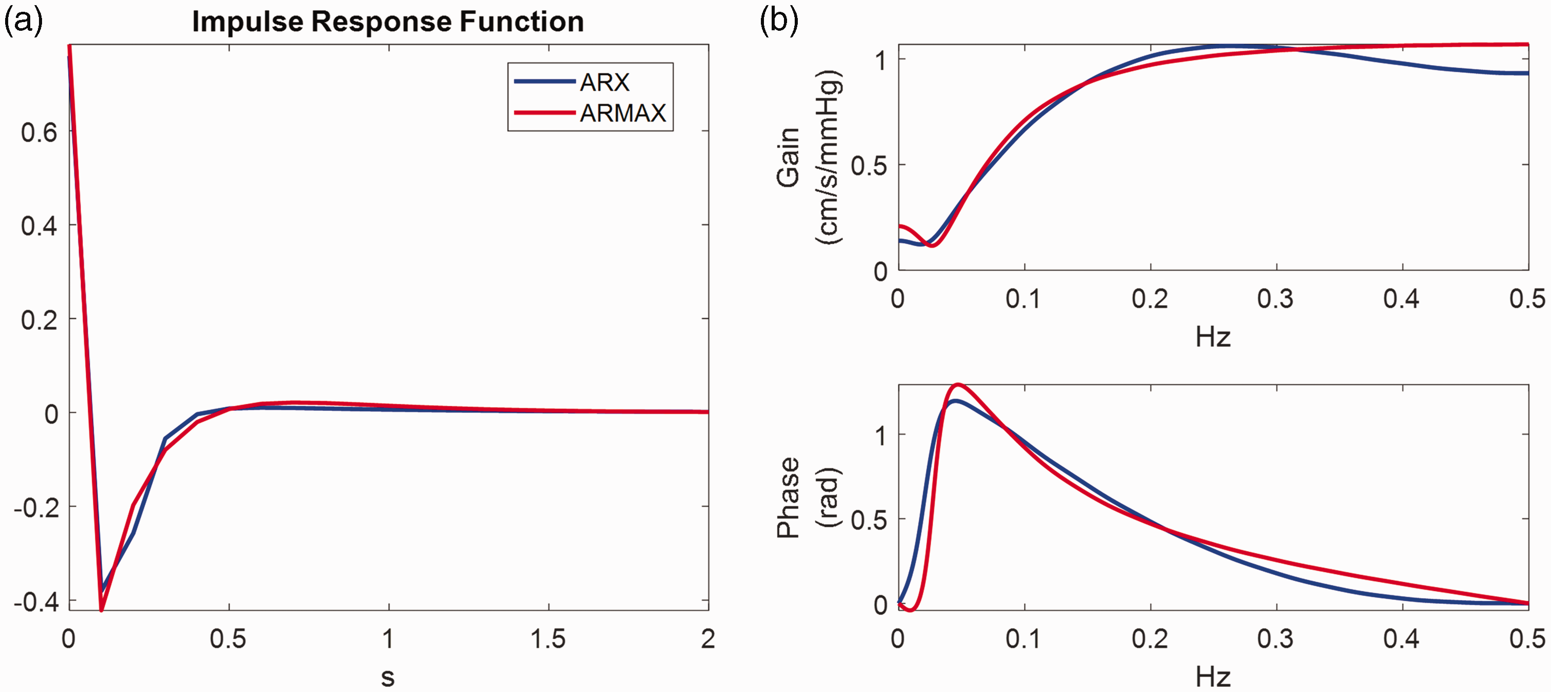
ARX vs ARMAX analysis for a representative set of 5 min experimental resting MAP-CBv recordings resampled at 1 Hz. (a) The estimated impulse responses in the time and (b) the frequency domain (blue ARX; red ARMAX). The top and bottom subplots of (b) depict the gain (cm/s/mmHg) and phase as a function of frequency. We applied a 2-fold cross-validation scheme, whereby the first 50% of the data is used for training and the rest 50% for testing and vice versa. The minimum NMSE was achieved using ARX model orders with ( $n_a$ , $n_b)=(2\text{,}4)$ and ARMAX models orders with ( $n_a$ , $n_b,n_c)=(2,3,2)$ .

Output-error models (OE)

The OE model is a specific formulation of the IIR model. It consists of a transfer function that relates the measured input to the output and includes additive white noise. An OE model of order (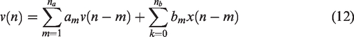 $n_a$ , $n_b)$ can be expressed in the time domain as follows, ⁴³

$$v\left(n\right)=\sum _{m=1}^{n_a}{a}_{m}v(n-m)+\sum _{k=0}^{n_b}{b}_{m}x(n-m)$$

(12)

$$y\left(n\right)=v\left(n\right)+\epsilon \left(n\right)$$

(13)

where $v\left(n\right)$ is an auxiliary signal, $y\left(n\right)$ and $x\left(n\right)$ are the observed output (CBv) and input (MAP) respectively, and $\epsilon \left(n\right)$ is additive noise. In contrast to the ARX model, where the noise is modulated by the system dynamics before generating the output, in the OE model, the noise is defined as the difference between observed and predicted output. The identification method typically used for OE models is the prediction error method (similar to ARMAX models).

Giller et al. ⁴⁹ was the first study in which OE models were employed for dCA analysis in combination with spontaneous MAP oscillations. They used a sampling frequency of 0.5 Hz and tested OE models of orders up to 20 based on a two-fold cross-validation procedure. A fit of 25% on the output variation of the testing data was set as a threshold. 4th and 6th order models (i.e., $n_a=n_b=\left\{4\text{,}6\right\}$ ) were selected as optimal. As in the ARX/ARMAX case, model order selection is crucial for accurate impulse response estimation. The recommendations of ARX/ARMAX models apply to OE models as well.

Autoregulation index and rate of recovery

Autoregulation index (ARI)

The ARI model assumes that the CBv response to changes in MAP can be described by a second order difference equation. ³² While not explicitly based on biophysical laws, the ARI model assumes a specific structure. It can be applied either to resting state fluctuations or to large, induced, fluctuations such as the thigh cuff test. The equations are based on three parameters: gain, $K$ ; damping factor, $D$ ; and time constant, $T$ :

$$dP=\frac{\left(\mathit{MAP}-\mathit{cABP}\right)}{\left(\mathit{cABP}-\mathit{CrCP}\right)}$$

(14)

$$x_2\left(n\right)=x_2\left(n-1\right)+\frac{x_1\left(n\right)-2D{x}_2\left(n-1\right)}{fT}$$

(15)

$$x_1\left(n\right)=x_1\left(n-1\right)+\frac{dP\left(n\right)-x_2\left(n-1\right)}{fT}$$

(16)

$$y\left(n\right)=1+dP\left(n\right)-K{x}_2\left(n\right)$$

(17)

where $y\left(n\right)$ corresponds to CBv, $dP\left(n\right)$ is the normalized change in MAP, relative to its control value, cABP. CrCP is the critical closing pressure, usually assumed to be constant at 12 mmHg. The sampling frequency is denoted by $f$ and the state variables, $x_1\left(n\right)$ and $x_2\left(n\right)$ , are assumed to be equal to zero in the control phase. Note that the ARI representation may be also viewed as an ARX model. ¹¹² The ARI is a metric that varies between zero (no autoregulation) and 9 (maximal autoregulation) and corresponds to ten different sets of the values of $K$ , $D$ and $T$ in the above model. For each value of ARI, or combination of $K$ , $D$ and $T$ values, the corresponding $y\left(n\right)$ ‘step response curve’ quantifies the temporal pattern of the CBv signal resulting from a hypothetical step change in MAP. ³²

Although numerical implementation of equations (14) to (17) is relatively straightforward for sampling frequencies within the range [4–10] Hz, standardization is lacking for several aspects of the estimation process and limited evidence is available about the relative reliability of different options. The majority of studies have adopted the original conversion table proposed by Tiecks et al. ³² to translate values of $K$ , $D$ and $T$ into a single value of ARI, but alternatives have also been suggested, ¹⁴¹ including the use of a model-free ARI. The most contentious aspect of ARI calculation is the optimization of the model error, leading to a choice of one of the 10 possible values of ARI. Specifically, the model prediction error is often expressed as the MSE of the difference between the estimated output $y\left(n\right)$ and measured values of CBv. The main problem with this approach is that, due to the presence of noise in measurements of MAP and CBv, the MSE may not exhibit a clear minimum value, thus leading to erroneous ARI estimates. ⁷¹

This problem can be overcome by matching the ARI-based step response curves to the CBv step responses calculated by TFA or ARX models.^22,61 Calculation of the CBv step response can be obtained by TFA ²⁶ or using an ARX/ARMAX structure as described above. In addition to its reduced sensitivity to noise, this approach for calculation of the ARI has some additional advantages. First, it allows visual inspection of the CBv temporal pattern, followed by rejection of responses that are not physiologically plausible.^73,142 Specifically, CBv step responses are not considered physiologically plausible if a sudden change in ABP does not lead to a corresponding marked change in CBv, or if the response is continuously rising in a ramp-like fashion, or followed by a negative tail that is much larger in absolute value when compared to the initial jump in CBv. Second, the step response approach is not sensitive to amplitude changes, thus not requiring any previous normalization of CBv and MAP as needed for the equations above, or any pre-set values of CrCP. ³² Given these considerations, the need for greater standardization, and the evidence available, the following recommendations apply to the estimation of the ARI.

Recommendations:

Calculation of the Tiecks standard step response curves should be based on the values of $K$ , $D$ and $T$ as originally proposed in. ³²

Model estimated CBv step responses obtained from measured data can be obtained via different time-domain models (section Linear Time Invariant systems) or TFA.

Visual inspection of CBv step responses is essential for removing responses that are not physiologically plausible.

Estimation of the ARI should be made by minimizing the normalised MSE between the data predicted CBv step response and the Tiecks curve leading to the best fitting.

Non-integer values of ARI can be obtained by interpolation of the original 10 curves provided by the Tiecks model. ³² One possible approach is to perform cubic spline interpolation for the original $K$ - $D$ - $T$ table proposed by Tiecks et al., ³² followed by resampling it 100x, thus leading to 1000 combination of ARI values, corresponding to estimates with two decimal digits.

Rate of recovery (RoRc)

The RoRc has been adopted in several clinical studies and shown to be sensitive to deterioration of dCA in stroke and other cerebrovascular conditions.^{3,33,74,143 –146} Recommendations for its calculation should follow the same steps above for the calculation of the ARI, up to the estimation of the CBv step response and its visual inspection. Once a physiologically plausible CBv step response has been obtained, the RoRc can be obtained by the ratio $\frac{\Delta \mathrm{CBv}}{\Delta T}\mathrm{\hspace{0.17em}\times \hspace{0.17em}}100\%$ , where $\Delta \mathrm{CBv}$ is the drop of CBv from its maximum value after $\Delta T=3$  s into the response. Given that the RoRc is obtained by a ratio, it may be reasonable to expect that it may be more sensitive to noise than the ARI; however, further comparative studies are needed to assess the agreement and sensitivity to noise of these two indices.

Biophysical models

Biophysical models of dCA vary from simple, high-level, models to highly detailed descriptions of the underlying mechanical and physiological processes that govern dCA.^{76,79 –82,147 –150} The first whole-brain dCA model was proposed by Ursino ⁷⁵ based on equivalent electrical circuit concepts. It was the first model to suggest that changes in arterial conductance govern the autoregulatory response. This model has been very influential and most subsequent biophysical models that have been proposed are linked to it (see for example^{76 –80,149}) although the complexity of the feedback mechanisms varies significantly between studies. Simpler models are more amenable to estimating their parameters from experimental data, whereas more complex models aim to provide greater insight into the underlying physiological processes.

Relatively few studies have attempted to estimate model parameters from these compartmental models. The early study by Ursino et al. ⁸¹ estimated four parameters from time-series data recorded in 20 severe acute brain damage patients using a least-squares approach; Lodi et al. ¹⁵¹ then used similar data, with the addition of ICP, in a study cohort of six patients with severe head injury; Ursino et al. ⁸³ used data collected from 13 severe head injury patients to fit six model parameters. However, no correlations were found between the parameter values and the clinical status of the patients in any of these studies. Panerai ¹⁵² used the Ursino formulation to estimate CrCP, and Payne and Tarassenko ¹⁵³ demonstrated that a similar compartmental model can be reduced to a second order system with five degrees of freedom (free parameters), showing that four of these parameters could be estimated from experimental time-series data. Spronck et al. ⁷⁹ estimated five parameter values from time-series data and showed that these were consistent across eleven subjects and Highton et al. ⁸² used NIRS time-series data in three critically brain-injured patients. Stok et al. ¹⁵⁰ most recently adapted the Ursino formulation to consider gravitational changes. However, no study has yet been performed to show that dCA parameters can be robustly estimated using compartmental models from time-series data. Comparisons are also made more challenging by the lack of reporting of results that can be directly compared with the existing literature, so the reporting of characteristic responses, such as the step response, would assist in making future comparisons.

Recommendations:

The compartmental model selected should be clearly justified in terms of its complexity and the question that the study is attempting to answer, i.e., parameter estimation, better understanding of physiological mechanisms, or identifying current knowledge gaps.

It should be clearly specified which parameters are considered as varying (which would in turn determine the number of degrees of freedom) and which are assumed to be fixed and known, and a justification given for these choices. For the fixed parameter values, the relevant sources should be clearly provided and cited.

Sensitivity analysis should be performed for the varying parameters to demonstrate that they can be accurately estimated.

The metric to be used for computing the best fit should be clearly stated; this can either be a deterministic or a probabilistic metric.

If an optimization method is to be used, it should be stated whether this is a global or a local method, and, in the latter case, whether a global minimum has been obtained.

The experimental data to be used should be fully described and justified, and if multiple time-series are to be used, it should be clear how these are combined within the error metric.

Any pre-processing that is to be applied to the data should be fully justified and stated. Any implications for parameter fitting should be discussed.

To improve interpretability of the results and facilitate comparisons with other types of models, it is recommended that step response results are presented for biophysical models. The step input used should be clearly stated and should be of a sufficiently small magnitude to ensure a quasi-linear response.

Directional sensitivity of the cerebral pressure-flow relationship

There is mounting evidence of an asymmetry in the CBv response during large transient fluctuations in MAP. Specifically, CBv responses to an acute MAP increase appear to be more damped as compared to CBv responses to an acute MAP reduction, i.e., for the same MAP change, the CBv increase is smaller in amplitude in the former case compared to the CBv reduction in the latter case.^{57,84,86 –91,154,155} Because the brain is positioned in the skull, an inflexible structure, this asymmetrical CBv response is believed to serve a protective role against MAP surges. ¹⁵⁶ In 2010, Tzeng et al. ⁸⁹ provided the first description of a hysteresis-like pattern in the cerebral pressure-flow relationship in healthy participants. By pharmacologically manipulating MAP, using phenylephrine to elevate MAP and nitroprusside to lower it, they defined dCA gain as the regression slope between MAP and mean CBv during linear increases or decreases in MAP. Following this approach, they reported a lower autoregulatory gain between MAP and CBv when MAP transiently increased, compared to when MAP decreased. ⁸⁹ The autoregulatory gain when MAP increased was also attenuated compared with the autoregulatory gain measured during a sit-to-stand maneuver aiming to transiently reduce MAP. ⁸⁹

In a series of subsequent studies using repeated squat-stands, a non-pharmacological model to induce transient increases and decreases in MAP while examining changes in CBv, it has been demonstrated that there is directional sensitivity in the cerebral pressure-flow relationship.^{57,84,87,88,90}

To this end, relative changes in CBv and MAP ( $\%\mathrm{CBv}$ and $\%\mathrm{MAP}$ respectively) were initially calculated. ⁵⁷ The ratio $\frac{\%\Delta \mathrm{CBv}}{\%\Delta \mathrm{MAP}}$ during each transient reduction (standing up) in MAP was calculated as follows:

$$\frac{\%\Delta \mathrm{CBv}}{\%\Delta \mathrm{MAP}}=\left[\frac{{\mathrm{CBv}}_{\min }-{\mathrm{CBv}}_{\mathrm{baseline}}}{{\mathrm{MAP}}_{\min }-{\mathrm{MAP}}_{\mathrm{baseline}}}\right]\times 100$$

(18)

while for each transient MAP increase (squatting down) it was calculated as follows:

$$\frac{\%\Delta \mathrm{CBv}}{\%\Delta \mathrm{MAP}}=\left[\frac{{\mathrm{CBv}}_{\max }-{\mathrm{CBv}}_{\mathrm{baseline}}}{{\mathrm{MAP}}_{\max }-{\mathrm{MAP}}_{\mathrm{baseline}}}\right]\times 100$$

(19)

However, this approach was questioned for employing data from a separate seated baseline. ¹⁵⁷ Therefore, the above metrics were refined by utilizing the greatest concurrent oscillations in MAP without the need for a separate resting baseline. ⁸⁷ Importantly, experimental data has revealed that repeated squat-stands do not necessarily induce CBv and MAP changes of similar time extent for acute decreases vs. increases in MAP, even when performed at specific frequencies (e.g., 0.05 Hz or 0.10 Hz). This resulting refined metric was also adjusted with regards to the duration of the time intervals during which the CBv and MAP transition occurred ⁸⁷ (Figure 4).

Figure 4.

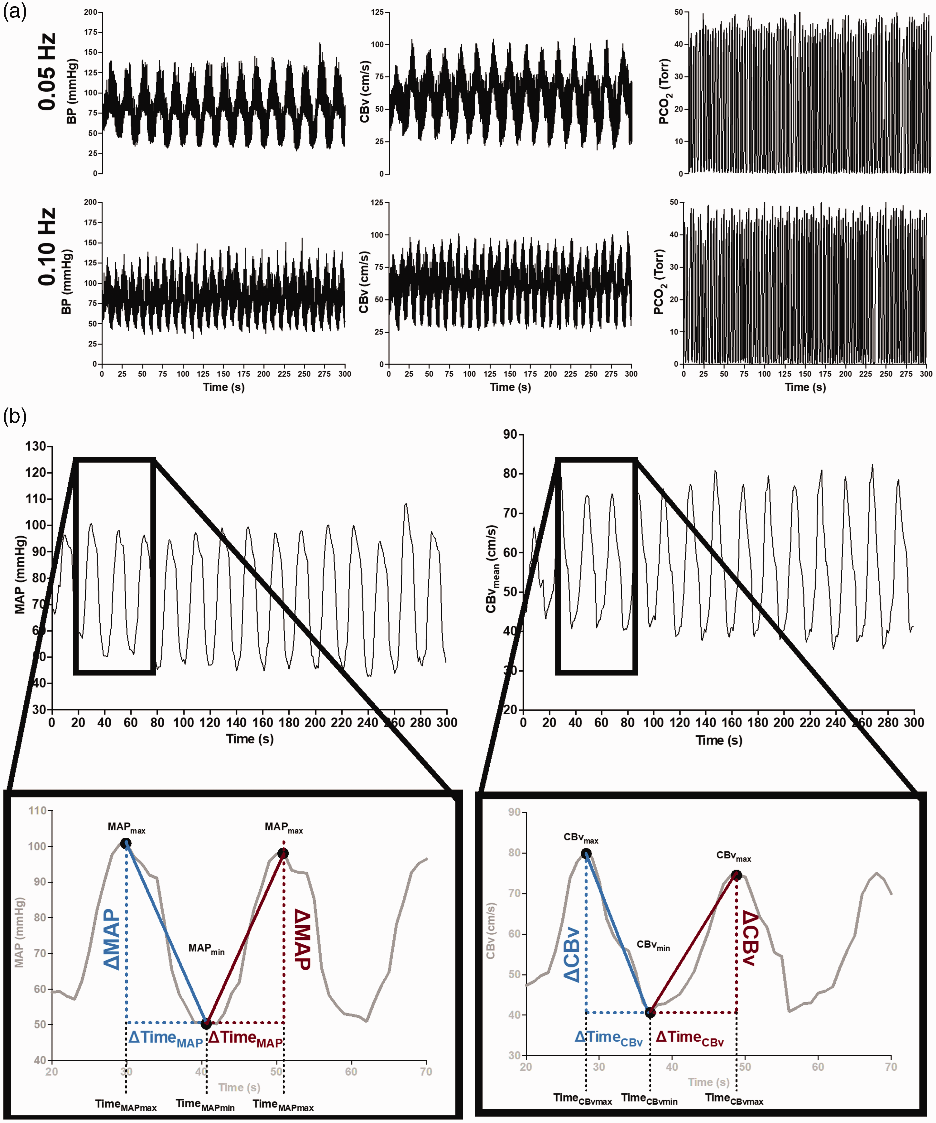
(a) Raw tracings of BP, cerebral blood velocity (CBv) (monitored in the middle cerebral artery), and PCO₂ at 0.05-Hz and 0.10-Hz repeated squat-stands. (b) schematic tracings of MAP and CBv during a repeated squat-stand performed at 0.05 Hz. Enlarged regions depict how the variables were used to calculate ΔCBv_T/ΔMAP_T. Blue color indicates variables used to calculate ΔCBv_T/ΔMAP_T during acute decreases in MAP. Red color indicates variables used to calculate ΔCBv_T/ΔMAP_T during acute increases in MAP. ΔMAP_T, absolute change in MAP; ΔCBv_T, absolute change in CBv; MAP_max, maximum MAP; MAP_min, minimum MAP; CBv_max, maximum CBv; CBv_min, minimum CBv; Time_MAPmax, time at maximum MAP; Time_MAPmin, time at minimum MAP; Time_CBvmax, time at maximum CBv; Time_CBvmin, time at minimum CBv; ΔMAP, absolute change in MAP from minimum to maximum or from maximum to minimum; ΔCBv, absolute change in CBv from minimum to maximum or from maximum to minimum; ΔTime_MAP , time interval between minimum to maximum or between maximum to minimum MAP; ΔTime_CBv, time interval between minimum to maximum or between maximum to minimum CBv. Modified with permission of P. Brassard from. ⁸⁷

Finally, the time-adjusted ratio 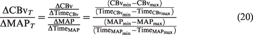$\frac{\Delta \mathrm{CB}{\mathrm{v}}_{\mathrm{T}}}{\Delta \mathrm{MA}{\mathrm{P}}_{\mathrm{T}}}$ during decreases in MAP can be calculated as follows:

$$\frac{{\Delta \mathrm{CBv}}_T}{{\Delta \mathrm{MAP}}_T}=\frac{\frac{\Delta \mathrm{CBv}}{{\Delta \mathrm{Time}}_{\mathrm{CBv}}}}{\frac{\Delta \mathrm{MAP}}{{\Delta \mathrm{Time}}_{\mathrm{MAP}}}}=\frac{\frac{({\mathrm{CBv}}_{\min }-{\mathrm{CBv}}_{\max })}{{(\mathrm{Time}}_{{\mathrm{CBv}}_{\min }}-{\mathrm{Time}}_{{\mathrm{CBv}}_{\max }})}}{\frac{({\mathrm{MAP}}_{\min }-{\mathrm{MAP}}_{\max })}{({\mathrm{Time}}_{\mathrm{MA}{\mathrm{P}}_{\min }}-{\mathrm{Time}}_{{\mathrm{MAP}}_{\max }})}}$$

(20)

During MAP increases, the same quantity can be calculated as:

$$\frac{{\Delta \mathrm{CBv}}_T}{{\Delta \mathrm{MAP}}_T}=\frac{\frac{\Delta \mathrm{CBv}}{{\Delta \mathrm{Time}}_{\mathit{CBv}}}}{\frac{\Delta \mathrm{MAP}}{{\Delta \mathrm{Time}}_{\mathit{MAP}}}}=\frac{\frac{({\mathrm{CBv}}_{\max }-{\mathrm{CBv}}_{\min })}{{(\mathrm{Time}}_{{\mathrm{CBv}}_{\max }}-{\mathrm{Time}}_{{\mathrm{CBv}}_{\min }})}}{\frac{({\mathrm{MAP}}_{\max }-{\mathrm{MAP}}_{\min })}{({\mathrm{Time}}_{{\mathrm{MAP}}_{\max }}-{\mathrm{Time}}_{{\mathrm{MAP}}_{\min }})}}$$

(21)

Of note, values obtained from equations (20) and (21) can be converted to percent changes as described in. ⁸⁴

In addition to reporting directional sensitivity in the middle cerebral artery flow territory,^84,87,88 and the posterior cerebral artery flow territory ⁸⁴ using this metric, the hysteresis-like pattern has been shown to be highly reproducible within the same day. ⁸⁴ It has been associated with a frequency-dependent nature (i.e., present during 0.10 Hz, but not during 0.05 Hz repeated squat-stands), as well as aerobic fitness levels, based on experimental data from healthy participants, young sedentary and endurance-trained volunteers.^84,87,88,90 However, the absence of such a phenomenon has been reported in young individuals habitually trained in resistance exercise. ⁸⁸ Panerai et al. ⁸⁶ have also reported a better autoregulatory response, using the ARI, during transient MAP increases (i.e., during the squatting phase) with the repeated squat-stand model performed only at 0.05 Hz.

Of note, one previous study reported the absence of directional sensitivity in the cerebral pressure-flow relationship. ¹⁵⁸ These authors utilized repeated thigh-cuffs inflations and deflations to produce transient changes in MAP. ¹⁵⁸ While thigh-cuff deflations have been employed in several studies, it has been shown this technique yields variable results and poor reproducibility for dCA metrics, even when assessments are completed just a few minutes apart. ¹⁵⁹ Overall, whether one of the main (or partial) reasons for the occurrence of directional sensitivity of the pressure-flow relationship is the specific approach to induce MAP changes remains to be clarified. However, recent findings ¹⁶⁰ suggest that 5 minutes of lower body negative pressure oscillating between 0 and −83 Torr, using the same calculation methods previously described,^{57,84,87,88,90}can detect directional sensitivity in the cerebral pressure-flow relationship at 0.10 Hz, but not at 0.05 Hz.

Recently, a new approach for identification of directional sensitivity of the dynamic CA response was proposed ⁹¹ using a multivariate ARX approach, which separates the MAP signal into two components, one containing only the beat-to-beat positive derivative information and the other the corresponding time-series of the negative derivative. The main advantage of this approach is that it is fairly general, and that it can be applied to spontaneous fluctuations of MAP at rest, as well as to changes in MAP induced by the squat-stand or other maneuvers. This study demonstrated the presence of directional sensitivity at rest, of similar magnitude as that observed during squat-stand maneuvers at 0.05 Hz. This new method requires further validation, in comparison with other indices proposed for quantification of directional sensitivity, as well as its potential to describe the behaviour of directional sensitivity in different physiological and pathological conditions.

Recommendations:

Considering the relatively limited research related to the directional sensitivity of the cerebral pressure-flow relationship and the diverse modelling approaches used by different investigators, we are unable to comment on a gold-standard approach at the current time but are able to provide the following general recommendations for future research:

Directional sensitivity should be considered in the design and interpretation studies of dCA.

Spontaneous, or forced MAP oscillations using repeated squat-stands or oscillatory lower body negative pressure, are suitable experimental protocols to assess directional sensitivity of the cerebral pressure-flow relationship.

Directional sensitivity can be identified by different analytical methods, such as the ΔCBv_T/ΔMAP_T ratio, ARMA/ARX models and the autoregulatory gain between CBv and MAP by considering MAP increases and decreases separately.

Directional sensitivity should be investigated as a potential significant contributor to the considerable variability in dCA measures over time and between individuals.

Further work is needed to better understand the clinical significance of directional sensitivity metrics for dCA quantification and whether these metrics may improve our ability to predict clinical outcomes.

Recommendations for further research also includes examination of whether the hysteresis-like pattern:

•  ○ is model-dependent (i.e., only present using repeated squat-stand maneuvers).

•  ○ is reproducible between days.

•  ○ remains present in physiological (e.g., hyperthermia, hypoxia) and pathological states (e.g., mild traumatic brain injury, stroke, heart failure) and whether it is influenced by biological sex, aging, blood gases, body position, etc.

Multiple-input models

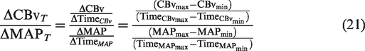
One intrinsic problem with the one-input models previously described is the assumption that CBv is modulated solely by MAP. It is well established, though, that arterial CO₂ (and to a lesser extent arterial O₂) tension can produce significant effects on CBv^{147,161 –164} by exerting changes on the cerebral vasculature. Therefore, several studies have considered multiple-input models, whereby breath-to-breath PETCO₂ and/or end-tidal oxygen tension (PETO₂) are included as indirect measures of arterial CO₂ and O₂ tension to assess their impact on CBv regulation.^{41,42,44,45,47,50 –55,67,68,92 –94,104 –106,149,165} Apart from PETCO₂ and PETO₂, other factors such as body posture,^166,167 heart rate,^54,166 respiration, endocrine and metabolic effects^149,168 have also been shown to affect dCA.

Here, we describe extensions of the single-input (MAP), single-output (CBv) LTI models to two-input, single-output models, whereby both MAP and breath-to-breath PETCO₂ variations are considered as inputs. These models can easily be adjusted to more than two inputs.

Two-input, single-output, linear time invariant systems

A two-input, single-output LTI system can be expressed as,

$$y\left(n\right)=\sum _m^{\mathrm{\infty }}{h}_x\left(m\right)x(n-m)+\sum _m^{\mathrm{\infty }}{h}_z\left(m\right)z(n-m)+\epsilon \left(n\right)$$

(22)

where $x\left(n\right),\mathrm{ }z\left(n\right)$ are the two inputs, and $y\left(n\right)$ is the observed output. In dCA, the variables $x\left(n\right),\mathrm{ }z\left(n\right)$ typically represent MAP and PETCO₂ signals and $y\left(n\right)$ represents CBv. $h_x\left(m\right)$ , $h_z\left(m\right)$ are the system impulse responses that describe the dynamic MAP-CBv and PETCO₂-CBv relationship respectively (Figure 5), whereby the latter is typically referred as cerebrovascular reactivity in the literature, and $\epsilon \left(n\right)$ reflects the effects of measurement noise and unobservable factors. dCA can be assessed based on the estimated MAP-CBv relationship (i.e., $h_x\left(m\right)$ ), as in the single-input case. However, the inclusion of PETCO₂ time-series data $z\left(n\right)$ as a second input accounts for the CO₂ effects upon the dynamic relation between MAP and CBv, since CO₂ is a known potent vasodilator. If the dynamic effects of CO₂ variations upon CBv variations are not considered, the “apparent” estimated model of the MAP-to-CBv relation may be distorted by the effects of CO₂, particularly in the lower frequency range. ⁵³ Therefore, by modelling and removing CO₂ reactivity from the system (through $h_z\left(m\right)$ ), a less biased estimate of the impulse response $h_x\left(m\right)$ and thus more accurate dCA indices are expected.

Figure 5.

Two-input, single-output system. $h_x\left(m\right)$ is the impulse response that describes dCA as the dynamic relationship between MAP and CBv, whereas $h_z\left(m\right)$ describes the dynamic relationship between PETCO₂ and CBv. dCA can be assessed based on the characteristics of $h_x\left(m\right)$ . The inclusion of PETCO₂ as a second input provides a less biased estimate of $h_x\left(m\right)$ , since the effects of PETCO₂ on CBv are accounted for by $h_z\left(m\right)$ .

In the following sections we extend the single-input models described in section Linear Time Invariant systems, to two-input models. The recommendations are the same in both cases, however we provide at the end of this section some general practical guidelines related to the inclusion of the PETCO₂ signal as a second input.

Finite impulse response (FIR) models

As in the single-input case, equation (22) can be implemented as a FIR model, assuming that the impulse responses of the system have a finite duration.^47,92 Therefore, the CBv signal can be expressed as,

$$y\left(n\right)=\sum _{m=0}^{M_x}{h}_x\left(m\right)x(n-m)+\sum _{m=0}^{M_z}{h}_z\left(m\right)z(n-m)+\epsilon \left(n\right)$$

(23)

where $M_x, M_z$ (the filter orders) are the length of the impulse responses $h_x\left(m\right)$ (describing the MAP-CBv relationship) and $h_z\left(m\right)$ (describing the PETCO₂-CBv relationship), respectively.

Direct estimation of impulse responses

An optimal estimate of $h_x\left(m\right)$ and $h_z\left(m\right)$ in equation (23) can be obtained using the mean-square error estimator:

$$\widehat{\mathit{h}}=\left[{\widehat{\mathit{h}}}_{\mathit{x}} {\widehat{\mathit{h}}}_{\mathit{z}}\right]={\left[\begin{array}{cc}{\mathit{R}}_{xx}& {\mathit{r}}_{zx}\\ {\mathit{r}}_{xz}& {\mathit{R}}_{zz}\end{array}\right]}^{-1}\left[\begin{array}{c}{\mathit{r}}_{xy}\\ {\mathit{r}}_{zy}\end{array}\right]$$

(24)

where $\left[\begin{array}{cc}{\mathit{R}}_{xx}& {\mathit{r}}_{zx}\\ {\mathit{r}}_{xz}& {\mathit{R}}_{zz}\end{array}\right]$ is the input correlation matrix composed of the auto- (i.e., ${\mathit{R}}_{xx},{\mathit{R}}_{zz}$ ) and cross-correlation matrices (i.e., ${\mathit{r}}_{xz}$ , ${\mathit{r}}_{zx}$ ) of $\mathit{x}$ and $\mathit{z}$ . ${\mathit{r}}_{xy}$ and ${\mathit{r}}_{zy}$ , are the cross-correlation matrices between $\mathit{x}$ and $\mathit{y}$ and $\mathit{z}$ and $\mathit{y}$ , respectively. The least squares solution using the Moore-Penrose pseudoinverse can also be applied here (see Supplementary Material, Eq. (S3)). Once $\widehat{\mathit{h}}$ has been estimated, dCA is quantified based on ${\widehat{\mathit{h}}}_{\mathit{x}}$ (as in the single-input case).^47,92 By using two-input FIR models, Panerai et al. ⁴⁷ observed a strong effect of PETCO₂ on CBv during free-breathing conditions. However, the MAP-CBv relationship was not found to be affected significantly by the inclusion of PETCO₂. This was explained by the fact that spontaneous PETCO₂ fluctuations may not exert significant influences on dCA, with PETCO₂ fluctuations found predominantly at very low frequencies. However, later studies reported less variable dCA estimates especially in the very low frequency range (below 0.07 Hz), where the PETCO₂-CBv relationship was also found to be nonlinear and time-varying.^53,104

Estimation of impulse response functions through Laguerre expansions

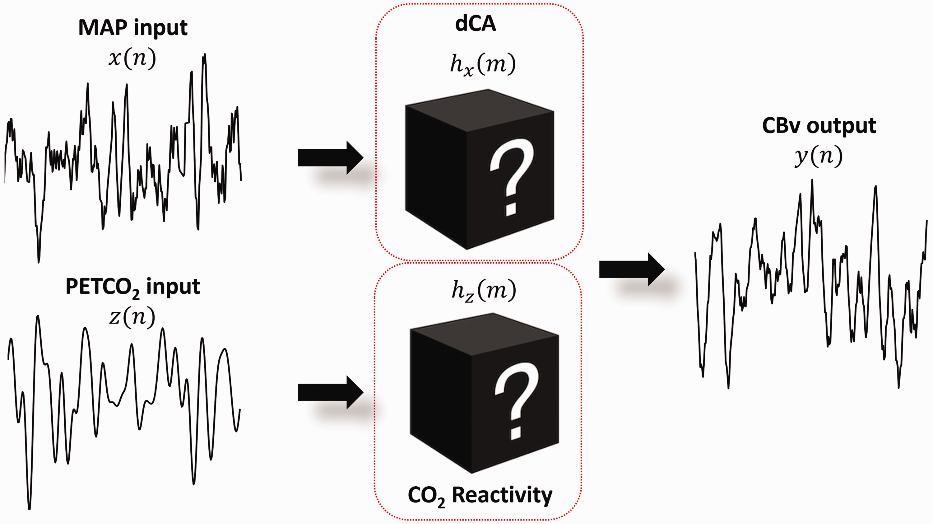
The LET approach was presented earlier as a robust method for estimation of the impulse response function of a LTI system with a single input.^39,40 The LET can also be applied to the estimation of nonlinear time-invariant and multi-input models. In the context of LTI modeling of dCA, breath-to-breath variations of PETCO₂ can be added as a second input. Thus, the output CBv signal $y\left(n\right)$ is expressed as the sum of two convolutional terms involving the two input signals, MAP and PETCO₂, denoted by $x\left(n\right)$ and $z\left(n\right)$ , respectively, with the corresponding impulse responses $h_x\left(m\right)$ and $h_z\left(m\right)$ as in equation (23).

To estimate the kernels $h_x\left(m\right)$ and $h_z\left(m\right)$ in equation (23) using input-output data, we expand them on two bases of DLFs, $\left\{b_j^x\right\}$ and $\left\{b_j^z\right\}$ respectively, with distinct Laguerre parameters “alpha” (determined from the data), as:

$$h_x\left(m\right)=\sum _j{c}_j^x{b}_j^x\left(m\right),\mathrm{ }{h}_z\left(m\right)=\sum _j{c}_j^z{b}_j^z\left(m\right)$$

(25)

where $\left\{c_j^x\right\}$ and $\left\{c_j^z\right\}$ denote the Laguerre expansion coefficients of the two impulse responses to be estimated from the data via linear (least-squares) regression. The number of required DLFs for each kernel expansion and the respective parameters alpha are determined through a search procedure that minimizes the BIC criterion (see Supplementary Material, section II. 2.2). The LET, shown in equation (25), transforms the model of equation (23) into equation (26), where the time-series $\left\{v_j^x\right(n\left)\right\}$ and $\left\{v_j^z\right(n\left)\right\}$ are convolutions of each input with the respective Laguerre basis functions (see Supplementary Material, section II. 2.2):

$$y\left(n\right)=\sum _j{c_j^{x}v}_j^x\left(n\right)+\sum _j{c_j^{z}v}_j^z\left(n\right)+\epsilon \left(n\right)$$

(26)

Equation (26) depends on the unknown Laguerre expansion coefficients linearly; hence these coefficients can be estimated via linear regression. This two-input modeling approach has found successful application in several studies of dCA to date.^{41,42,50,53 –55,68,93}

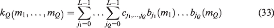
As an illustrative example, we show in Figure 6 the average impulse response estimates and their standard deviation bounds for MAP (Figure 6(a)) and PETCO₂ (Figure 6(b)), obtained via the LET from 5-min time-series measurements of 20 healthy elderly adults (10 female & 10 male, 60–75 years old, without cardiovascular disease, diabetes, arterial hypertension or cognitive impairment), using 4 DLFs for each kernel. ⁵⁵ The relatively tight SD bounds, for relatively short data-records (5 min) of highly noisy data, corroborate the efficacy of the LET estimation method.

Figure 6.

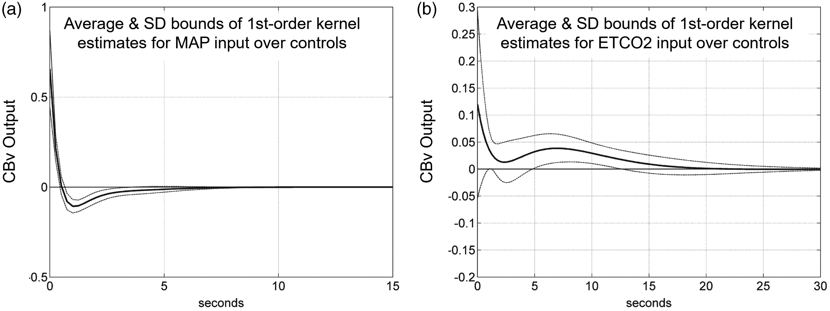
Average estimated impulse response function between (a) MAP (input) and CBv (output) and (b) PETCO₂ (input) and CBv (output) obtained via the LET for a group of healthy elderly adults. Modified with permission from ⁵⁵ under the Creative Commons CC-BY license.

Infinite impulse response (IIR) models

A two-input ARX structure of order ( $n_a$ , $n_b,n_d$ ) is defined as,

$$y\left(n\right)=\sum _{m=1}^{n_a}{a}_{m}y(n-m)+\sum _{m=0}^{n_b}{\beta }_{m}x(n-m)+\sum _{m=0}^{n_d}{d}_{m}z(n-m)+\epsilon \left(n\right)$$

(27)

where the output $y\left(n\right)$ is CBv, the exogenous (X) inputs $x\left(n\right)$ and $z\left(n\right)$ are assumed to be the MAP and PETCO₂ signals, and the autoregressive (AR) counterpart $y(n-m)$ refers to the CBv history. As in the FIR case, the ARX coefficients { $a_m$ }, { ${\beta }_m$ } and { $c_m$ } can be estimated using the least squares technique. Kostoglou et al. ⁶⁷ used time-invariant three-input ARX models to capture dCA characteristics in young athletes following concussion. The three inputs were MAP, PETCO₂ and visual stimulation during visual/mental tasks.

In a similar manner, the two-input ARMAX ( $n_a$ , $n_b,n_d,n_c$ ) model can be expressed as,

$$y\left(n\right)=\sum _{m=1}^{n_a}{a}_{m}y(n-m)+\sum _{m=0}^{n_b}{\beta }_{m}x(n-m)+\sum _{m=0}^{n_d}{d}_{m}z(n-m)+\sum _{m=1}^{n_c}{c}_m\epsilon (n-m)+\epsilon \left(n\right)$$

(28)

The OE approach can also be extended to a two-input model as follows,

$$\xi \left(n\right)=\sum _{m=1}^{n_a}{a}_m\xi (n-m)+\sum _{m=0}^{n_b}{b}_{m}x(n-m)+\sum _{m=0}^{n_c}{c}_{m}z(n-m)$$

(29)

$$y\left(n\right)=\xi \left(n\right)+\epsilon \left(n\right)$$

(30)

where $\xi \left(n\right)$ is an auxiliary signal, $y\left(n\right)$ is the observed CBv output and $x\left(n\right)$ and $z\left(n\right)$ are the MAP and PETCO₂ inputs, respectively. $\epsilon \left(n\right)$ is assumed to be additive measurement noise.

To our knowledge, two-input ARMAX and OE models have not been applied for dCA analysis. Nonetheless, it would be of interest in the future to compare the analysis results with these types of approaches, as these model types are theoretically more suitable for handling non-white residuals.

Pure time delays

CBv exhibits a pure-time delay in its response to PETCO₂ changes,^{47,162,165,169} due to measurement (e.g., length of capnography tube used to measure the concentration of expiration CO₂) and physiological delays. In Figure 7(a), we illustrate the time-varying cross-correlation coefficient $$ between PETCO₂ and CBv computed using 160 s sliding windows from 40 min of resting data. ¹⁰⁹ Maximum values occur at negative lags and in the range of [−3 −15] s, indicating that CBv responses are delayed in comparison to PETCO₂. This can be taken into account by shifting the time-series accordingly or adding a constant pure-time delay factor $d$ to the PETCO₂ component of equation (23),

$$y\left(n\right)=\sum _m^{\mathrm{\infty }}{h}_x\left(m\right)x(n-m)+\sum _m^{\mathrm{\infty }}{h}_z\left(m\right)z(n-m-d)+\epsilon \left(n\right)$$

(31)

Figure 7.

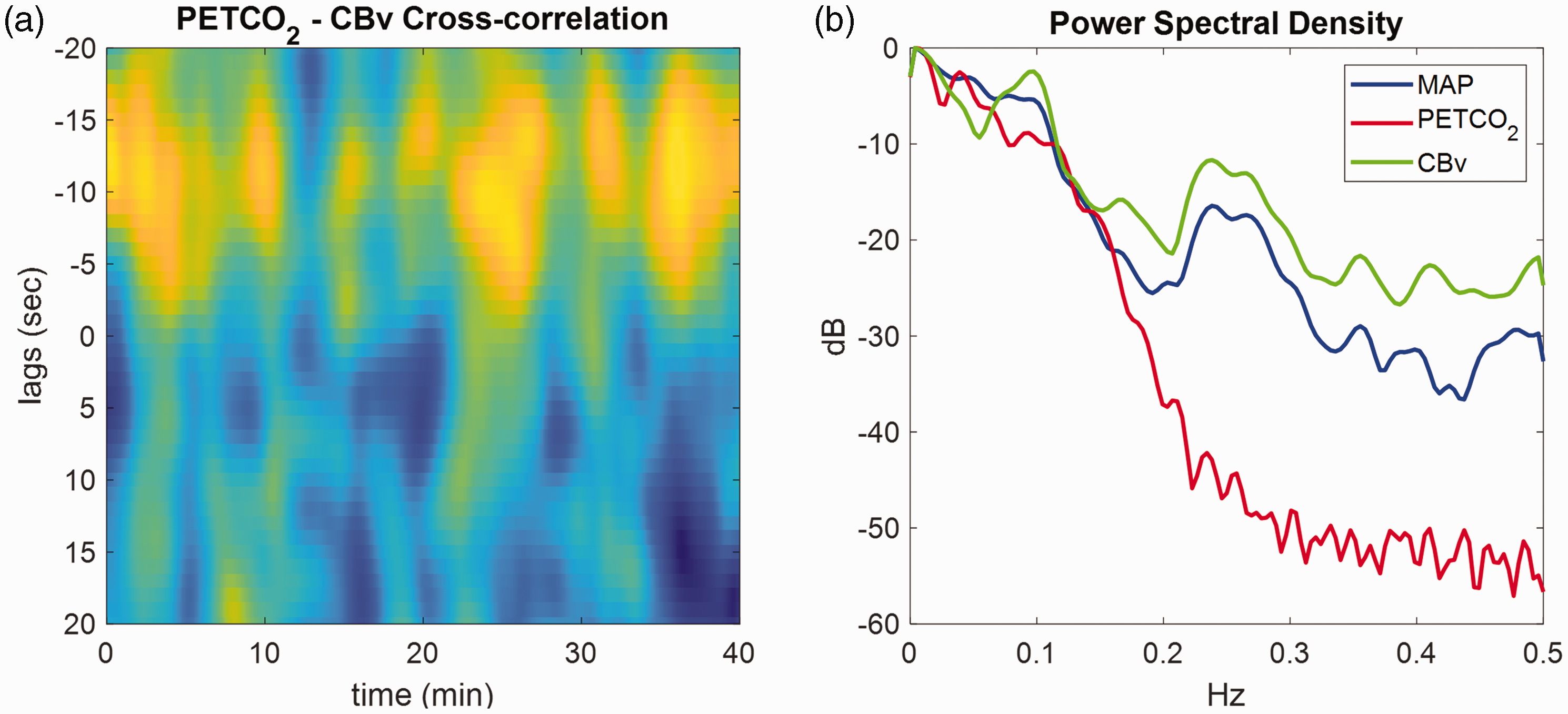
(a) Time-varying cross-correlation coefficient between PETCO₂ (breath-to-breath data) and CBv (both sampled at 1 Hz) obtained during 40 min of spontaneous fluctuations, estimated using overlapping sliding windows of 160s. The x-axis represents time in seconds and the y-axis the lags of the cross-correlation function. Peaks (yellow) at negative lags indicate delayed CBv response compared to the PETCO₂ signal. The pure time delay corresponding to the effects of PETCO₂ on CBv range between 3 to 15s and (b) Power spectral density (in dB) of the corresponding MAP (blue), PETCO₂ (red) and CBv (green) signals.

Usually, $d$ is set to a fixed value of 3–6 s^{47,53,162,169,170} based on the length of the capnography tube. However, it can be optimized along with the model structure using cross-validation or model order selection criteria. Note that $d$ does not affect the total number of free parameters; however, its selected value may affect the final model fit and influence model order selection. Therefore, for a fixed model structure, the optimal delay is the value that corresponds to the minimum MSE between actual and predicted CBv output. It is important to note, however, that this approach may not work effectively if the measurement noise has a colored structure. In other words, if the measurement noise has a specific pattern or correlation, it can interfere with the accuracy of the predicted CBv output, and the optimal delay may not be achieved. Although the delay is usually assumed to be constant, variations are also evident in Figure 7(a). These could be due to physiological factors or poor SNR ratio between PETCO2 and CBv within some windows.

Recommendations:

To improve model fitting in the case of two-input models with PETCO₂ as the second input, the use of a pure time delay in the CO₂ model component is recommended. Estimation of pure time delays for PETCO₂ should be performed using experimental data segments with a sufficient PETCO₂-to-CBv SNR. If such data are not available, using a delay between 3–6 s is reasonable.

Since PETCO₂ power is concentrated in frequencies below 0.15 Hz (Figure 7(b)) (and in most cases below 0.1 Hz), we recommend downsampling all signals to 1 Hz to include both cardiac and respiratory cycles without introducing increased PETCO₂ signal collinearities due to oversampling. If the model of analysis allows for multiple sampling frequencies (e.g., FIR models), different sampling rates may be used for each input. For example,^47,92 employed a multi-rate FIR approach, whereby MAP was downsampled to 1 Hz and PETCO₂ to 0.2 Hz.

Extensions

Nonlinear models

Nonlinearities are common in many physiological systems. In dCA, nonlinearities arise mainly due to changes in cerebrovascular resistance, but also due to the influence of various metabolic, neurogenic and myogenic mechanisms.^149,168 Some TFA studies have reported low coherence values between MAP and CBv in the very low frequency range (<0.07 Hz).^18,25 This has been attributed to intrinsic nonlinearities, though their effects likely overlap with the main effects of PETCO₂ on CBv in the frequency domain.^{42,50,53 –56,93,95,98 –101} Nonlinear models yield improved CBv prediction accuracy performance; however, this comes at the cost of increased complexity. The increased number of model parameters necessitates also longer data recordings to ensure robust estimation and reduce the risk of overfitting. Furthermore, the lack of a consensus regarding optimal nonlinear indices of dCA effectiveness has rendered the use of nonlinear models more limited. In the following sections, we provide an overview of the most commonly used nonlinear time-domain models in an effort to elucidate their main technical aspects.

Volterra-type models

The input-output relationship of a $Q$ -th order, nonlinear, single-output system can be expressed by the following Volterra model in discrete time: ⁴⁰

$$y\left(n\right)=k_0+\sum _m{k}_1\left(m\right)x\left(n-m\right)\sum _{m_1,m_2}{k}_2\left(m_1,m_2\right)x\left(n-m_1\right)x\left(n-m_2\right)+\dots +\sum _{m_1.m_Q}{k}_Q\left(m_1,\dots ,m_Q\right)x\left(n-m_1\right)\dots x\left(n-m_Q\right)$$

(32)

where $x\left(n\right)$ is the MAP input and $y\left(n\right)$ is the CBv output, and $k_Q\left(m_1,\dots ,m_Q\right)$ are the $Q$ -th order Volterra kernels of the system. Volterra kernels are weighting functions that describe the effect of past input values (linear kernel), as well as the effect of the $Q$ -th order products between past input values to generate the output signal. The zeroth-order Volterra kernel ( $Q$  = 0) is the output of the system when all inputs are absent. The first-order ( $Q$  = 1) and higher order kernels ( $Q$  > 1) capture the linear and nonlinear dynamics of the system, respectively. As in the single- and multiple- input linear case, these kernels can be efficiently estimated using LET. ³⁹ Specifically, the discretized Volterra kernels of the system can be expanded in terms of the orthonormal basis of DLFs as follows:

$$k_Q\left(m_1,\dots ,m_Q\right)=\sum _{j_1=0}^{L-1}\dots \sum _{j_Q=0}^{L-1}{c}_{j_1,\dots ,j_Q}{b}_{j_1}\left(m_1\right)\dots b_{j_Q}\left(m_Q\right)$$

(33)

A more compact and interpretable representation of the Laguerre-Volterra model is the Principal Dynamic Modes (PDM) model.^40,171 The PDM model hypothesizes that the underlying dynamics can be adequately captured by a minimum number of filters (i.e., PDMs) followed by a static nonlinearity. The PDMs are obtained by applying singular value decomposition on the estimated Volterra kernels of the system (equation (33)). The PDM model is an interpretable structure that can provide valuable physiological insights.^42,54,55,93 Marmarelis et al. ⁴² employed the PDM approach to describe nonlinear dCA dynamics in a cohort of 12 healthy subjects. The extracted ‘global’ PDMs (i.e., PDMs estimated using data from all participants) were found to be relatively robust to inter-subject variability.

In,^50,172,173 Mitsis et al. proposed the Laguerre Volterra Network, which combines the LET approach with feedforward artificial neural networks (ANN). It consists of three layers: the input layer, the hidden layer, and the output layer. In the input layer, the input is processed by a Laguerre filter-bank. The output of the filter-bank is then fed into the hidden layer through weighted connections. The hidden layer consists of hidden units characterized by polynomial activation functions. The final output, in the output layer, is computed as the non-weighted sum of the hidden unit responses. The weights of the network can be trained using iterative approaches such as back-propagation. The resulting model is computationally more efficient, providing a more parsimonious description of the underlying dynamics compared to the standard Laguerre Volterra model of equation (32).

Recommendations:

Model order/structure determination is particularly important in the case of nonlinear models. In the case of Laguerre-Volterra models, apart from the number of DLFs and the Laguerre parameters ‘alpha’, the order of nonlinearity $Q$ significantly affects the results. According to previous results, it seems that using $Q=2$ is sufficient in the case of dCA. In the case of Laguerre Volterra Networks, the number of hidden units should also be defined. Similar recommendations to linear models apply here. Cross-validation or model order selection criteria can be used to optimally select these hyperparameters. Please refer to the Supplementary Material (section II. 2.2) for more details.

Artificial neural networks, autoregressive support vector machines and time genetic models

Machine learning is showing rapid progress in a wide range of contexts. ANNs, Support Vector Machines (SVMs) and Time Genetic Models (TGMs) are applications relying on supervised learning. A simple example of supervised learning was reported by Panerai et al. for the automatic classification of dCA responses in premature neonates. ¹⁷⁴ One of the advantages of these structures is the possibility to model dCA as either a linear or a non-linear process.^{99 –103,167} All three types of models allow multiple variables as inputs but are restricted to a single output. The non-linear capabilities of these models also allow spontaneous MAP variations to be used for learning other behaviours such as sit-to-stand,^175,176 squat-stand, or Valsalva maneuvres. However, it is important to note that these maneuvres typically last around 1 minute while spontaneous variations are recorded over longer time windows. ¹⁸

In their original formulation, and common applications to other fields, ANNs and SVMs were used to model static phenomena. However, it has been shown that by extending their structures to allow dynamic behaviour, they can successfully model dCA.^{98 –100} As for TGM, it has been shown that it can be an efficient approach to identifying parameters in linear and non-linear biophysical models.^102,103

In general, for all three methods, parameter search is realised by means of a grid covering the entire search space, for each subject. Using an ad-hoc grid interval for each case, the model is inspected, in each of the two folds of the balanced cross-validation, ¹³³ to select the best evaluated model in the test set. The parameters to be selected for ANNs and SVMs can be separated into two types: internal parameters (also called hyperparameters) and external delays corresponding to the order of previous time lags of the different modelled signals, as in the case of CBv, where these correspond to the order of the model.

Hyperparameters – ANNs: Here only two internal parameters (or hyperparameters) need to be set: the size of the hidden layer and the activation functions of the neurons in this layer (the same function is used for all neurons). The hidden layer is the layer between the input and the output of the network and its primarily purpose is to nonlinearly transform the input data based on a predefined activation function. The size of the hidden layer is determined by the number of neurons in this layer, which in turn affects the complexity of the network.

Hyperparameters – SVMs: For a static regression SVM, the hyperparameters are the support vector penalties termed C costs, the nonlinear kernel function and the size of the support vector zone. The C cost is a regularization parameter that balances the trade-off between maximizing the margins between the support vectors and minimizing the prediction error. The size of the support vector zone is indirectly controlled by the C cost. A larger value of C leads to a smaller margin and thus a smaller support vector zone. The kernel function defines the type of nonlinearity. Commonly used kernel functions include linear, polynomial and radial basis functions. These hyper-parameters are selected using a grid of values in powers of two as proposed in. ¹⁷⁷

In addition to these internal parameters, the time delays for each signal are required. A non-linear temporal model, where the dependent variable is CBv (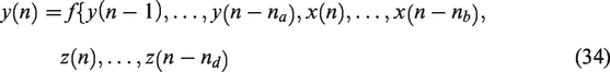 $y\left(n\right)$ ) and the two inputs are MAP ( $x\left(n\right)$ ) and PETCO₂ ( $z\left(n\right)$ ), can be written as:

$$y\left(n\right)=f\{y\left(n-1\right),\dots ,y\left(n-n_a\right),x\left(n\right),\dots ,x\left(n-n_b\right),z\left(n\right),\dots ,z\left(n-n_d\right)$$

(34)

where $f$ is the nonlinear function described by the ANN or SVM. In this model, $n_a,n_b$ and $n_d$ are required to be set. Values are searched using a cross-validation strategy following the recommendations provided in section Infinite Impulse Response (IIR) models for all parameter combinations.

Hyperparameters – TGMs: The ARX structure is based on a high pass filter using resistive (R_i) and capacitive elements (C_i) and the hydraulic-electric analogy^102,103 in which the ABP corresponds to the voltage source and CBv to the total current (Supplementary Material, section IV, Fig. S3 top panel).

The TGM approach, considers physiological constraints for cerebrovascular resistive (R_i) and compliance (C_i) values within the model, which are presented as chromosomes within the TGM population (Supplementary Material, section IV, Fig. S3 bottom panel). These chromosomes are then optimized using genetic algorithms. Genetic algorithms require tuning of several hyperparameters including the population creation function, the population number, the generations, as well as the crossover/mutation operators to achieve optimal performance. To find the best configuration a grid search can be used and an optimisation criterion for fitting the models can be defined (e.g., mean square error between measured and estimated CBv). Finally, each method has its own regularisation approach for building the models.

Recommendations:

For the three methods described above, the signals should be pre-processed in the same way as indicated in recommendations #1–#7 of ²⁶ (i.e., CBv, MAP and PETCO₂ signal lengths of 5 min and sampling rates ≥5 Hz).

For ANN and SVM, the signals should be normalised within the range [0–1]. In the case of TGM, the signals should be demeaned.

It is recommended to use balanced cross-validation ¹³³ for training or two fold cross-validation as explained in section Infinite Impulse Response (IIR) models (see also Supplementary Material, section II. 1.1).

Model order selection can be performed using two criteria:

•  ○ Pearson's correlation coefficient and the MSE between measured and estimated CBv should be calculated to assess model accuracy. ¹⁴²

•  ○ The model-predicted CBv response to a normalised MAP step as input. A model should be considered as valid if this response is physiologically plausible. This can be done according to the recommendations given in. ¹⁴² The general criteria for rejecting CBv responses are: “(a) negative initial value, (b) monotonically rising, (c) slow or delayed initial rise, (d) oscillatory with growing amplitude and (e) large negative final value in comparison with the initial peak”^73,142

•  ○ The final selected model is the one that achieves the highest accuracy while fulfilling the physiological criteria outlined above.

Time-varying models

The techniques described in the previous sections rely on the assumption that the MAP & CBv relationship remains constant over time, which may not be the case. If this relationship changes over time, a time invariant model will capture its average behavior within the observed period. ¹⁰⁴ However, previous studies have suggested that dCA exhibits time-varying characteristics,^{19,46,49,53,61,66,104 –111,113 –115,117,170,178 –180} though it is still unclear whether this behavior mainly reflects inherent systemic time-varying behavior or the effect of unobservable factors. Temporal dCA variability has been mainly attributed to external physiological mechanisms (e.g., autonomic nervous system activity or body temperature), unobservable factors (e.g., PETCO₂ effects not taken into account) and variations in the experimental conditions (e.g., free-breathing conditions followed by sustained euoxic hypercapnia or repeated maneuvers/changes in posture). Interestingly, in Marmarelis et al., ¹⁰⁴ the authors observed cyclical CA variations within 6 minutes of resting state recordings, especially in the very low frequencies (below 0.01 Hz). Their main hypothesis was that these variations suggest the potential presence of periodic alterations in the neuroendocrine mechanisms that regulate perivascular smooth muscle tone. Therefore, dCA time-varying behavior could explain the lack of reproducibility in studies where repeated measurements were performed days and weeks apart.^{50,181 –184} To track time-variations in the characteristics of dCA, the most common approaches are the sliding window technique, recursive methods and multimodal pressure-flow analysis. It is important to note that the terms ‘nonstationary’ or ‘time-varying’ are also used to describe signals for which the statistical properties (mean, variance, autocorrelation function) vary over time, but in the present paper we focus on the time-varying behavior of the underlying system (dCA).

Sliding window method

The sliding window technique involves fitting time invariant models to possibly overlapping sliding windows of MAP and CBv data. The obtained dCA indices (e.g., impulse response function, phase/gain estimates) are then interpolated, providing piece-wise constant trajectories of the dCA system characteristics. Although this is a simple and straightforward approach, the selection of an optimal window length is not trivial. A short window may lead to noisy estimates, whereas a long window may smoothen out abrupt and fast changes, underestimating the magnitude and rate of variations in the data. In dCA, typical window lengths are of the order of 60s with a sliding step of 5s.^61,104 In Mitsis et al., ⁵³ the authors used 6-min windows with a 5-min overlap to track the temporal variability of dCA within 40 min of resting data. All of these studies observed time-variations in autoregulatory function even during resting conditions.

Recommendations:

To reduce the computational load, especially if overlapping sliding windows are used, it is recommended to downsample the data to sampling rates of 1 to 5 Hz.

For FIR/IIR models, the average/median model order obtained from all windows should be used as a universal model order for all windows.

The choice of window length involves a balance between accurate tracking and accurate model estimation. The window should be short enough to be able to capture fast variations, but also long enough to correctly identify the underlying system without under- or over-fitting the data. Therefore, the number of unknown model coefficients should be also taken into account.

Recursive methods

An alternative approach, which is applicable to FIR and IIR models, is the use of recursive techniques that provide continuous estimates of the model coefficients. dCA indices can then be extracted at each time point, thus allowing tracking with higher temporal resolution compared to the sliding window approach.^{105 –108,111,180} Recursive methods include Kalman Filtering (KF) ¹⁸⁵ and the Recursive Least Squares (RLS) technique.^43,186 RLS provides recursive estimates of the model coefficients by minimizing a weighted least squares cost function. The RLS forgetting factor $\lambda$ ( $0<\lambda \le 1$ ) defines the rate of adaptation. Values closer to 1 result in slower adaptation rates and a higher degree of smoothing. Values closer to 0, result in faster adaptation but also higher sensitivity to noise. Therefore, the optimal tuning of $\lambda$ is important. On the other hand, the KF assumes that the model coefficients follow a random walk. The magnitude of the changes is dictated by the covariance matrix of the random walk process and the measurement noise variance. An alternative approach is the use of Korenberg’s method ¹⁸⁷ where the time-varying model coefficients are expressed using an orthogonal expansion that captures their dependence on time (Fourier, Haddamard, Legendre polynomials).

Liu et al. ¹⁰⁶ used RLS to estimate the time-varying coefficients of a FIR dCA model during stepwise changes in PETCO₂. They observed a slow decrease in autoregulatory efficiency during induced hypercapnia and a rapid return to normal levels when shifting back to normocapnia (Figure 8(a)). Similar results were reported in, ¹⁰⁵ whereby time-varying two-input (i.e., MAP and PETCO₂) linear Laguerre-Volterra models were used to capture changes in dCA. The model coefficients were updated using RLS with multiple adaptive forgetting factors to take into account different rates of variations for the two inputs. The authors also observed that the inclusion of PETCO₂ as a second input reduced the nonstationarity of the dCA estimates obtained from single-input models. Aoi et al. ¹¹¹ used an ensemble KF approach to estimate online the coefficients of the model described in ⁸¹ during postural transitions from sitting-to-standing, whereas Kostoglou et al. ¹¹⁰ applied both RLS and KF approaches in combination with linear Laguerre Volterra models to describe dCA in patients suffering from vasovagal syncope during a head-up tilt protocol (Figure 8(b)). Finally, Panerai et al. ¹¹² applied Korenberg’s method ¹⁸⁷ to extract time-varying ARI estimates from young and old healthy subjects with a higher temporal resolution compared to the sliding-window approach.

Figure 8.

(a) The mean PETCO₂, CBv and phase lead (PL) at 1/12 Hz from 11 subjects during an hypercapnic step. In the bottom subplot the solid line shows mean phase lead and the dashed-dotted line is the standard deviation. To track variations, the RLS algorithm was used. During hypercapnia, the phase lead decreases indicating decrease in autoregulatory function. On return to normocapnia, a more rapid change in autoregulation is observed. Used with permission of J. Liu from; ¹⁰⁶ permission conveyed through Copyright Clearance Center, Inc and (b) Time-varying MAP and PETCO₂ first-order kernels from a representative subject suffering from vasovagal syncope during a head-up tilt protocol. The blue dashed vertical lines define the onset of the tilting phase. The red vertical dashed lines denote the time of syncope occurrence, and the green dashed lines denote the time point when MAP reached its minimum value. Used with permission of Elsevier and K. Kostoglou from. ¹¹⁰

Recommendations:

For recursive methods, it is essential to remove spurious, impulse-like artifacts from the data (e.g., through clipping or interpolating) since this could affect the instantaneous model coefficient estimates.

For RLS, typical values for the forgetting factor are between 0.90 and 0.99. However, this depends on the length of the data, magnitude of variations, underlying SNR and model complexity. ¹¹⁰ An optimal value can be obtained by sequentially increasing the forgetting factor and estimating the MSE between predicted and actual CBv output. The forgetting factor that corresponds to the minimum MSE should be selected for further analysis. Kostoglou et al.^105,110 used a mixed-integer aenetic algorithm to optimize both model order and forgetting factor values simultaneously. In another approach, Liu et al. ¹⁰⁶ selected the forgetting factor based on the MSE between the estimated phase lead and the ‘reference’ phase lead obtained from Ursino’s model.

KF hyperparameters can be tuned in a similar manner. In KF, accurate tracking requires tuning of the covariance matrix of the random walk process that describes the time evolution of the model coefficients and the measurement noise variance. Details regarding optimal selection of these values can be found in. ¹¹⁰

Although both RLS and KF produce similar results, in ¹¹⁰ it was shown that KF approaches are more appropriate for complex models with a large number of coefficients (e.g., nonlinear models).

Model order selection is not a straightforward procedure in time-varying systems. Usually, a predefined model structure is required prior to applying RLS or KF. This could be acquired for example based on the sliding window approach (i.e., using sliding windows and extracting the average or median model order obtained from all windows ¹⁰⁸ ) Kostoglou et al.^105,110 used a mixed-integer Genetic Algorithm to select both model order and RLS/KF hyperparameters simultaneously by minimizing the BIC/AIC score in the whole dataset.

Multimodal pressure-flow analysis

Multimodal pressure flow (MMPF) analysis was introduced to evaluate dCA dynamics based on instantaneous phase analysis between ABP and CBv oscillations. ¹⁸⁸ The physiological concept behind MMPF is similar to that of TFA: phase shifts between CBv and ABP (or CPP) oscillations at different frequencies reveal the frequency-dependent behavior of dCA. However, different from the TFA, MMPF was proposed to address the fundamental limitations due to the assumptions of the Fourier transform—the key mathematical tool used in TFA: CBv and ABP (or CPP) consist of oscillatory components that have sinusoidal waveforms with constant amplitude and frequency (assuming stationarity). Though it is recommended that coherence should be examined in the TFA to ensure the assumption of the CBv-ABP linear relationship and the reliability of TFA results, the assumptions of stationary and linear couplings may not be valid in many physiological oscillations. As a time-domain analysis technique, MMPF was designed to extract oscillatory components in CBv and ABP (or CPP) signals that may be possibly non-sinusoidal (requiring an infinite number of sinusoidal functions at a fundamental frequency and its harmonics to describe them) and nonstationary, and to examine the instantaneous phases of each CBv oscillatory component and its corresponding ABP oscillatory component (Supplementary Material, section V, Fig. S4). MMPF can be performed on raw ABP (CPP) and CBv (beat-to-beat arterial waveform) or on MAP and mean CBv. However, all previous studies employing MMPF used raw ABP (CPP) and CBv data.

The MMPF method includes four major steps:

The empirical mode decomposition (EMD) or some of its improved variants (e.g., ensemble empirical mode decomposition: EEMD ¹⁸⁹ ) can be used to decompose each signal (ABP and CBv) into multiple oscillatory components, called intrinsic mode functions (IMFs), each spanning a narrow band of frequencies. EMD is the key for performing MMPF because this nonlinear method allows extraction of possibly nonlinear and nonstationary oscillations in a given signal (Supplementary Material, section V, Fig. S4), achieving better performance than the Fourier transform and the wavelet transform.^188,190

For each oscillatory component or IMF in CBv, its corresponding component in ABP is identified (based on the frequency band of the IMF).

The Hilbert transform is used to obtain instantaneous phases (i.e., the phase at each time point) of each pair of IMFs (CBv IMF and the corresponding ABP IMF) and instantaneous phase shifts. In addition, based on the instantaneous phases of ABP (or CBv), the frequency of each cycle in the ABP IMF and instantaneous frequency for each point can be determined.

For each frequency bin of interest (e.g., low frequency band 0.07–0.2 Hz, or high frequency band: 0.2–0.5 Hz), the mean phase shift is obtained from the CBv-ABP phase shifts for all the frequencies within the bin.

It has been shown that MMPF is able to quantify the CBv-ABP phase shifts reliably from spontaneous ABP and CBv oscillations, and the results during resting conditions are comparable to those obtained from the ABP and CBv signals during the Valsalva maneuver (Figure 9). ¹¹⁷ Using the MMPF derived CBv-ABP phases, previous studies have demonstrated altered dCA, as well as its association to health outcome under pathological conditions including hypertension, stroke, diabetes and brain injury.^{113 –117} It is important to note that the current version of MMFF is still focused on linear CBv-ABP (CPP) couplings, though the extracted oscillatory components of ABP and CBv can be used to assess both linear and nonlinear interactions. Indeed, EMD-based methods have been proposed to detect nonlinear couplings in physiological signals such as phase-amplitude coupling and cross-frequency amplitude-amplitude coupling,^191,192 but these methods have not been applied to the study of the CBv-ABP coupling.

Figure 9.

Screen copy of our MMPF analysis software. The data shown in this plot are from a healthy subject. The top three panels on the left show CBv (left side and right side) and ABP signals, respectively. The colored curves in these panels show the results after removing faster fluctuations from the original signals. The bottom left panel shows the corresponding intrinsic modes for these three signals (red: ABP; blue: CBv on right side; green: CBv on left side). The vertical red dashed box (around 40–50 s) identifies the Valsalva maneuver. The spontaneous oscillations in these signals during resting conditions prior to the Valsalva maneuver can also be visualized. One of these oscillations (around 14–22 s) is identified by two vertical red lines. The result of the ABP–CBv phase shift analysis of this period is plotted in the right panel. A reference line (dotted black line), indicating synchronization between ABP and CBv, is shown in this panel for easy comparison. The result is representative of normal autoregulation where CBv leads ABP (by about 50 degrees in phase). Modified with permission from ¹⁸⁸ under the Creative Commons CC-BY license.

Recommendations:

The optimized algorithm of the EMD published by ¹⁹⁰ should be used because previous EMD implementations ¹⁹³ are time consuming.

Generally, MMPF can be performed on raw data without filtering because the EMD can be used to filter trends or extract oscillations at different frequencies. However, large spikes/drops in the data (e.g., larger than 3 deviations from mean) due to artifacts should be removed and replaced by the average values of nearby points to improve performance.

Certain cycles in an oscillatory component of ABP and its corresponding CBv component may be not ‘matched’ or not reflective of true underlying CBv-ABP interactions (e.g., due to movement artifacts or missing data). We, thus, recommend a number of criteria for excluding certain cycles in each CBv and ABP oscillatory component, including:

•  ○ decreased ABP(CPP) and CBv instantaneous phases in a cycle (i.e., the instantaneous phase value at a time point is smaller than that at the previous time point).

•  ○  a significant part (>10%) of the cycle with instantaneous frequencies much larger (>=2.5 times) than the mean frequency of the cycle.

•  ○    cycles in which the CBv period is much longer (>=1.5 times) or shorter (<=11.5 times) than the corresponding ABP (CPP) cycle.

•  ○   ABP(CPP) and CBv cycles in which there are jumps in the instantaneous phase shift (i.e., increase >=360 degrees at a time point as compared to the previous time point).

•  ○ As an empirical, data-adaptive analysis, the MMPF extracts ‘real’ CBv and ABP(CPP) oscillatory components, and it is possible that there are no or fewer cycles for a specific frequency band, especially for filtered data. It is recommended to check the number of cycles from which each mean CBv-ABP phase shift in each frequency bin (or band) is calculated, or to determine the size of a frequency bin to ensure a sufficient number of cycles within the bin.

Discussion

We have presented an overview of the main time-domain analysis techniques that have been used in the literature to assess dynamic cerebral autoregulation (dCA), and we have provided a set of recommendations for their application. Time-domain techniques allow for more flexibility in terms of characterizing dCA dynamics and inclusion of additional input variables, while exhibiting, in certain cases, robustness to noise in the data. However, despite their potential benefits, their use has been more limited compared to TFA due to their increased mathematical complexity and lack of detailed guidelines. To address these issues, the present white paper provides a technical overview and recommendations for the application of time-domain approaches in dCA studies, based on current evidence from the literature. Our primary goal is to enhance the understanding of these techniques by the dCA research community and encourage researchers from diverse backgrounds to explore their capabilities.

Mathematical models of dCA are based on different assumptions regarding the underlying MAP-CBv relationship. Examples of constraints imposed by different models are linearity, stationarity (i.e., dCA characteristics do not change over time), a finite memory for the impulse response, different degree of smoothness for the model descriptors (e.g., LET typically results in smoother impulse response function estimates compared to direct impulse response estimation), or, in case a nonlinear model is used, the specific form of the corresponding non-linearity (e.g., polynomial orders). While the focus of the present white paper is on methods that assume that dCA can be represented as a linear and time-invariant system (i.e., the relationship between MAP and CBv is linear and dCA is constant over time), we also provide some extensions to nonlinear and time-varying methods. For instance, it has been shown that dCA estimates may be affected by additional physiological factors including arterial CO₂, the underlying neural activations and neurovascular coupling mechanisms, food and caffeine intake. ³⁷ Therefore, time-varying behavior in dCA characteristics may either be inherent (e.g., time of the day due to circadian/ultradian fluctuations)^194,195 or the result of the effect of unobservable physiological or other variables such as the aforementioned ones.^53,104

In general, the examined model types can be categorized as ‘black-box’ or ‘grey-box’, depending on the restrictions imposed on the models. Direct impulse response estimation does not make any assumptions (other than that the system is LTI); hence it can be viewed as a ‘black-box’ approach. On the other hand, the LET and ARX/ARMAX methods place some restrictions on the form of the underlying impulse response, even though both methods can theoretically represent any impulse response for increasing model orders. These restrictions are mathematical (but testable via the predictive capability of the respective model) and are not based on any prior knowledge about the underlying mechanisms; biophysical models include such knowledge more explicitly. In general, direct impulse response estimation is more flexible but may require larger amounts of data and may be more susceptible to noise, whereas for LET and ARX/ARMAX methods model order selection is crucial. LET has demonstrated robustness to output-additive noise, trading some estimation bias for reduced estimation variance.^39,40

When quantifying dCA from mathematical models, features that characterize dCA need to be incorporated more explicitly. This may be through operational (e.g., high-pass characteristic – ARI and RoRc) or parameters of the biophysical models, based on physiological principles. There is no definitive answer as to which approach is better in assessing dCA, as different models have their own strengths and limitations. Although biophysical models can provide a more detailed and direct understanding of the dCA mechanisms, they can be more complex, computationally demanding and require specialized protocols to ensure identifiability for all model parameters. In most practical cases, some of these parameters are assumed to be known and fixed, which may result in not taking individual subject variability into account. Furthermore, most applications of biophysical models to dCA up to date have not reported dynamic results (e.g., step responses) that could be directly compared to other methods.

It is well known that model-derived indices play a key role in the assessment of dCA. Given that dCA is not a physical entity, but only a concept, it means it cannot be strictly measured. ²² However, by modelling the dynamic relationship between MAP and CBv, a number of different parameters can be extracted and these have been used in the attempt to quantify the efficacy and efficiency of dCA. ¹⁹⁶ It is important, though, to call attention to substantial differences between indices derived from different types of models. For example, correlation models yield a single index. The same applies to the autoregulation index (ARI), rate of regulation (RoR) or rate of recovery (RoRc). On the other hand, LTI models, as well as their nonlinear and time-varying extensions, can provide multiple dCA features and a more detailed description of the dCA function. However, these approaches can be converted to unidimensional variables by projecting these features onto single indices, which may be in some cases necessary for clinical applications and decision making. How much information is lost during this process, remains to be investigated. The dimensionality of dCA is something that has not been established and more work is needed before this question can be settled. The development of new metrics that can capture different aspects of dCA function may also be required in the future.

The interpretation and clinical relevance of dCA indices should be carefully considered. dCA studies have primarily concentrated on extracting robust and reproducible measures of dCA effectiveness. Some models have been scrutinized due to their complexity and lack of reproducibility undermining the validity of their findings. However, robustness and repeatability does not necessarily imply clinical significance. For example, Liu et al. ¹²¹ employed ARI, Mx and phase/gain TFA estimates to evaluate dCA in patients with traumatic brain injury. The findings revealed that ARI and Mx demonstrated a stronger correlation to the patients’ Glasgow outcome score compared to TFA measures. The central issue at hand is the following: should we prioritize the deployment of models that accurately model the recorded signal (typically predicting CBv from ABP) which may help to explain physiological phenomena, or should we instead focus on developing parsimonious models that are capable of generating dCA indices that are robust, reproducible and predict patient outcomes or indicate the evolution of patients’ conditions and the effectiveness of treatment? The answer may vary depending on the specific end-application in question. Investigating, however, the clinical significance of different time-domain models and their relevance to specific clinical scenarios would be highly beneficial.

There is still plenty of room for improvement in terms of the implementation of time-domain methods. Model order/structure selection and hyperparameter tuning is crucial for improved performance. Despite the existence of substantial literature on these topics, a vast majority of studies fail to emphasize their significance. As we have pointed out already, model optimization is highly dependent on the signal characteristics such as the sampling rate, data length, and SNR. In addition to the well-known cross-validation approach, other techniques such as regularization (see Supplementary Material, section II), which has demonstrated promise in various fields, has not been widely explored in dCA research.

The lack of standardization is also a significant concern. Research groups have developed their own protocols, leading to difficulties in replicating and comparing results across studies.^182,197 These challenges are further amplified when employing more advanced time-domain techniques. Standardization is crucial and this white paper serves as the initial foundation for addressing the issue, similar to related efforts for TFA.^18,26 It should be noted here that the challenge is larger, as there is a greater deal of analytical flexibility for time-domain methods. Therefore, beyond optimizing single time-domain methods for dCA-related applications following the recommendations in the present paper, we believe that carrying out future bootstrap studies that focus on inter-method comparisons, aiming to identify time-domain methods that are more reliable/sensitive than others within well-defined conditions (i.e., recording duration, number of input variables, physiological or pathological conditions etc) is of great value and we aim to pursue this avenue in the near future.

Supplemental Material

sj-pdf-1-jcb-10.1177_0271678X241249276 - Supplemental material for Time-domain methods for quantifying dynamic cerebral blood flow autoregulation: Review and recommendations. A white paper from the Cerebrovascular Research Network (CARNet)

Supplemental material, sj-pdf-1-jcb-10.1177_0271678X241249276 for Time-domain methods for quantifying dynamic cerebral blood flow autoregulation: Review and recommendations. A white paper from the Cerebrovascular Research Network (CARNet) by Kyriaki Kostoglou, Felipe Bello-Robles, Patrice Brassard, Max Chacon, Jurgen AHR Claassen, Marek Czosnyka, Jan-Willem Elting, Kun Hu, Lawrence Labrecque, Jia Liu, Vasilis Z Marmarelis, Stephen J Payne, Dae Cheol Shin, David Simpson, Jonathan Smirl, Ronney B Panerai and Georgios D Mitsis in Journal of Cerebral Blood Flow & Metabolism