Mapping oxidative metabolism in the human brain with calibrated fMRI in health and disease

Abstract

Conventional functional MRI (fMRI) with blood-oxygenation level dependent (BOLD) contrast is an important tool for mapping human brain activity non-invasively. Recent interest in quantitative fMRI has renewed the importance of oxidative neuroenergetics as reflected by cerebral metabolic rate of oxygen consumption (CMR_O2) to support brain function. Dynamic CMR_O2 mapping by calibrated fMRI require multi-modal measurements of BOLD signal along with cerebral blood flow (CBF) and/or volume (CBV). In human subjects this “calibration” is typically performed using a gas mixture containing small amounts of carbon dioxide and/or oxygen-enriched medical air, which are thought to produce changes in CBF (and CBV) and BOLD signal with minimal or no CMR_O2 changes. However non-human studies have demonstrated that the “calibration” can also be achieved without gases, revealing good agreement between CMR_O2 changes and underlying neuronal activity (e.g., multi-unit activity and local field potential). Given the simpler set-up of gas-free calibrated fMRI, there is evidence of recent clinical applications for this less intrusive direction. This up-to-date review emphasizes technological advances for such translational gas-free calibrated fMRI experiments, also covering historical progression of the calibrated fMRI field that is impacting neurological and neurodegenerative investigations of the human brain.

Introduction

Prior to the discovery of blood-oxygenation level dependent (BOLD) functional magnetic resonance imaging (fMRI) of the human brain in 1992,^1–5 positron emission tomography (PET) studies in the human brain measured changes in blood flow or volume (CBF, CBV) and/or in glucose (CMR_glc) or oxygen (CMR_O2) metabolism induced by external stimuli (for a historical perspective see ⁶ ) The BOLD contrast uses endogenous hemoglobin (i.e., oxyhemoglobin is diamagnetic and deoxyhemoglobin is paramagnetic) contained inside red blood cells as the intravascular contrast agent. As the fMRI method with BOLD contrast represents a complex combination of changes in CBV, CBF, and CMR_O2 in the neuropil, ⁷ there were concerns in the late 1990’s about how well the BOLD signal reflected underlying changes in neuronal activity.^8–10 Even in these earliest days of fMRI, it was clear that the CBV-CBF and CMR_O2-CBF couplings will be critical to calibrating the BOLD contrast to obtain metabolic readouts, ¹¹ as it directly related to neuronal activity.^8–10 Regardless of this weakness of BOLD contrast, conventional fMRI rapidly became popular in the human neuroimaging community because the BOLD signal could be mapped repeatedly in the same session as no external tracer was needed (as in PET studies); the increased concentration of oxyhemoglobin (in relation to deoxyhemoglobin) during functional hyperemia provided the main contrast mechanism for a positive BOLD response.

Glucose is the main energy substrate in the normal brain and its oxidation efficiently produces energy to support function. ¹² PET studies in the awake human brain during the late 1980’s revealed diminished glucose oxidation during sensory processing; while CMR_glc and CBF changed significantly, but CMR_O2 did not.^13,14 These early PET results, along with Creutzfeld’s theoretical calculations, supported a model in which neuronal signaling had minimal oxidative energy costs, ¹⁵ contradicting the view of high energy costs for human brain function at rest.^16,17

To test whether CMR_O2 changed during functional brain activation, studies were performed in the animal somatosensory cortex and human visual cortex with a ¹H MRS method called proton observe carbon edit (POCE)^18–24 (for details on POCE see^25–27) At Yale University, POCE was used in an anesthetized rat model to demonstrate a large increase in CMR_O2 accompanying the BOLD response in the somatosensory cortex during forepaw stimulation.^28,29 Similarly, human brain POCE studies conducted independently at the University of Minnesota and the University of Nottingham also showed a substantial increase in CMR_O2 with BOLD signal increase in the primary visual cortex upon visual stimulation.^30,31 Because the earliest interpretations of BOLD signal increase reflected minimal or no rise in CMR_O2, ³² these POCE findings were considered controversial and a possible artefact at the time.

While these ¹H MRS studies contributed to our understanding of the complexity of BOLD contrast, several groups focused on other non-BOLD methods for CBF and CBV imaging which proved to be important for calibrated fMRI studies.^33–37 Labeling of arterial blood water with radio-frequency (RF) saturation or inversion (by arterial spin labelling, ASL) proved to be a sensitive perfusion tracer (similar to PET using injected ¹⁵O-water), obviating the need for exogenous contrast agents for CBF measurement. The CBV method, however, was based on similar BOLD-based intravascular contrast except that the agent was injected (superparamagnetic iron oxide (SPIO) nanoparticles) that overwhelmed the BOLD effect during functional hyperemia. Thus, a functional hyperemic change would increase BOLD contrast (no agent required), CBF contrast (no agent required), and decrease CBV contrast (with SPIO nanoparticles) – all indicating increases in blood oxygenation, flow, and volume.

The calibrated fMRI field emerged in response to a need to obtain the oxidative metabolic component (CMR_O2) by using a biophysical model of BOLD contrast with independently measured hemodynamic changes (of CBF and/or CBV) that accompany functional hyperemia. The promise of calibrated fMRI was first demonstrated at Harvard University and McGill University in the human brain using gas mixture,^38,39 and at Yale University in animal brain without gases.^40,41 A gas mixture containing small amounts of carbon dioxide and/or oxygen-enriched medical air produce changes in CBF (and CBV) and BOLD signal with minimal or no CMR_O2 changes. However essentially the same “calibration” can also be achieved without gases.

In recent years, the field of calibrated fMRI has undergone numerous cycles of development, testing and characterization. Despite this, clinical adoption of gas-based calibrated fMRI has remained relatively challenging due to additional hardware and subject cooperation needed. In this review, we briefly summarize the basic concepts and focus on the state-of-the-art of calibrated fMRI. We note that this field has benefitted from the momentum gained through multiple recent reviews.^42–45 The distinguishing aspect of this review is that the focus on the potential for expanded clinical translation with innovations in gas-free calibrated fMRI. We first introduce the underlying biological processes and concepts that lead to the BOLD contrast. All referred terms are summarized in Table S1.

Vascular and metabolic origins of BOLD response

The brain makes up only 2% of the human body, but demands >20% of entire body’s energy needs.^16,17 These are met through tightly regulated blood supply and metabolism, which in acts as the physiological basis for fMRI. However, the corresponding increase in CMR_O2 during activation in the human brain, as measured by PET, was reported to be a small fraction of the increase in CBF or CMR_glc.^13,14 In other words, these functional PET studies demonstrated a tight CBF-CMR_glc coupling, but very weak CBF-CMR_O2 and CMR_glc-CMR_O2 couplings. Some level of increased aerobic glycolysis during brain activation has been suggested by ¹H MRS studies that showed task-induced transient lactate generation and glucose depletion in human brain.^46,47 However, these changes were quantitatively much smaller glycolytic change reported from the PET studies.^13,14 Collectively these mismatches of CBF-CMR_O2 (and CMR_glc-CMR_O2) changes during brain activation opened the door for alternative methods like calibrated fMRI.

While it has been proposed, through mathematical modelling, that this small CMR_O2 increase results in functional hyperemia to regulate oxygen diffusion gradients on the abluminal side of the vascular wall, ⁴⁸ accumulating experimental evidence suggests that neither tissue glucose nor oxygen availability regulates the CBF changes.^49–54 Moreover, the mechanistic explanation for the CBF-CMR_O2 mismatch continues to be challenged,^55,56 and accounting for the dependence of oxygen diffusivity with CBF has revealed a CBF-CMR_O2 coupling that does not vary much with CMR_O2 change.^50,51,57 In fact, oxygen dissociation from the red blood cell follows a pseudo-linear pattern along the length of the capillary such that changes in CBF-CMR_O2 coupling are linear at physiological levels of stimulus driven functional hyperemia.^49–51

It is also believed that astrocytes, which are ideally situated throughout the brain to modulate CBF, may also be actively involved in neurovascular coupling. ⁵⁸ Astrocytic endfeet are found encompassing capillary walls throughout the brain, and are also part of the tripartite synapse where they can adjust synaptic activity and/or plasticity.^10,59 Moreover, modulation of astrocytic activation causes corresponding changes in intracellular calcium (Ca²⁺), which can then lead to vasodilation or vasoconstriction.^60–62 Neuronally-released glutamate has been shown to evoke these intracellular Ca²⁺ changes within astrocytes, thereby providing a link between neuronal activation and astrocytic modulation of CBF.^63,64 However, in vivo studies assessing the effects of astrocytic Ca²⁺ on arteriolar blood flow have failed to substantiate these findings, and it has been suggested that perhaps it is only in certain parts of the microvasculature that astrocytes modulate functional hyperemia. ⁶⁵

Another possible explanation for the functional disproportionality between CBF and CMR_O2 is that energy needs may be met through transient increases in glycolytically generated lactate, specifically during brief moments of neuronal activity. ⁵⁹ The predominant model is of lactate production in astrocytes, either from glycogen or glucose, ⁶⁶ to meet energy needs for neurotransmitter clearance. ⁶⁷ This lactate can then be shuttled into neurons for oxidative metabolism, though the bioenergetic significance of a shuttle mechanism and lactate oxidation is still unclear. ⁶⁸ Moreover, this proposition from cell culture studies has been difficult to prove by in vivo or ex vivo experimentation. ⁶⁹ In summary, neurovascular coupling is likely a multi-faceted phenomenon where a very neglected component is the commensurate neurometabolic coupling, ⁷⁰ with complex interactions between the various cells in the brain. Due to the inherent complexity of neurovascular and neurometabolic couplings, functional imaging with conventional fMRI is a qualitative measure of neuronal activity and any quantitative interpretation of the BOLD signal is limited. Instead, calibrated fMRI can be used to quantitatively probe neurometabolic factors like CMR_O2, which can then inform on the underlying complexities of neurovascular and neurometabolic states.

Neuronal origins of BOLD response

Neuronal firing is characterized by depolarization phases of 1–2 ms epochs that are followed by quiescent recharging periods lasting a few milliseconds. Neuronal depolarization, which follows the triggering of the neuronal action potential, depends on ionic distribution across the cell membrane. The resting neuron has an approximately 10:1 difference in ionic distribution between intracellular and extracellular compartments, and this membrane polarity switches during activation upon neuronal firing and the release of neurotransmitters to excite (or inhibit) other neurons in the neuropil. In contrast, synaptic activity is more graded with slowly varying membrane potential (lasting several milliseconds) and these changes are of lower amplitude than the peak membrane potential reached for an action potential. Since action and synaptic potential changes implicate altering ionic distributions across the cell membrane, reestablishment of the equilibrium ionic balances is achieved by ion pumping but at the cost of energy. ¹²

Finely tipped metal microelectrodes with high impedance placed in the extracellular spaces of neurons can record both action and synaptic potentials. If the electrical data are collected with high temporal resolution (<100 μs), the extracellular voltage can measure multi-unit activity (MUA) recordings to represent neuronal firing. But the extracellular signal is also sensitive to the slower waves representing the local field potential (LFP) that arise from graded synaptic events (subthreshold depolarizations that do not necessarily generate action potentials). Thus, appropriate bandwidths are needed to separate MUA (10²–10³ Hz) from LFP (<10² Hz), with MUA representing neuronal firing occurring in the electrode’s vicinity (spanning 10–100 μm) and LFP integrating non-firing signals over much larger distances (μm to mm). ⁷¹

Although the BOLD signal had been shown to correlate with LFP and MUA dynamics, ⁷² no specific mechanism for this linkage has been identified yet. The activities underlying MUA and LFP depend on ATP (adenosine triphosphate)-dependent ion pumps (e.g., sodium (Na⁺)/potassium (K⁺) ATPase) to help restore the ionic gradients, thereby allowing neurons ready to fire again. While advances in human brain calibrated fMRI studies in the last decade have contributed to improved understanding of metabolism in health and disease,^73–75 preclinical calibrated fMRI studies have allowed the concurrent use of electrophysiological methods.^76–81 These studies help answer questions about neurometabolic and neurovascular couplings across different brain regions, but also metabolic demands of neural-hemodynamic associated and dissociated areas within the brain. ⁸²

A comparison of LFP and MUA data with calibrated fMRI results, which are achievable only in animal models, shows tight neurovascular and neurometabolic couplings in block-design^76,78 and event-related paradigms^79,83 of the healthy brain, but also various types of epileptic seizure models.^84–86 Although relationships between neuronal activity and stimulus features can range from linear to nonlinear, associations between hyperemic components (i.e., BOLD, CBF, CBV) and neuronal activity (i.e., LFP, MUA) are linear. The results collectively show that CMR_O2 changes are correlated with LFP and MUA in the cerebral cortex, but the neural events occur in much faster time scales compared to the hyperemic factors (Figure 1).

Figure 1.

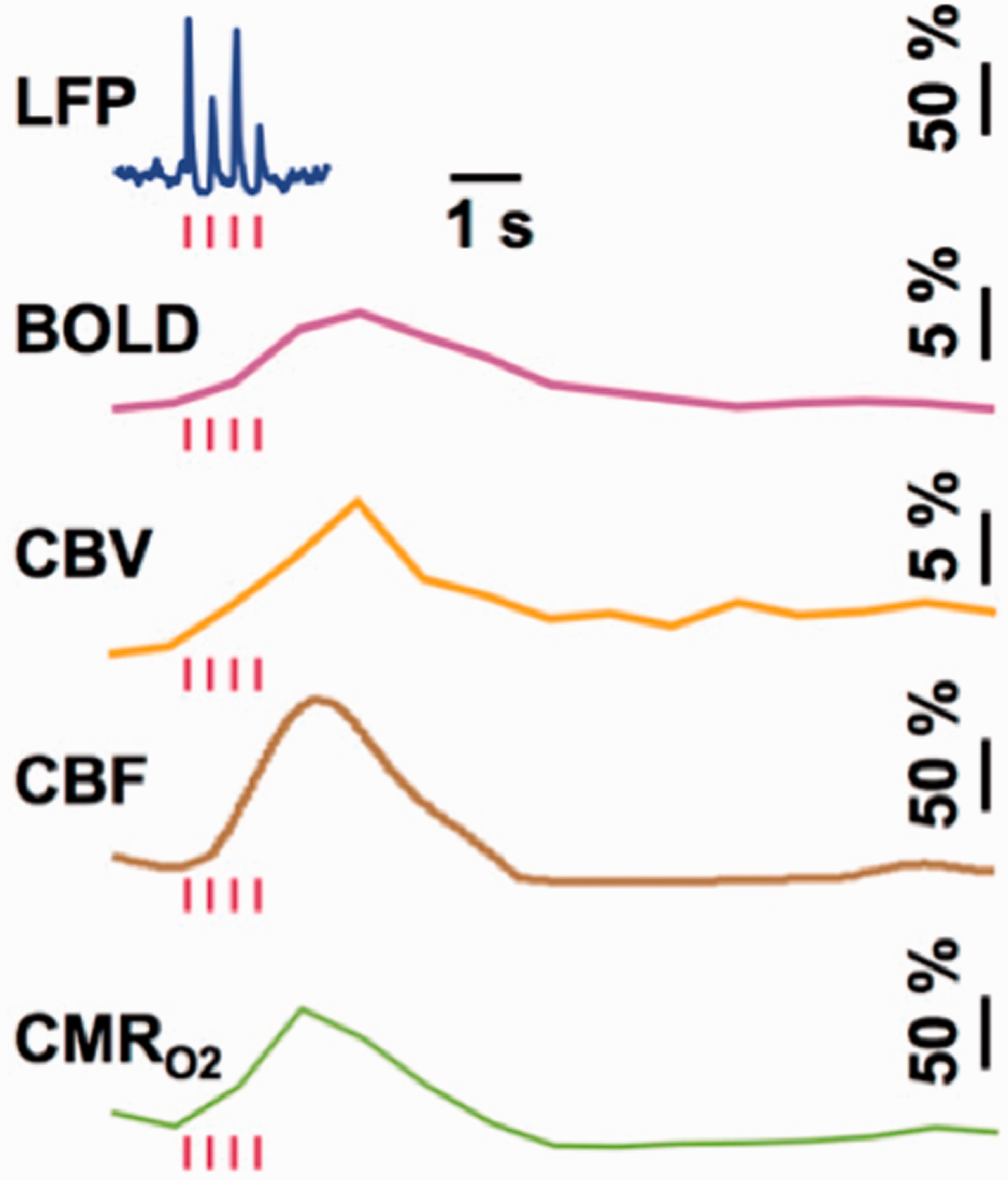
Single trial responses from rat cortex to sensory stimuli (red bars) showing LFP, BOLD, CBV, CBF, and CMR_O2 responses. From Herman et al (2009) J Neurochem ⁸³ with permission.

Interpretation of neural origins of the BOLD response is provisional on whether LFP and MUA, across brain regions, are disassociated or associated. ⁸² Logothetis and colleagues found that the sensory-evoked BOLD response in the primate cerebral cortex is better correlated to LFP than to MUA. ⁷² But this also implies that MUA is disassociated from LFP, and furthermore this type of neural-hemodynamic disassociation has been reported by others (see citations in ⁸² ). Both vascular-based and circuitry-based differences can cause regional dissociation between neural (MUA or LFP) and hemodynamic (BOLD or CBF) measurements. But do metabolic demands of neural-hemodynamic associated and disassociated areas in brain differ? To answer this question, results from two studies in rat brain examining sensory-evoked responses of BOLD, CBF, CBV, and CMR_O2 from rat’s ventral posterolateral thalamic nucleus (VPL) and cortical laminae of the somatosensory forelimb area (S1_FL) in relation to both MUA and LFP recordings^80,81 can be compared.

The rat’s VPL and S1_FL are two model brain regions where LFP and MUA can be associated or disassociated from the respective BOLD responses (Figure 2(a)). Since the capillary density in the thalamus and most cortical structures are quite similar, ⁸⁷ we expect the hemodynamic component to be comparable. However, the cellular morphology in these regions are dissimilar. The VPL consists of star-shaped thalamic cells such that the synaptic fields generated have potential to cancel out. ⁸⁸ In contrast, the pyramidal cells in S1_FL are oriented parallel along the cortex such that synaptic currents integrate and summate. ⁸⁸ In other words, generally the LFP should be much lower in VPL than in S1_FL. However, the upper, middle, and lower S1_FL segments are also quite different: the upper layer comprises of neurons projecting to other adjacent cortical areas, the middle layer includes inputs from the thalamus and projections to the spinal cord, and the lower layer has reciprocal connections to and from deeper brain regions.

Figure 2.

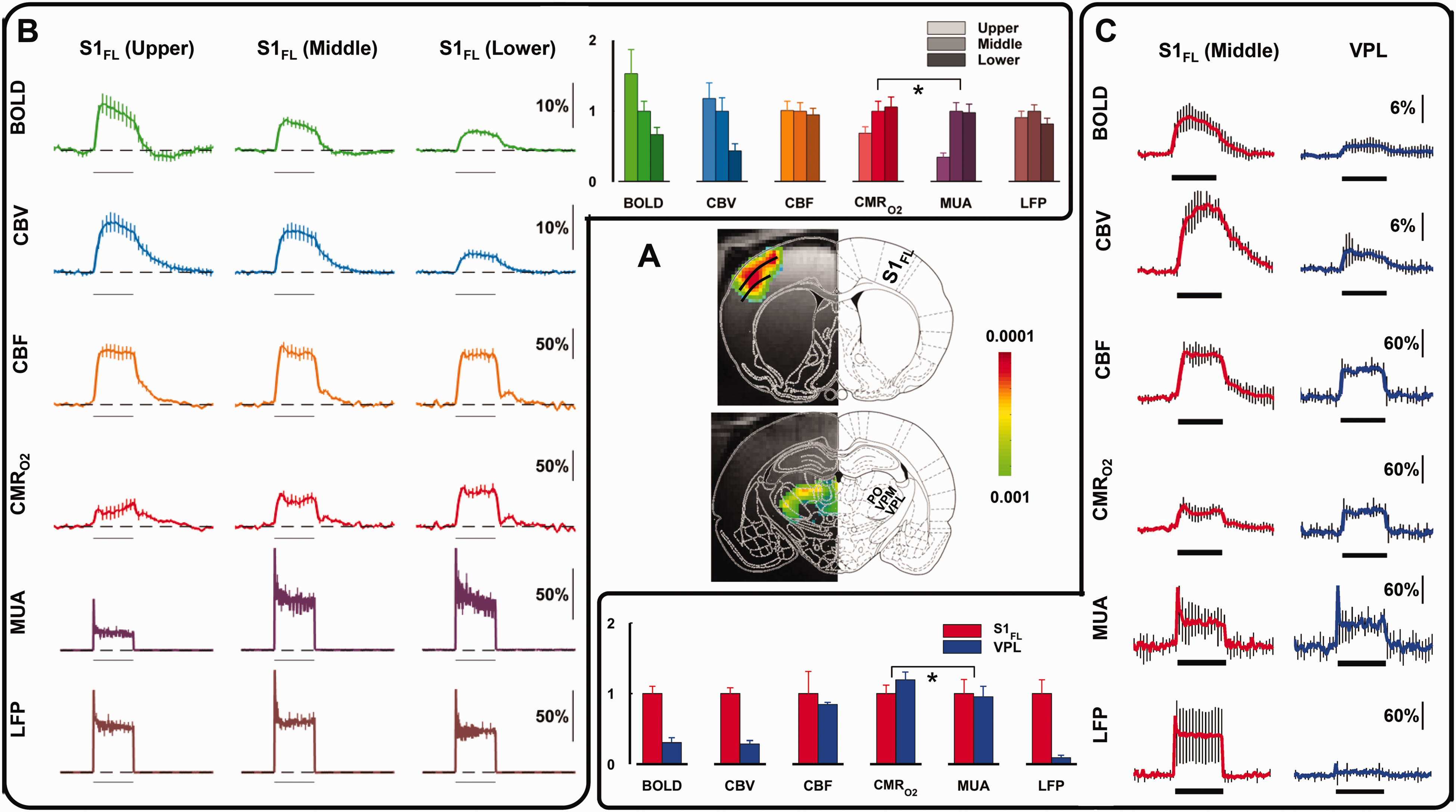
Calibrated fMRI derived metabolic changes in rat brain, comparison between activations in forelimb cortex (S1_FL) and thalamus separated into ventral posterolateral thalamic nucleus (VPL), ventral posteromedial nucleus (VPM), and posterior thalamic nuclear complex (PO) obtained during right forepaw stimulation (2 mA, 0.3 ms, 3 Hz) for 30 s (horizontal bar). (a) BOLD activation maps of S1_FL and VPL. From Sanganahalli BG et al (2016) J Cereb Blood Flow Metab. ⁸¹ (b) Multimodal responses of BOLD, CBV, CBF, CMRo₂, MUA, and LFP across cortical S1_FL laminae (upper, middle, and lower segments, each ∼600 μm thick). Horizontal bar represents 30 s of forepaw stimulation. (c) Multimodal responses of BOLD, CBV, CBF, CMRo₂, MUA, and LFP across cortical S1_FL middle laminae and VPL thalamic region. A and C are from Sanganahalli BG et al. (2016) JCBFM, ⁸¹ where B is from Herman P et al. (2013) Proc Natl Acad Sci USA. ⁸⁰

Layer-specific calibrated fMRI (BOLD, CBF, CBV, and CMR_O2) and electrophysiology (LFP, MUA) data in S1_FL during forepaw stimulation in the rat (Figure 2(b)) showed that BOLD and CBV responses were highest in superficial layers and lowest in the deepest layers, and these laminar trends did not correlate well with LFP or MUA responses.^80,81 In contrast, however, CBF and LFP responses were quite stable across all layers. Changes in CMR_O2 and MUA were varied across layers and were well correlated, lowest in the superficial layer and higher in the middle and deep layers. These animal results are similar to human calibrated fMRI findings of varied CBF-CMR_O2 coupling across brain regions (see review ⁸⁹ ) Comparison of calibrated fMRI and electrophysiology data in S1_FL (middle layer) and VPL during the forepaw stimulation (Figure 2(c)) showed that BOLD and CBV responses were greater in S1_FL than in VPL, and these hemodynamic changes were similar to LFP regional differences. However, CBF and CMR_O2 responses were both much larger and were comparable in S1_FL and VPL. Interestingly, despite different levels of CBF-CMR_O2 coupling and LFP-MUA coupling in both regions, the CMR_O2 was well matched with MUA in VPL and S1_FL.^80,81 These results suggest that neural-hemodynamic associated and dissociated areas can have similar metabolic demands, but this can only be revealed by comparing calibrated fMRI results.

The underpinnings for understanding the neuronal processes underlying BOLD contrast fMRI have largely been derived from animal studies, as such experiments are impossible to conduct in human subjects. However, most human calibrated fMRI studies are conducted in the awake state, while with animal models are executed under different types of anesthetics to achieve different levels of global brain activity.^90,91 The implications of these will be outlined in subsequent sections. Table 1 summarizes the biophysical relationship amongst all key variables for the BOLD contrast mechanism, irrespective of the calibration approach.

Table 1.

The calibrated fMRI model based on BOLD contrast.

Model building blocks	Equation
${\Delta R_2^{\mathrm{*}}=A·\mathit{CBV}·{\left[\mathit{dHb}\right]}^{\beta }-A·\mathit{CBV}}_0·{\left[\mathit{dHb}\right]}_0^{\beta }$	(1)
$\frac{\Delta \mathit{BOLD}}{{\mathit{BOLD}}_0}=e^{-TE·\Delta R_2^{\mathrm{*}}}\simeq =TE·\mathrm{\Delta }{R}_2^{\mathrm{*}}$	(2)
$M=TE{·A·\mathit{CBV}}_0·{\left[\mathit{dHb}\right]}_0^{\beta }$	(3a)
$M=TE\hspace{0.17em}·\hspace{0.17em}{R}_2^{\mathrm{\prime }}$	(3b)
$R_2^{\mathrm{\prime }}={A·\mathit{CBV}}_0·{\left[\mathit{dHb}\right]}_0^{\beta }$	(3c)
$\frac{\Delta \mathit{BOLD}}{{\mathit{BOLD}}_0}=M·\left(1-\frac{\mathit{CBV}}{{\mathit{CBV}}_0}·{\left(\frac{\left[\mathit{dHb}\right]}{{\left[\mathit{dHb}\right]}_0}\right)}^{\beta }\right)$	(4)
$\frac{\Delta \mathit{BOLD}}{{\mathit{BOLD}}_0}=M·\left(1-{\left(\frac{{\mathit{CMR}}_{O_2}}{{\mathit{CMR}}_{O_2,0}}\right)}^{\beta }·{\left(\frac{\mathit{CBV}}{{\mathit{CBV}}_0}\right)·\left(\frac{\mathit{CBF}}{{\mathit{CBF}}_0}\right)}^{-\beta }\right)$	(5)
${\frac{\mathit{CBV}}{{\mathit{CBV}}_0}=\left(\frac{\mathit{CBF}}{{\mathit{CBF}}_0}\right)}^{\alpha }$	(6)

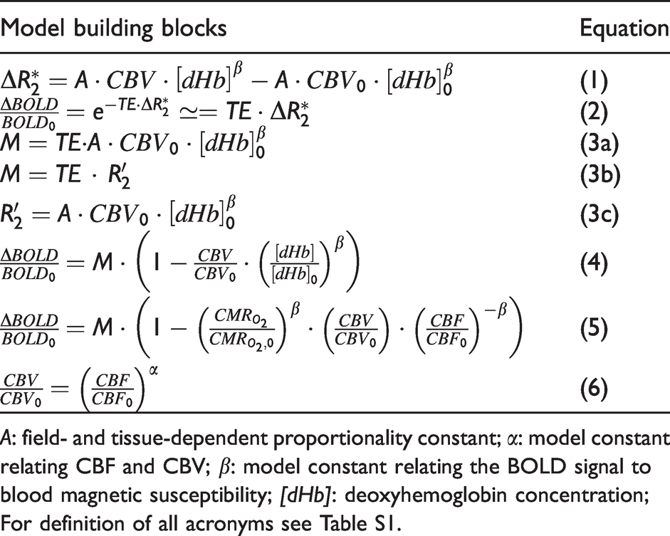
A: field- and tissue-dependent proportionality constant; $\alpha$ : model constant relating CBF and CBV; $\beta$ : model constant relating the BOLD signal to blood magnetic susceptibility; [dHb]: deoxyhemoglobin concentration; For definition of all acronyms see Table S1.

Calibrated fMRI using gas

The idea for calibrated fMRI rests on the assumption that it is possible to determine the maximum achievable BOLD signal intensity in tissue, which occurs when all deoxyhemoglobin (dHb) is eliminated from the vasculature (i.e., saturated by diamagnetic oxyhemoglobin). As it is impossible in reality to eliminate all dHb from the vasculature, calibrated fMRI with gas aims to manipulate the BOLD signal towards different conditions, thereby extrapolating the maximum BOLD signal change. Calibrated fMRI using inhaled gases has been thoroughly reviewed recently,^43,45,92 and will be reviewed here only briefly.

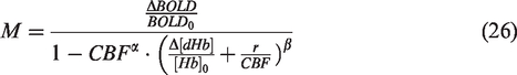
Since its introduction in 1998, ³⁸ the central focus of gas-calibrated fMRI has been to estimate the so-called “M-value” (see equations (1) to (6); Table 1). M represents the maximum achievable positive BOLD signal change, and it is field dependent. Given an accurate M, the CMR_O2 response amplitude (ΔCMR_O2) can be estimated from the CBF-CMR_O2 coupling ratio (n = ΔCMR_O2%/ΔCBF%) because the hemodynamic component, at least CBF (using ASL), is independently measured. Such a process also requires measurements of ΔCBF and ΔCBV. Given that CBV measurements have not been as accessible as those of CBF, it is customary in human studies to relate the CBF and CBV responses through a power-law relationship governed by the constant α (see equation (6); Table 1). Another important constant is β, which characterizes the relationship between deoxygenation-related field inhomogeneities in the reversible transverse relaxation rate (R₂′; Table 1).

Hypercapnia, hyperoxia, dual and generalized calibrated fMRI

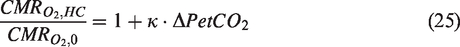
The gas perturbations are assumed to be physiologically benign. Table 2 (equations (7) to (16)) summarizes the systems of equations used in various calibrated fMRI to derive the “M-value”. It is evident from equation (5) that there are at least two unknowns, M and ΔCMR_O2. In the seminal work by Davis et al., ³⁸ hypercapnia was used as an iso-metabolic stimulus to simplify the calibrated fMRI equation (Table 1). As carbon dioxide presumably elicits CBF rise without altering CMR_O2, hypercapnic manipulation (within 5% CO₂) introduces a second BOLD (and CBF) measurement (in addition to that associated with neuronal activation) that allowed the two unknowns to be solved. In contrast, hyperoxic calibration ⁹³ relies on BOLD manipulations driven by intravascular dHb concentration ([dHb]). The goal remains the same – using the gas manipulation to generate two measurements to solve two unknowns. The key assumption, however, is that hyperoxia (ranging from 25% to 100% O₂) does not alter CBF. Both hypercapnic and hyperoxic calibration has been reviewed extensively in the literature,^{43,45,74,75,90,92,94} so the details will not be repeated here.

Table 2.

Summary of M-value estimation by different calibrated fMRI methods.

Method	Equation	Comments
Hypercapnic calibration 101 $M=\frac{\frac{\Delta \mathit{BOLD}}{{\mathit{BOLD}}_0}}{1-{\left(\frac{\mathit{CBF}}{{\mathit{CBF}}_0}\right)}^{\alpha -\beta }}$	(7)	Advantages: Well understood, robust CO2 response, can provide time-resolved CMRO2 response measurementCaveats: Lengthy set up, requirement for special equipment, unverifiable assumptions, potentially uncomfortable, contraindicated for chronic obstructive pulmonary disease
Hyperoxic calibration 184 $\frac{\Delta \mathit{BOLD}}{{\mathit{BOLD}}_0}=M·\left(1-\frac{\mathit{CBV}}{{\mathit{CBV}}_0}·{\left(\frac{\left[\mathit{dHb}\right]}{{\left[\mathit{dHb}\right]}_0}\right)}^{\beta }\right)$ $\hspace{1em}\frac{\left[\mathit{dHb}\right]}{{\left[\mathit{dHb}\right]}_0}=\frac{\varphi \cdot \left[Hb\right]\cdot \mathrm{\Delta }Y+\epsilon \cdot \mathrm{\Delta }{P}_a\cdot O_2}{\varphi \cdot \left[Hb\right]\cdot \left[1-\mathrm{\Delta }Y\cdot \left(1-\mathit{OEF}\right)\right]+\epsilon \cdot P_a\cdot O_2\cdot (1-\mathit{OEF})}$ $M=\frac{\frac{\Delta \mathit{BOLD}}{{\mathit{BOLD}}_0}}{1-{\left(\frac{\left[\mathit{dHb}\right]}{{\left[\mathit{dHb}\right]}_0}\right)}^{\beta }}$	(8)(9)(10)	Advantages: More comfortable, can provide time-resolved CMRO2 response measurementCaveats: Lengthy set up, requirement for special equipment, unverifiable assumptions $\varphi$ : oxygen carrying capacity of hemoglobin $\Delta Y$ : change in blood oxygenation $\Delta P_a$ : change in arterial oxygen tension $O_2$ : oxygen saturation of arterial hemoglobin $\epsilon$ : solubility coefficient of oxygen in blood
Dual calibration 96 $M=\frac{\frac{\Delta \mathit{BOLD}}{{\mathit{BOLD}}_0}}{1-{\left(\frac{\mathit{CBF}}{{\mathit{CBF}}_0}\right)}^{\alpha }·{\left(\frac{\left[\mathit{dHb}\right]}{{\left[\mathit{dHb}\right]}_0}\right)}^{\beta }}$ ${\mathit{CMR}}_{O_2}=C_a{O}_2·\mathit{OEF}·\mathit{CBF}$	(11) (12)	Advantages: Builds upon well-understood signal models, can provide time-resolved CMRO2 response measurement, can also provide baseline CMRO2Caveats: Lengthy set up, requirement for special equipment, unverifiable assumptions, CO2-related caveats $C_a{O}_2$ : arterial oxygen concentration
Gas-free: T2-based calibration 112 $M=TE{·A·\mathit{CBV}}_0·{\left[\mathit{dHb}\right]}_0^{\beta }=TE·A{·\mathit{CBF}}_0^{\alpha }·{\mathit{Hct}}^{\beta }·{(1-Y_{v,0})}^{\hspace{0.17em}}$	(13)	Advantages: Methods is simple, with relatively high SNR. Caveats: T2 is only measured in a large vein, not accounting for spatial heterogeneity.  Yv,0: baseline venous oxygenation
Gas-free: R2′-based calibration 40 $M=TE{·A·\mathit{CBV}}_0·{\left[\mathit{dHb}\right]}_0^{\beta }=TE·R_2^{\mathrm{\prime }}$ $R_2^{\mathrm{\prime }}=A·\mathit{CBV}·{\left[\mathit{dHb}\right]}^{\beta }$ $R_2^{\mathrm{\prime }}=R_2^{\mathrm{*}}-R_2^{}$	(14) (15) (16)	Advantages: No need for any gas or breathing challengeCaveats: Relies on accurate estimation of R2′ and β.

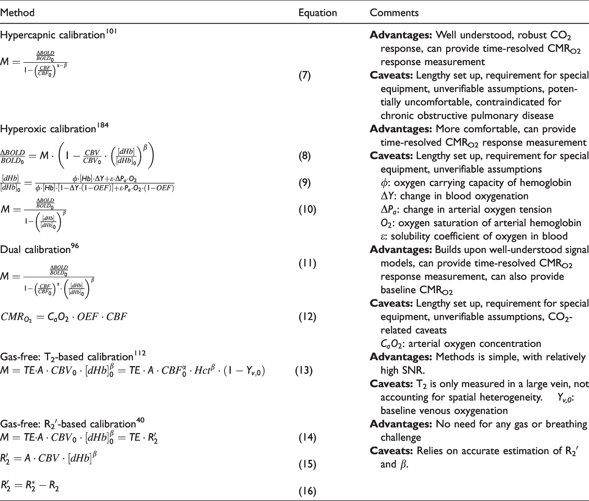
Dual-gas calibrated fMRI methods were introduced to quantitatively measure the baseline oxygen extraction fraction (OEF).^95–97 This more complicated setup relies on two types of respiratory challenges (hypercapnia and hyperoxia) to produce changes in the BOLD signal, along with similar measurements as described above for single gas (either CO₂ or O₂) calibrated fMRI. The generalized calibrated fMRI model was later presented by Gauthier and Hoge. ⁹⁸ Using this model, it is not necessary for hyperoxia to be iso-capnic (or for that matter, for hypercapnia to be iso-oxic). Hyperoxic data is used to produce the functional relationship between M and the resting OEF₀, while the hypercapnic data provides another relationship between M and OEF₀. The use of these two relationships produces solutions for the two unknowns M and OEF₀. The model is valid for arbitrary combinations of CBF and oxygenation changes. A more recent specific variant of the generalized calibrated fMRI model, known as QUantitative O2 (QUO2) MRI,^99,100 involves the use of three gases to produce three conditions, namely hypercapnia, hyperoxia and hypercapnic-hyperoxia. The mean CBF and BOLD percent changes as well as the measured end-tidal partial pressure of oxygen (PetO₂) are fed to the generalized calibration model, and a constant hyperoxia-induced CBF reduction is assumed.

It should be noted that the calibrated BOLD signal model proposed by Davis et al. ³⁸ (and adapted by Hoge et al. ¹⁰¹ ) is fundamentally empirical. That is, the relationships between CBF and CMR_O2, between CBF and CBV, and between BOLD and the M variable are derived from ad hoc fits to experimental data. While the functional form of the BOLD model may be able to fit many types of BOLD data, it remains difficult to substantially enhance the precision of calibrated fMRI parameters. This is a major ongoing challenge for the field.

Variability in the M value

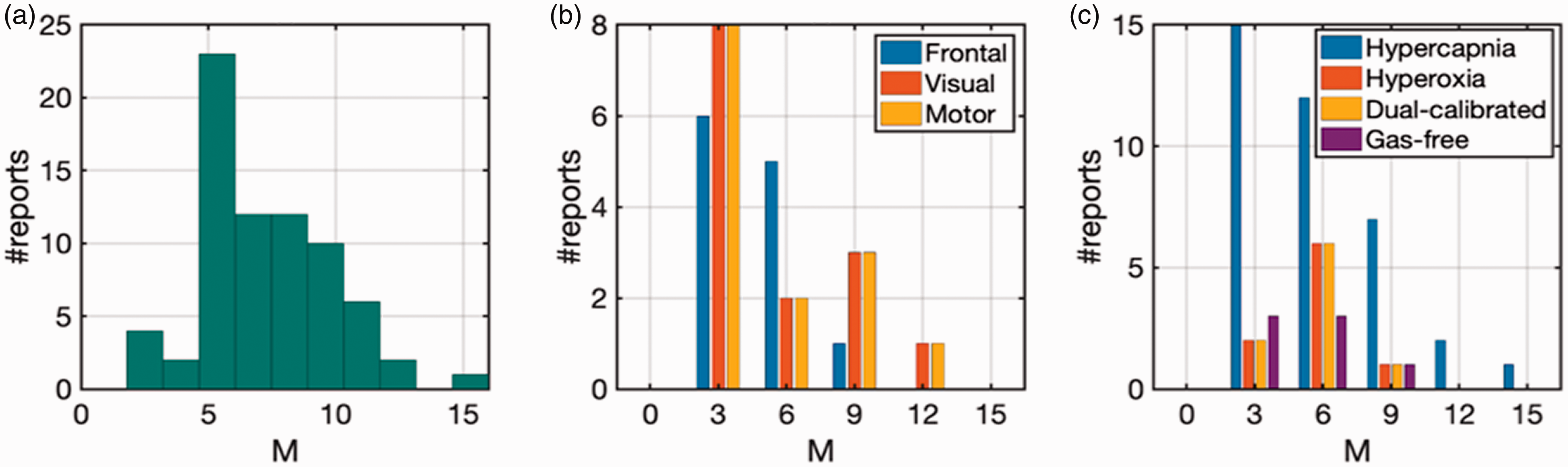
Gas calibration is an empirical approach as opposed to a first-principles-driven approach, and the estimation of the maximum achievable BOLD signal relies on our ability to accurately estimate the asymptotic BOLD value using two data points in the linear range. As recently summarized, ¹⁰² a very wide range of M-values has been reported in animal and human calibrated fMRI experiments. In this work, we focus on human studies, and the large variability of M estimates due to various factors amongst human studies is summarized in Figure 3, with the details provided in Table S2. Related biases in gas calibrated fMRI have also been simulated in detail previously,^94,103 and will not be repeated here.

Figure 3.

Summary of calibrated BOLD results from human 3 T experiments from 2009 to 2020.^{45,98,161,184,222} Reported M values from (a) all studies, (b) specific to frontal, visual, and motor cortices, and (c) derived from different gas preparations. See Table S2 for details.

A fundamental limitation in gas-based calibrated fMRI is the over-reliance of accurate M-value estimation on a single gas-driven step. It should be noted that the experimental data obtained for BOLD and CBF changes during the gas exposures represent a very small portion of the pseudo-linear relation of a highly non-linear CBF-BOLD relationship. The measured CBF increases during gas exposure are less than 10–20%,^38,96 whereas the exponential fitting that defines the M-value from the asymptotic limit for BOLD signal change is only reached when CBF increases are a fold or two higher,^98,101 and it is difficult to reach such large CBF changes safely in humans.^104–109 Thus, small experimental errors in BOLD or CBF measurements can substantially bias the M-value derived from asymptotic fitting. ¹⁰² This point is demonstrated by the fact that the M estimate depends on the optimal TE, which is field-strength dependent. ¹¹⁰

Moreover, as shown in Table 2, the high variability of M-value estimation could also be caused by differences in calibration approaches and their associated assumptions (see equation (7) vs. equations (8) to (10) vs. (11) and (12) vs. (13) vs. (14) to (16)). Blockley et al. measured M-values by two different methods in the human cerebral cortex: hypercapnia challenge and the R₂′ method (which will be discussed later). They found small differences in M-values between visual cortex and the whole grey matter with the R₂′ method, but regional variations in M-values were significantly higher with the hypercapnia challenge. Their study, in agreement with the observations by Shu et al. in the rat brain, ¹⁰² suggests that degree of regional M variations depends on the calibration method. The high variability in M-value has also been attributed to BOLD and CBF responses being calculated in separate steps. ¹¹¹ Gas-free calibration, in contrast to gas-based calibration, does not rely on physiological assumptions, and may be an increasingly feasible approach for the eventual consolidation of calibrated fMRI findings.

Gas-free calibration

In gas-free conditions, OEF, hence [dHb] in the resting state, is estimated through intravascular transverse relaxation time (T₂) relaxometry, ¹¹² T2-oxygenation modeling ¹¹³ or venous susceptometry. ¹¹³ Specifically, these methods provide an estimate of global OEF, which has been demonstrated as uniform across the cortex. ¹¹⁵ However, in this review, we will focus on voxel-wise calibration methods for determining [dHb] to allow spatial mapping of OEF.

R2’-based calibration

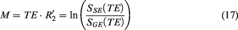
It has long been known that the reversible transverse relaxation rate, R₂′, is sensitive to venous cerebral blood volume (CBVv) and the concentration of deoxyhemoglobin ([dHb]). ¹¹⁶ These are the same entities that define the M-value, for what is “M” but the product of echo time (TE) used in the calibrated fMRI experiment and R₂′ (see Table 1). Thus, the M- value can be determined from the baseline R₂′ under well shimmed conditions. The use of R₂′ mapping for estimating CMR_O2 has been demonstrated in rat, mouse, and human brain calibrated fMRI studies.^41,117–120

More recently, following the proposal of the quantitative BOLD (qBOLD) method ¹²¹ the feasibility of gas-free T2’ calibration has been revisited.^94,122 The Yablonskiy-Haacke model of T₂′ (inverse of R₂′) dependence on vascular physiology offers the potential to simultaneously yet non-invasively quantify blood oxygenation saturation (SO₂) and CBV.^116,121,123 A summary of the various approaches to R₂′ estimation is provided in Table 3.

Table 3.

Methods to map R₂’.

Method	Comments
GE-SE	Advantages: Simple to implement and analyze; low power deposition. Caveats: GE and SE acquired separately, effects such as ΔB0 and slice positioning may change between scans; isolation of R2 from R2* effects difficult at longer TEs.
ASE	Advantages: Low power deposition; low time consumption; matched ΔB0 and slice positioning between all echoes. Caveats: Limited number of samples along decay curve; isolation of R2 from R2* effects difficult at longer echo shifts.
GESFIDE	Advantages: Low power deposition; availability of numerous samples along the dephasing and rephasing curves. Caveats: Higher time consumption; sensitive to refocusing efficiency.
GESSE	Advantages: Low power deposition; availability of numerous samples along decay curve; insensitive to refocusing efficiencyCaveats: Higher time consumption; lower SNR than GESFIDE.
GESEPI	Advantages: Based on EPI, so low time consumption; low power deposition. Caveats: Image distortion due to EPI readout.
EPTI	Advantages: Highest temporal and spatial resolution of all available methods; availability of extremely high sampling of the dephasing and rephasing curves. Caveats: Sensitive to movement, due to simultaneous multi-slice reconstruction of down-sampled k-space; inter-echo spacing tied to spatial resolution, difficult to customize.
MRF	Advantages: Highest versatility in acquisition parameters of all available methods; high spatial resolution. Caveats: Randomization of sampling locations along the dephasing curve, difficult to customize for R2′ sensitivity to vasculature.

Separate gradient- and spin-echo based methods

The easiest way to map R₂′ is from independent R₂ and R₂* maps measured using gradient-echo (GE) and spin-echo (SE) EPI acquisitions, respectively. The principle of using an SE experiment to remove extravascular BOLD effects relies on the assumption that the majority of the BOLD effect emanates from the extravascular compartment. Several studies have used separate GE and SE acquisitions to obtain R₂′ maps,^{102,120,124,125} in which M can be expressed as ⁹⁴

$$M=TE·R_2^{\mathrm{\prime }}=\ln \left(\frac{S_{SE}\left(TE\right)}{S_{GE}\left(TE\right)}\right)$$

(17)

where S_SE and S_GE are the SE and GE signals, respectively. A key consideration in such an approach is co-registration of the GE and SE images. Dynamic processes including head-motion, respiration and even heart beats can lead to mismatches between the GE and SE signals for a given voxel. In addition, stimulated echoes due to the use of multiple refocusing pulses can lead to R₂ underestimation. Stimulated echoes most commonly arise from imperfect matching between excitation and refocusing pulse profiles in 2D image acquisitions or static magnetic field inhomogeneities (ΔB₀).^126,127 To enable whole-brain acquisitions in a reasonable amount of time, 3D imaging using non-selective RF pulses has been proposed. ¹²⁸ To combat stimulated echoes, more elaborate pulse cycling schemes ¹²⁹ can be employed, but at the cost of increased acquisition time. Nonetheless, the efficacy of phase cycling in regions of large ΔB₀ remains low. ¹³⁰ In addition to separately measuring R₂* and R₂ to find R₂′, other methods have been developed in the past to measure R₂′ in a single scan.^131–134 However, the implementation of these R₂′ mapping methods for calibrated fMRI scans remains unexplored.

Combined gradient- and spin-echo based methods

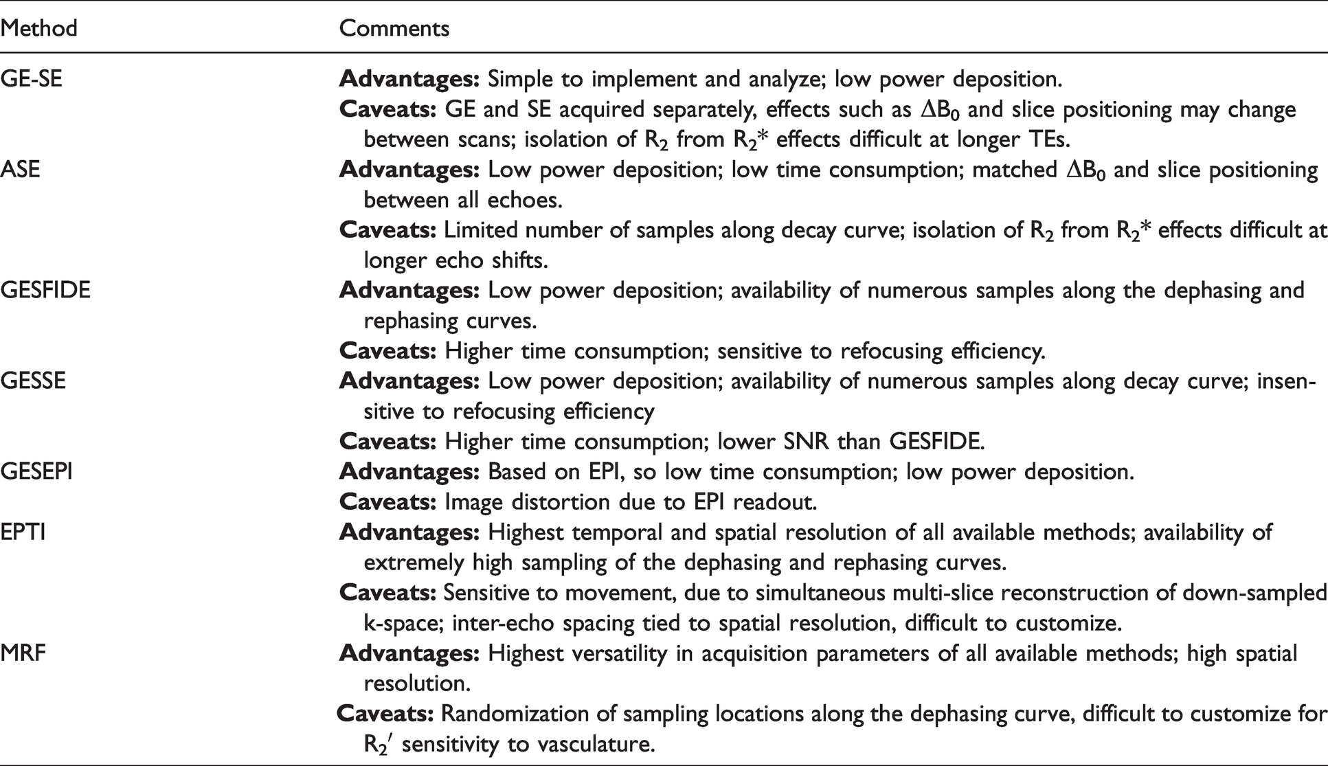
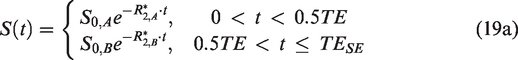
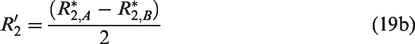
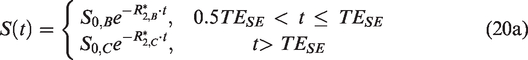
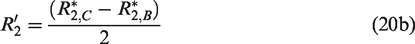
Combined GE-SE methods have become dominant in quantitative BOLD research. These methods include gradient-echo sampling of spin-echo (GESSE), gradient-echo sampling of free induction decay and echo (GESFIDE) and asymmetric spin echo (ASE)^135,136 which all use a single spin-echo (instead of multiple spin-echoes as in the previous section) to quantify T₂ (see Figure 4).

Figure 4.

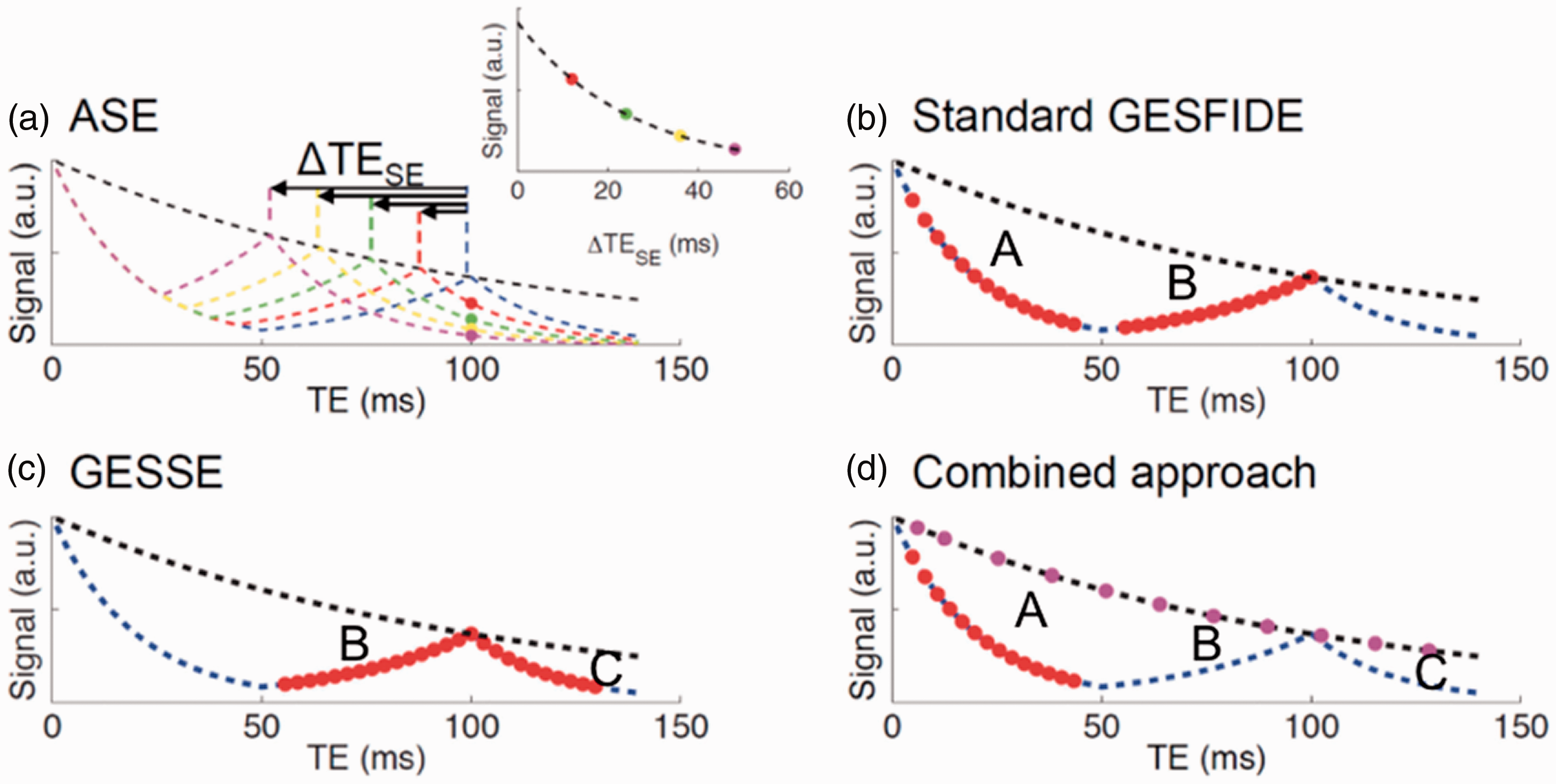
TE dependence of asymmetric spin echo (ASE), gradient-echo sampling of free-induction decay and echo (GESFIDE), gradient-echo sampling of the spin echo (GESSE), and combined approach shown in a-d respectively. Figure is modified from ¹³⁵ with permission.

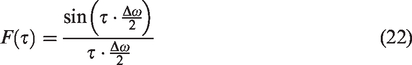
ASE with EPI is the most intuitive way to measure R₂′. ¹³³ In the ASE acquisition (Figure 4(a)), the refocusing pulse is shifted by τ/2, and the signal (S_ASE) is acquired at TE, whereas the spin echo forms at TE-τ.

$$S_{\mathit{ASE}}=S_0{e}^{-TE·R_2}·e^{-t·R_2^{\mathrm{\prime }}}·F\left(\tau \right)$$

(18)

where F is the attenuation factor due to the shift τ from the spin-echo time. Using a series of different τ values, R₂′ can be directly obtained from the ASE signal. Since ASE is most commonly based on conventional SE-EPI, it is unable to perfectly refocus the spin-echo due to susceptibility effects. Thus, ASE underestimates R₂′, and hence M in a manner that depends on TE, ASE offset and vessel size. Specifically, imperfect SE refocusing from diffusion of water near microvasculature. ¹³³ Another cause for M overestimation is inhomogeneities near air-tissue boundaries leading to loss in EPI quality.

The GESFIDE technique ¹³² (Figure 4(b)) involves sampling of the period starting immediately after the excitation pulse, spanning the free-induction decay (FID, t < 0.5TE) and rephrasing (t > 0.5TE), and ending at the centre of the spin-echo. R₂′ is estimated from the FID and refocusing pulse as follows.

$$S\left(t\right)=\left\{\begin{array}{cc}{S}_{0,A}{e}^{-R_{2,A}^{\mathrm{*}}·t},& 0<t<0.5TE\\ S_{0,B}{e}^{-R_{2,B}^{\mathrm{*}}·t},& 0.5TE<t\le {TE}_{SE}\end{array}\right.$$

(19a)

$$R_2^{\mathrm{\prime }}=\frac{(R_{2,A}^{\mathrm{*}}-R_{2,B}^{\mathrm{*}})}{2}$$

(19b)

where τ represents the duration between the given sampling time and the spin-echo time. GESFIDE’s application in R₂ and R₂′ quantification was compared to that of a Carr-Purcel Meiboon-Gill multi-echo spin-echo technique. ¹¹⁹

The GESSE technique ¹³⁴ derives from GESFIDE (Figure 4(c)), which shifts the sampling window to the rephasing stage, the spin-echo, and the dephasing stage. The rationale is that the signal segments flanking the spin-echo would be equally affected RF pulse profile imperfections in the refocusing pulse, resulting in less R₂′ bias. However, the cost is signal-to-noise ratio (SNR), as the signal intensity would be lower than that of GESFIDE.

$$S\left(t\right)=\left\{\begin{array}{cc}{S}_{0,B}{e}^{-R_{2,B}^{\mathrm{*}}·t},& 0.5{TE}_{SE}<t\le {TE}_{SE}\\ S_{0,C}{e}^{-R_{2,C}^{\mathrm{*}}·t},& t{>TE}_{SE}\end{array}\right.$$

(20a)

$$R_2^{\mathrm{\prime }}=\frac{(R_{2,C}^{\mathrm{*}}-R_{2,B}^{\mathrm{*}})}{2}$$

(20b)

A natural extension, proposed by Ni et al., ¹³⁵ is to combine GESFIDE and GESSE and compute R₂′ from the FID, rephrasing and second-dephasing segments (Figure 4(d)). That is,

$$S_{R_2^{\mathrm{*}}}\left(t\right)=S_{{0,R}_2^{\mathrm{*}}}{e}^{-R_2^{\mathrm{*}}·t},\mathrm{ }0<t<0.5{TE}_{SE}$$

(21a)

$$S_{R_2^{}}\left(t\right)=S_{{0,R}_2^{}}{e}^{-R_2^{}·t},\mathrm{ }t>0$$

(21b)

$$R_2^{\mathrm{\prime }}=R_2^{\mathrm{*}}-R_2^{}$$

(21c)

A comparison of ASE, GESFIDE and GESSE for R₂′ mapping has been reported in detail. ¹³⁵ All of these methods suffer from underestimation of R₂ (and thus overestimation of R₂′) due to intravoxel through-plane dephasing. The attenuation can be described as

$$F\left(\tau \right)=\frac{\sin (\tau ·\frac{\mathrm{\Delta }\omega }{2})}{\tau ·\frac{\mathrm{\Delta }\omega }{2}}$$

(22)

where Δω is the frequency difference across the voxel. This is a function of the slice-select gradient and the slice thickness. In regions with pronounced susceptibility gradients (e.g. air-tissue interfaces), the effect is magnified. Thus, Blockley et al. introduced the use of thin-slice EPI acquisition to minimize R₂* effects in R₂ measurements. ¹³⁷ Simon et al. used two pairs of GESSE image series, one an early SE series (e.g. TE₁ = 48 ms) and one a late SE series (e.g. TE₂ = 98 ms), ¹³⁸ each sampled at 0.63 ms spacing to produce 2 series of 64 samples. From these (S(t)), R₂′ is estimated as

$$R_2^{\mathrm{\prime }}=\frac{1}{2}\left[\frac{d{\ln \left(S\left(t\right)\right)}_{TE2}}{dt}-\frac{{d\ln \left(S\left(t\right)\right)}_{TE2}}{dt}\right]$$

(23)

It is expected within these two spin-echoes, that R₂′ and ΔR₂* are similarly sensitive to variation in the baseline hematocrit, venous blood oxygenation and venous CBV but yet they are differentially sensitive to variation BOLD-related parameters. ¹³⁸

Analogous to GESFIDE is gradient-spin-echo (GE-SE) echo-planar time-resolved imaging (EPTI), ¹³⁹ in that it samples the refocusing and spin-echo portions of the T₂ decay curve. It uses a hybrid k-time space in conjunction with slice-acceleration and multiple shots to sample a 3D k-space, and assumes small variations in RF coil-sensitivity profiles to inform the reconstruction kernel. It is able to achieve an inter-echo interval of 1 ms and a spatial resolution of 1.1 × 1.1 × 3 mm within 30 sec. Moreover, GE-SE EPTI has demonstrated robustness against ΔB₀, as B₀ effects are intrinsically corrected in the reconstruction process. However, there is residual R₂* effect in the spin-echoes due to the interpolative nature of EPTI. This is nonetheless limited to a kernel full-width-at-half-minimum of ∼7 ms. ¹⁴⁰ The high SNR and sampling rate of EPTI may make it an attractive alternative for R₂′ mapping.

Magnetic resonance fingerprinting

Magnetic resonance fingerprinting (MRF) has been represented as a novel and versatile relaxometry technique, although most MRF studies have been concerned with estimating longitudinal (T₁) and transverse (T₂) relaxation times. More recently some effort has been put into estimating T₂* (i.e., inverse of R₂*) along with T₁ and T₂. The three published studies in this regard, which are all based on spiral readouts, have relied on a variable TE, ¹⁴¹ a combination of steady-state free precession (SSFP) with GE acquisition ¹⁴² or balanced SSFP (bSSFP) with RF phase variations. ¹⁴³ The latter allows the separation between intravoxel dephasing and B₀ offsets (two aspects of T₂′), and can, in theory, be useful for quantitative fMRI. However, despite the dominance of spiral-based MRF methods, it should be recognized that spiral MRI is very sensitive to errors in gradient fields, leading to the need for more complex off-line reconstruction; this presents a nontrivial implementation challenge across different sites. Recently, EPI-based MRF methods ¹⁴⁴ have been proposed that can quantify R₂*. Such methods encapsulate the TE-dependence of R₂* into a single R₂* estimate, but are still sensitive to B₀-dephasing effects, as is expected. As we are interested in the intravoxel frequency distribution underlying R₂′ more than we are interested in the R₂′ itself, MRF R₂′ mapping methods need to minimize the macroscopic ΔB₀ contribution. Moreover, it is important to remember that R₂* and R₂′ in fMRI are technique-specific, and it is still unclear how the R₂* and R₂ values estimated by MRF can be used to derive brain physiology.

Variability in estimates

Irrespective of the measurement technique, at lower fields there is a significant relaxation component from the intravascular compartment, which could induce some multi-exponential behaviours that are amplified at lower spatial resolution. These behaviours, in theory, bias R₂′ estimates irrespective of the method used. At 9.4 T, Shu et al. benefited from high magnetic field strength with its inherent higher spatial resolution and reduced intravascular weighting to achieve mono-exponential R₂′ decay.^102,125 Under these experimental conditions, R₂′ (and β) should in theory not vary significantly between R₂′ methods, but further measurements are needed to confirm this observation.

Moreover, while it may seem technically straightforward to measure a value of R₂′, the interpretation of R₂′ in calibrated fMRI depends on a large number of modeling parameters that describe the architecture of the tissue vasculature. R₂′ calibration schemes are sensitive to unmeasured model parameters describing CBV-CBF coupling, vascular size and orientation, as well as blood-tissue iso-susceptibility oxygenation, baseline hematocrit, oxygenation and volume of the deoxygenated compartment. ¹⁴⁵ Furthermore, different R₂/R₂* methods, as detailed in the following, will result in different R₂′ estimates, as described earlier. A main contributor to this variability is residual macroscopic ΔB₀, which could result from poor shimming and incomplete refocusing.^41,102 The variability in estimates can be gleaned from Table S3, and we also discuss these contributing factors in more detail in the following subsections. We also note that currently, calibrated fMRI is only performed in the grey matter. The white matter fMRI signal is low due to the limited blood supply, and can also be influenced by alterations in myelin susceptibility and iron content.

Applications in disease

Pathological conditions can challenge many of the long-standing assumptions in calibrated fMRI, and in broadening the applications of gas-based calibrated fMRI, it is important to design experiments that are robust against these uncertainties. Gas-free calibration harkens to a more quantitative approach to calibrated fMRI, by appropriately integrating a more complex biophysical model of the vasculature based on past modeling works.^{121,138,146,147} At the time of this review, we believe examples of calibrated fMRI, specifically with gas-free approaches, are on the verge of being applied more widely. Some cases of applications are given below.

So far the largest group study that uses gas-calibrated fMRI among patients is by Lajoie et al. from the Hoge group in Montreal, Canada, ¹⁴⁸ amongst 37 mild-moderate Alzheimer’s patients. CBF was measured using pseudo-continuous ASL, whereas OEF and CMR_O2 are estimated using the comprehensive calibrated BOLD technique. CMR_O2 deficits are found to be more widespread than those in CBF and OEF, reduced in the parietotemporal and precuneus regions, consistent with nuclear-medicine findings. ¹⁴⁹ More recently, to assess if there are alterations in CBF-CMR_O2 uncoupling in one side of the brain, patients with asymptomatic unilateral carotid artery stenosis were studied juxtaposed with normal age-matched controls by the Preibisch group in Munich, Germany. ¹⁵⁰ They used gas-free calibrated fMRI, but to raise the precision they included an independent CBV measurement using contrast agent injection. Figure 5(a) shows that while the R₂′, CBV, OEF or CBF maps look similar between control and patients, the CMR_O2 maps can reveal subtle differences attributed to the mild pathology. Moreover, the CBF-CMR_O2 couplings for each hemisphere within control (Figure 5(b)) and stenosis (Figure 5(c)) subjects clearly reveal CBF-CMR_O2 uncoupling on the side with stenosis. Similarly, to assess if there are variations in metabolism with concussion, the Cook group from Queens University, Canada used gas-calibrated fMRI. ¹⁵¹ They studied normal college students and athletes who had suffered concussion. Using standard procedures for M-value estimation using hypercapnia challenges, their subject-specific data of M, CBF, and CMR_O2 (Figure 5(d)) showed that the CMR_O2 was significantly reduced in concussion patients (Figure 5(e)) in a manner similar to the CBF reduction in their brains. In other words, the CBF-CMR_O2 couplings in students with and without concussion were not different, but their basal rates of flow and metabolism were dramatically altered.

Figure 5.

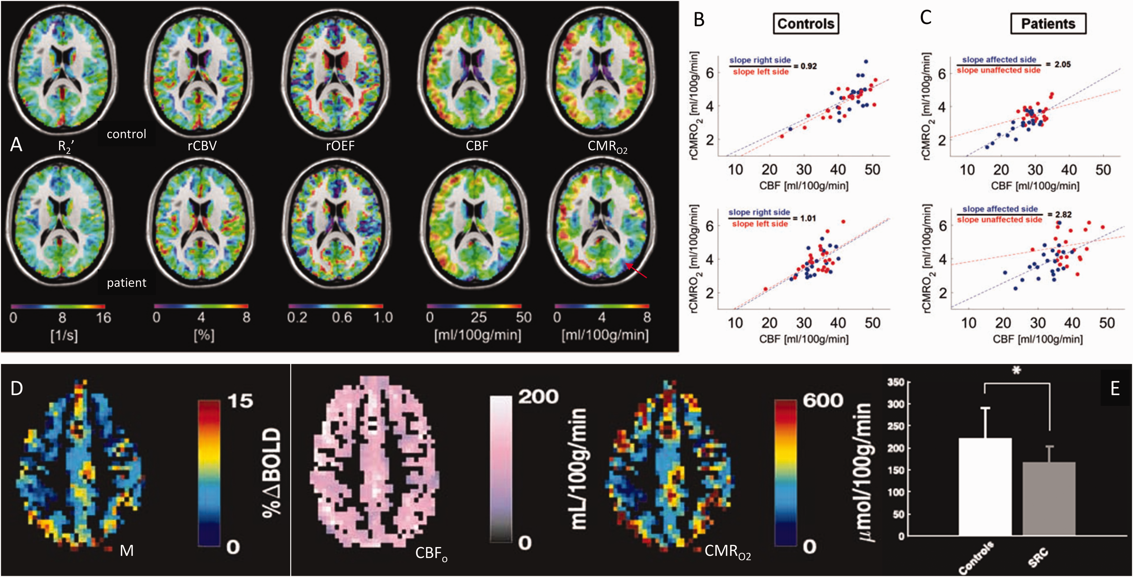
Calibrated fMRI in clinical scenarios at 3.0 T. (a) Multi-parametric maps of R₂′, CBV, OEF, CBF and CMR_O2 from a control subject (top row) and a patient with asymptomatic unilateral carotid artery stenosis (bottom row). The red arrow on the CMR_O2 map of the patient shows the subtle change in metabolism in the left side of the brain, which is not clearly reflected in the other maps. (b,c) Interhemispheric flow-metabolism coupling is shown across gray matter areas in the left (red dots) and right (blue dots) hemispheres in (b) two control subjects and (c) two patients with asymptomatic unilateral carotid artery stenosis. The left side of the brain in patients clearly have an abnormal flow-metabolism coupling. (d) Demonstration of M, CBF, and CMR_O2 maps of control subjects using gas-challenge calibrated fMRI. (e) CMR_O2 was significantly reduced in sport-related concussion (SRC) group compared to controls. This drop in CMR_O2 was similar to the CBF drop in the SRC group. (a–c) are from Figures 2 and 5 in ¹⁵⁰ with permission. (d,e) are from Figures 2 and 5 in ¹⁵¹ with permission.

Remaining issues and potential solutions

Field inhomogeneity effects

As mentioned earlier, accounting for ΔB₀ effects remain a challenge for R₂′-weighted experiments. Early methods for correction of B₀ effects in larger thickness than in-plane dimensions assumed that the B₀ variation across a voxel is approximately linear. ¹⁵² One recent solution has been to decrease the slice thickness in 2D acquisitions. Specifically, the GESEPI (gradient-echo slice excitation profile imaging) technique ¹³⁷ uses thin-sliced ASE EPI to circumvent the B₀-related T₂* effects. Liu et al. ¹⁵³ used thin-sliced GESSE to the same end, in addition to using FLAIR to minimize cerebrospinal fluid (CSF)-related B₀ inhomogeneity. Alternatively, He and Yablonskiy assumed that B₀ effects have low spatial frequency, and regressed low-frequency harmonics out of the GESFIDE images. ¹²¹ However, neither of these approaches are likely to withstand severe B₀ inhomogneities, such as found in the medial temporal/orbitofrontal lobes or at ultra-high field. Acquisition of a separate B₀ map for B₀ correction seems the most viable option in such cases.

Partial-volume effects in R2′

R₂′ estimates are highly sensitive to MRI signal contamination by CSF, irrespective of the method used. On the one hand, the long T₂ of CSF is likely not accurately captured by the range of TEs used in the methods described herein. Perhaps a less obvious source of bias is signal dephasing resulting from a small amount of CSF mixed with parenchyma. Dickson et al. estimated the off-resonance frequency resulting from dephasing due to partial-volumed CSF with 4% grey matter to be approximately 7 Hz. ¹⁵⁴ Such dephasing would contribute to R₂′. This is likened to a chemical-shift effect, and tends to cause M overestimation. These issues are relevant to GE-SE and MRF methods alike. To address this, fluid attenuation has been proposed, ¹⁵⁵ with the caveat that fast flowing CSF cannot be suppressed. Simon et al. proposed to incorporate a CSF compartment when computing R₂′, as well as use fluid-attenuated (FLAIR)-GESSE to minimize the contribution of CSF-related B₀ inhomogeneities.^138,153 On the other hand, it is desirable to achieve higher spatial resolution in order to avoid partial-volume effects. In that regard, EPTI and MRF-based methods, with their smaller voxels, represent promising options.

TE dependence of R2′

The R₂′ value depends on the method of measurement, as discussed earlier. Moreover, the grey matter contains multiple T₂ species (i.e. blood vessels, iron, etc) and additional diffusion processes that could lead to multiexponential T₂ decay. It is hence little surprise that R₂′ is found to increase with decreasing TE_SE, at least in the GESSE sequence. ¹³⁵ In response, the use of two GESSE imaging sequences with different spin-echo times has been proposed, ¹³⁸ as described earlier.

Vascular dependence of R2′

The calibrated fMRI models, whether gas-based or gas-free, all make certain assumptions about the composition of the voxels of interest. A summary of the cerebrovascular factors and assumptions affecting R₂′ are shown in Figure 6.

Figure 6.

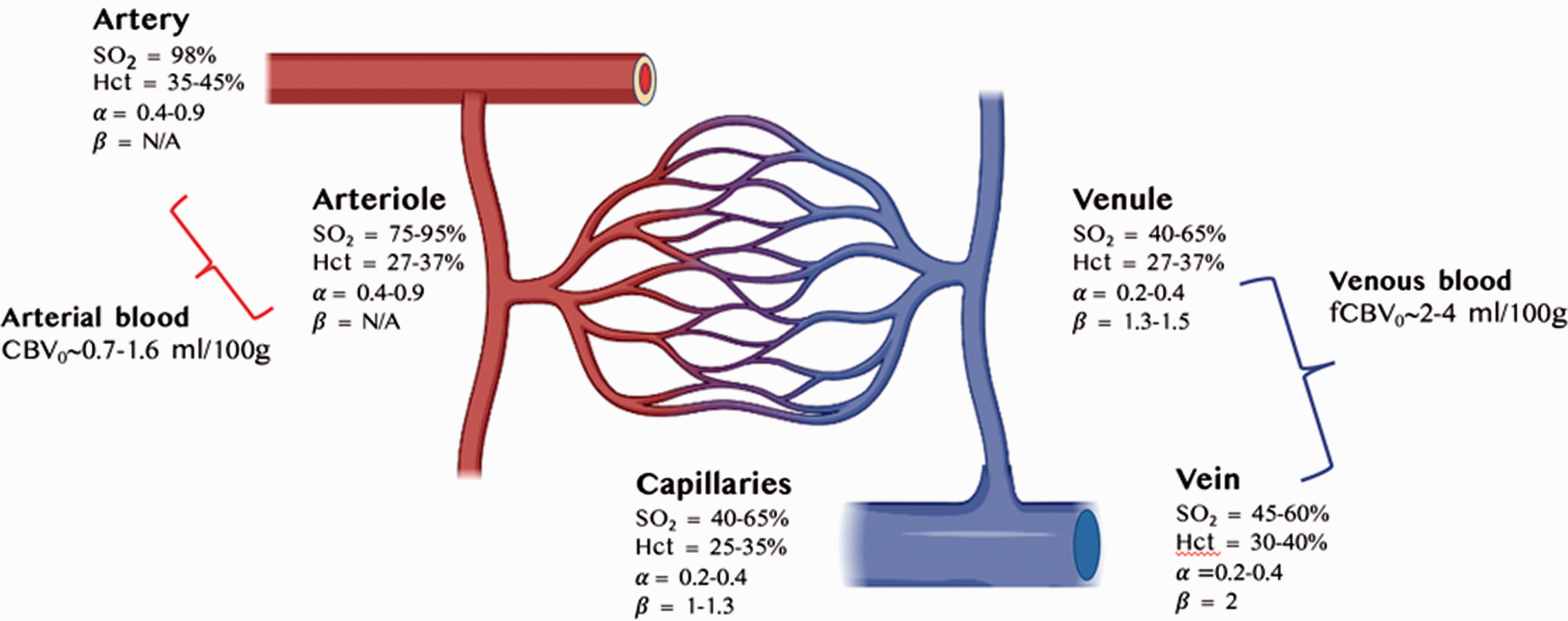
R₂′ impacted by cerebrovascular factors and assumptions across arteries, veins and capillaries in the human grey matter. Blood volume and α are taken from a recent review, ²¹⁴ hematocrit (Hct) values are taken from, ²²³ blood oxygenation (SO₂) values are taken from,^224,225 and β taken from^125,166 as well as from our own simulations (results not shown) assuming 3.0 T.

Orientation dependence of R2′

It is well known that the blood susceptibility effects underlying BOLD have an orientation dependence,^11,147 arising from dominant vascular orientations as well as the presence of neurites.^156,157 In fact, diffusion anisotropy along white matter fibres has been demonstrated to account for 37% in OEF estimates, despite claims of orientation insensitivity in white-matter OEF estimates. ¹⁵⁸ Conventionally, R₂′ mapping for calibrated BOLD addresses only the grey matter, whereby the limited spatial resolution of conventional fMRI has allowed us to neglect this fibre orientation dependence. However, with increasing spatial resolution and the popularization of laminar imaging, R₂′ orientation dependence may cease to be negligible. Recent work by Viessmann et al. ¹⁵⁹ demonstrates that the BOLD signal amplitude can vary up to 60% due to orientation differences. This trade-off between higher spatial resolution for calibrated fMRI and inclusion of effects from diffusion anisotropy along white matter fibres will be matter for future research.

Vascular size dependence of R2′

As mentioned earlier, one of the factors contributing to multiexponential R₂ (and hence R₂′) in the grey matter is the presence of diffusion across different microenvironments (i.e. blood vessels, iron, etc), which cannot be refocused by the typical spin-echo pulse. The effect of diffusion depends on the size of vessels around which the diffusion occurs. The influence of vessel size on the GESSE-based R₂′ estimate was demonstrated by Dickson et al. ¹⁶⁰ Berman et al. recently showed that ASE underestimates M due precisely to this effect. ¹⁶¹ Thus, the sampling of the SE at multiple TEs is proposed, ¹⁶¹ and accounting for the TE-dependence of R₂′ due to vascular size/diffusion effects lead to reduced M underestimation.

Vascular size, orientation and β

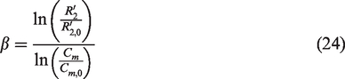
In 1993, Ogawa et al modeled the dependencies of R₂* in the presence of diffusion roughly to show that large vessels affect R₂* linearly, while small vessels affect R₂* quadratically. ¹¹ This dependence of R₂* on the susceptibility (Δχ) produced by blood within vessels was termed “β” by Davis et al. ³⁸ In essence, ΔR₂*∝ Δχ^β, where β can be determined empirically by examining the relationship between R₂′ and susceptibility levels of blood. In the work by Shu et al. ¹²⁵ β was measured in vivo across multiple regions in the white and grey matter of the rat brain by capitalizing on intravascular susceptibility variations. R₂′ was measured at different concentrations of SPIO nanoparticles contrast agent.

$$\beta =\frac{\ln \left(\frac{R_2^{\mathrm{\prime }}}{R_{2\text{,}0}^{\mathrm{\prime }}}\right)}{\ln \left(\frac{C_m^{}}{C_{m,0}^{}}\right)}$$

(24)

where C_m and C_m,0 are concentrations of contrast agent at two levels to modulate R₂′. At 9.4 T, β was found to be ∼0.8 across multiple cortical regions in the rat brain and moreover it was shown to be stable across different metabolic states.

In humans, however, the value of β is more difficult to determine empirically. Not only does β vary with vascular size, β is maximal if the blood vessels’ axes are perpendicular to B₀. But if the blood vessels are positioned parallel to the magnetic field, β is equal to zero. ¹¹⁶ In a blood vessel network, geometry of individual vessels is of less concern, but diffusion and vessel size effects still dominate, and the fact that β > 1 is due to extravascular diffusion. At one extreme, diffusion is very fast and β is 2. In the slow and intermediate diffusion regimes, however, β is between 1 and 2, depending on the choice of SE or GE sequence for measuring R_2. ¹⁶² Thus, in large vessels, such as arterioles and venules, where diffusion is viewed as slow relative to the size of the vessels, diffusion effects are outweighed by static dephasing effects and do not play any remarkable role in the BOLD contrast. For this reason also, most high field (e.g., ≥7.0 T) animal studies have usually assumed a β value of 1, ⁴¹ as signal from large veins is suppressed by the short intravascular T₂*. β may in fact drop below 1 at higher fields. However it is in the smaller capillaries, and at low fields (at 2.0 T and lower), where field inhomogeneities are much reduced, that diffusion effect on relaxation rates become significant. ¹¹⁶ For these conditions, β of 2 has been reported, as diffusion effects prevail.^11,116,163

Practically, β is often assumed based on Monte Carlo simulations at 2.0 T^146,162 which have produced a value of 1.5 for gradient-echo BOLD at 1.5 T. To date, this β value is assumed in most human calibrated fMRI studies. However, concerns have been raised regarding potential biases introduced into CMR_O2 calculation due to the assumed β.^164,165 Moreover, the interpretation of β extends beyond the dHb, embodying effects of diffusion, vascular size, CBV, tissue orientation and hematocrit among other factors (Figure 6). Very recently, a mouse cortical vascular model was inserted into the Monte Carlo framework for estimating β ¹⁶⁶ through simulations. It was found that the β value decreases with B₀. At lower field strengths, β depends on the details of the vasculature and can vary across subjects and regions for a uniform distribution of Δχ.

At high field, ΔR₂ is generally very small when compared to ΔR₂*. Additionally, ΔR₂ is uniform throughout the brain, whereas ΔR₂* (owing to ΔR₂′) is higher in superficial layers of the cortex, due to their proximity to larger veins and CSF. Previous imaging studies showed that cortical microvessels are thinner in deeper layers,^167,168 but despite the gradients observed in cortical ΔR₂′ due to vessel size or blood volume fraction differences, β values among all neocortical regions appeared homogeneous, in contrast to the implications from former simulations and analyses.^11,116,146 The smoothness of β values in the cortex suggests relatively homogeneous coupling between metabolism and hemodynamics. ¹²⁵ However, further studies with vascular staining are needed to confirm β’s physiological dependence on vessel size across regions.

Assumptions of arterial CBV

It is commonly assumed in the calibrated fMRI literature that arterial blood does not contribute to the BOLD effect. This assumption is a concern for both gas-based and gas-free calibrated fMRI. As was mentioned earlier, since oxy-Hb is diamagnetic, the iso-susceptibility oxygenation of arterial blood can be as low as 89%. ¹⁴⁷ Thus, as arterial blood is generally known to be more oxygenated than this, the susceptibility difference between arterial blood and brain parenchyma also leads to intravoxel signal dephasing and BOLD signal loss. However, the definition of “arterial” can influence the accuracy of this assumption. Early measurements in rodents have uncovered substantial precapillary O₂ loss,^169,170 which, coupled with the high elasticity of arterioles, could fundamentally alter the interpretation of BOLD signal localization. Previous studies in animals have recorded arterial O₂ decreases in the range of 10-40% with increasing degrees of branching. ¹⁷¹ If we assume the average arterial O₂ saturation is only 70% rather than 100%, the arterial-venous difference in blood oxygenation that the OEF model is based on becomes more complicated to solve for calibrated fMRI. Furthermore, the high arterial flow can introduce potential T₁-based signal perturbations to the steady state BOLD signal (i.e., inflow effects). While this is deemed a negligible effect for typical fMRI acquisition protocols, ¹⁷² the increasing adoption of shorter repetition times, such as permitted by slice-acceleration schemes.^173,174 This effect is expected to be magnified at higher field strengths. The implications of arterial-CBV participation include: (1) higher CBF-CBV coupling (exponent α in Table 1); (2) reduced BOLD signal change due to tasks; (3) the occurrence of negative BOLD response to an increase in neural activity. The latter could occur due to the small volume fraction of arterial vessels and their high capacity for expansion during activation, leading to increased intra-voxel mesoscopic B₀ inhomogeneity.

The extravascular assumption

The empirically derived calibrated fMRI model^38,101 assumes that the intravascular BOLD signal contribution is negligible, as the susceptibility effects that underlie the β parameter are dominated by extravascular mesoscopic B₀ inhomogeneities. Moreover, only blood vessels oriented perpendicular to the main magnetic field B₀ contribute to these B₀ inhomogeneities. Furthermore, this extravascular contribution depends on voxel size; in larger vessels, it is more likely that the B₀-offset effects form a complete set of dipoles that cancel each other, a scenario less likely to happen in smaller voxels. The intravascular BOLD contribution, on the other hand, has been found to range from 60%-70% at 1.5 T to 20% at 7.0 T. ¹⁷⁵ Moreover, the intravascular BOLD contribution varies with TE, being maximized when TE equals blood T₂*, with shorter TEs introducing more intravascular weighting.^176,177 It is unclear if intravascular BOLD follows the same empirical BOLD model, therefore there is a potentially sizeable portion of the BOLD signal that cannot be explained by the existing calibration process.

Assumptions specific to gas-calibrated fMRI

For children, the elderly and clinical populations, gas calibration, especially via hypercapnia, remains challenging. Safety concerns during acute hypercapnia would most likely contraindicate participants with respiratory diseases (such as asthma), pulmonary occlusions and kidney disease. Compliance and attrition issues would also in general be more likely in the above populations. ¹⁷⁸ Furthermore, there are gas-calibration specific assumptions about respiratory physiology.

Hypercapnia-related assumptions

Notwithstanding the nervous response initiation by the macrovascular CO₂ receptors, the homeostatic blood pH is actively regulated. Thus, hypercapnic challenges, in which the increased arterial CO₂ content induces large CBF increases without a significant concomitant increase in CMR_O2,^114,179 have been widely used to study cerebrovascular coupling. While the broad validity of this assumption has recently been confirmed, ¹³⁸ it is important to realize that such an assumption is only likely to hold at mild levels of hypercapnia. ¹⁷⁹ Sustained increases in arterial CO₂ is known to suppress neuronal activity,^180–182 as measured using electroencephalography ¹⁸³ and magnetoencephalography.^180,181

As typical calibrated fMRI studies are not equipped to enforce strict control on CO₂ levels, it is more feasible to account for the effect of CMR_O2. Driver et al. proposed a graded-hypercapnia under the assumption that increased CO₂ will have a concordant increase in CMR_O2. This can be used to calculate M without any knowledge of baseline CMR_O2. ¹⁰⁴

$$\frac{{\mathit{CMR}}_{O_2,HC}}{{\mathit{CMR}}_{O_2,0}}=1+\kappa \cdot \mathrm{\Delta }\mathit{PetC}{O}_2$$

(25)

where κ relates end-tidal partial pressure of CO₂ (PetCO₂) during hypercapnia (HC) to CMR_O2. This method produced M values that were on average lower, potentially as it accounts for CMR_O2 decreases incurred during hypercapnia, thus reducing the baseline-CMR_O2 underestimation. An alternative is to adopt a CO₂-free calibration method, such as hyperoxic calibration, or gas-free calibration.

Hyperoxia-related assumptions

The iso-hemodynamic assumption refers to the assumption that CBF remains unaltered during hyperoxic calibration. However, in practice, CBF has been known to decrease at high inhaled O₂ levels. ⁹³ Thus, the use of a CBF correction factor with equation (10) (Table 2) is advisable,^93,184

$$M=\frac{\frac{\Delta \mathit{BOLD}}{{\mathit{BOLD}}_0}}{1-{\mathit{CBF}}^{\alpha }·(\frac{\Delta \left[\mathit{dHb}\right]}{[Hb{]}_0}+\frac{r}{\mathit{CBF}}{)}^{\beta }}$$

(26)

where r is the correction factor for O₂-induced CBF reduction. Moreover, the generalized calibration model makes no assumptions about CBF. ⁹⁸ Beyond CBF, dissolved O₂ in the plasma has also been raised as a potential source of BOLD signal bias, as the extra O₂ delivered in hyperoxia is carried by the plasma. However, this was demonstrated not to be a notable factor.^{118,185–187}

The Hct and baseline OEF are assumed as constants in the oxygen saturation equation, but potential variations in Hct and their consequences are described in subsections to follow.

The end-tidal assumptions

Arterial partial pressure of CO₂ (PaCO₂) and O₂ (PaO₂) are in turn inferred from the PetO₂, taking into account the alveolar-arterial gas gradient and assuming that arterial blood is well equilibrated with gases in the alveoli. ⁹⁴ This latter assumption relies upon healthy lung function for validity; for instance, it would not hold in patients with pneumonia have a physical barrier within the alveoli that limits the diffusion of oxygen into the capillaries. ¹⁸⁸ In addition, the alveolar gas equation is valid only in the setting of steady-state conditions.

The assumption of the end-tidal gas levels reflecting intravascular gas levels is less critical for hypercapnic than for hyperoxic calibration. Hypercapnic calibration relies on a known relationship between PaCO₂ and CBF. Conversely, in hyperoxic calibration, [dHb]/[dHb]₀ is estimated by modeling oxygen carrying capacity of the blood as a function of the PaO₂.

Assumptions of hematocrit

The hematocrit refers to the proportion, by volume, of the blood that consists of red blood cells. The role of the hematocrit in shaping the range of hemodynamic and metabolic estimates in fMRI has become increasingly investigated.^{103,189–191} In hyperoxic, dual calibration and gas-free calibration, it is necessary to assume a baseline [Hb], which is proportional to Hct. Specifically, blood R₂ dependence on both SO₂ and Hct.^192–198 Moreover, accounting for the role of hematocrit in between-subject variations in MRI-derived baseline cerebral hemodynamic parameters. ¹⁹⁰ In a rat model, laser doppler flowmetry combined with MRI (contrast-enhanced using a plasma-borne contrast agent like SPIO nanoparticles) has been used to estimate Hct in vivo. ¹⁸⁹ In humans, the dependence of blood T₁ on Hct^199,200 has been capitalized, resulting in rapid intravascular (arterial and venous) T₁ assessment using a flow-compensated Look-Locker technique. Contrast-enhanced methods have also been proposed. ²⁰¹ Hematocrit abnormalities are observed in a number of clinical conditions. For instance, sickle cell anaemia is associated with reduced Hct, and calibrated fMRI would require blood sampling. ²⁰²

Assumptions of α

Despite the widespread use of Grubb’s relationship, ²⁰³ its adoption by Grubb et al. was based on empirical rather than theoretical discovery. Since the BOLD signal is dependent primarily upon deoxygenated, instead of total, blood volume change, the relevant ΔCBV in the context of BOLD modeling may be overestimated when using Grubb’s coefficient of 0.38, leading to the potential underestimation of ΔCMR_O2 for a given ΔCBF and ΔBOLD. Simulations show that an overestimation of α leads to an underestimation of ΔCMR_O2 with a mirroring overestimation in the neurovascular coupling ratio n.^94,204

The current consensus is that the power-law α coefficient is much lower when it concerns the BOLD-specific CBV changes, ²⁰⁴ capillary volume, ²⁰⁵ and total CBV. ²⁰³ Moreover, different parts of the brain are associated with different α values,^206–208 as are different cortical layers. ²⁰⁹ To further complicate the issue, veins and capillaries may be associated with different CBF-CBV coupling,^205,210,211 fuelling the continued debate into the differential participation of capillaries and veins in hyperemia.^{205,210,212,213} MRI-based CBV mapping methods is the topic of a recent review, ²¹⁴ and will not be reiterated here. Finally, in terms of the potential for dynamic calibration, ¹⁴⁵ the CBV-CBF relationship is far from being clear through the phase of the functional hyperemic response. ²¹⁵ In pathological conditions, α may not be accurately represented by the published values, which pertain mostly to healthy young adults. It should also be mentioned that the vasoactive mechanisms of functional and CO₂-related hyperemia are not identical. While microvascular dilation is mainly linked to the presence of Ca²⁺, the CO₂ response is believed to be mainly explained by the effect of bicarbonate ions and pH. ²¹⁶ While nitric oxide (NO) has been suggested as a mediator of CO₂-related vasodilation, the source of the NO release, whether it is the neurons or the endothelium, is still debated. This is even more relevant in pathological conditions in which either the neurons or the endothelium could be impaired, then the equivalence of the functional and vascular response may break down.

Pathologies such as small-vessel disease (SVD) have been linked to systemic inflammation, and have been associated with microbleeds as well as increased stroke risk. SVD may trigger perivascular space dysfunction leading to white-matter hyperintensities. ²¹⁷ It has been hypothesized that enlarged periventricular spaces involve inflammation and increased CMR_O2.^218,219 It has also been suggested, based on animal studies, that reduced cerebrovascular reactivity may precede the development of visible white-matter hyperintensities. ²²⁰ Moreover, SVD may be related to hypoperfusion despite the hypermetabolism, suggesting an altered neurovascular (vs. neurometabolic) coupling as well as a potential alteration in the α coefficient in SVD patients and those exhibiting perivascular enlargement.

Stroke, on the other hand, can lead to extreme alterations in the basal vascular physiology, creating a scenario in which calibrated fMRI can be particularly useful for identifying salvageable tissue. However, the type of stroke, whether haemorrhagic or ischemic, also determines the applicability of gas calibration. Moreover, one might observe a gas-calibration BOLD response while the neuronal hyperemic response is diminished or absent, violating the assumption surrounding the gas-based M value estimation. ²²¹

Summary and future outlook

Calibrated fMRI studies in animals show that neural (LFP, MUA) and hyperemic (BOLD, CBV, CBF) components are well coupled for steady-state and dynamic stimuli, lending confidence to application of the same biophysical models of calibrated fMRI for a wide range of stimulus conditions. Importantly, the CMR_O2 increases during stimuli of different epochs indicate relevance of oxidative metabolism for supporting neural events separated by less than 200 ms. While gas-free mapping of M-values used for these CMR_O2 calculations are an enticing advantage for clinical translation of calibrated fMRI, some considerations must be met as to how R₂′ values are mapped across cortical grey matter, and these same caveats may apply to the translation of calibrated fMRI to clinical populations. Given the rapid rise of calibrated fMRI studies in recent years it is expected that clinical translation with gas-free setups will be important for understanding the variations of flow-metabolism coupling in neurological and neurodegenerative patients, and for realizing the potential of calibrated fMRI.

Supplemental Material

sj-pdf-1-jcb-10.1177_0271678X221077338 - Supplemental material for Mapping oxidative metabolism in the human brain with calibrated fMRI in health and disease

Supplemental material, sj-pdf-1-jcb-10.1177_0271678X221077338 for Mapping oxidative metabolism in the human brain with calibrated fMRI in health and disease by J Jean Chen, Biranavan Uthayakumar and Fahmeed Hyder in Journal of Cerebral Blood Flow & Metabolism