Sage Journals: Discover world-class research

Abstract

Elevated carbon dioxide (CO2) in breathing air is widely used as a vasoactive stimulus to assess cerebrovascular functions under hypercapnia (i.e., “stress test” for the brain). Blood-oxygen-level-dependent (BOLD) is a contrast mechanism used in functional magnetic resonance imaging (fMRI). BOLD is used to study CO2-induced cerebrovascular reactivity (CVR), which is defined as the voxel-wise percentage BOLD signal change per mmHg change in the arterial partial pressure of CO2 (PaCO2). Besides the CVR, two additional important parameters reflecting the cerebrovascular functions are the arrival time of arterial CO2 at each voxel, and the waveform of the local BOLD signal. In this study, we developed a novel analytical method to accurately calculate the arrival time of elevated CO2 at each voxel using the systemic low frequency oscillations (sLFO: 0.01-0.1 Hz) extracted from the CO2 challenge data. In addition, 26 candidate hemodynamic response functions (HRF) were used to quantitatively describe the temporal brain reactions to a CO2 stimulus. We demonstrated that our approach improved the traditional method by allowing us to accurately map three perfusion-related parameters: the relative arrival time of blood, the hemodynamic response function, and CVR during a CO2 challenge.

Keywords

Low frequency oscillation cerebrovascular reactivity hemodynamic response hypercapnia BOLD signal

Introduction

CO2 is a potent vessel dilator. An increase in arterial CO2 will lead to smooth muscle cell relaxation in the arteries, and consequently vasodilatation. Cerebral blood flow (CBF) will then increase as a result.¹ A CO2 challenge is an ideal vasodilation stimulus in terms of practicality and standardization.² Therefore, a CO2 challenge can be used as a “stress test” for the brain to expose defects in the tight coupling between magnitude of applied CO2 and CBF resulting from brain injury and disease states, such as Moyamoya,³ stroke,⁴ arterial stenosis,⁵ and traumatic brain injury.^6,7

A widely used parameter to measure the brain’s reaction to a CO2 challenge is cerebrovascular reactivity (CVR), defined as the percentage signal change in CBF per mmHg change in arterial partial pressure of CO2 (PaCO2).⁵ In practice, the end-tidal partial pressure of CO2 (P_ETCO2) is considered as a non-invasive approximation of the PaCO2.^8,9 An increase in CBF lowers the deoxy-hemoglobin concentration, leading to an increase in blood oxygenation level-dependent (BOLD) functional MRI (fMRI) signal. In addition, compared to other MRI acquisition techniques (e.g., arterial spin labeling (ASL)), BOLD fMRI has superior sensitivity and temporal resolution. Therefore, BOLD signals have generally been used as a surrogate marker for measuring changes in regional CBF, and BOLD fMRI is the most widely used MRI technique for CVR mapping.^2,5,10 However, BOLD fMRI signals are complicated, which reflect a dynamic interplay among CBF, CBV, and cerebral metabolic rate of oxygen. A non-linear relationship has also been reported recently between BOLD and blood CO2 content.¹¹ The CO2-induced regional distribution of blood flow is also complicated, which depends on the local vasculature and the magnitude of applied vasoactive stimulus due to the existence of the P_ETCO2-dependent-flow-responses between gray matter (GM) and white matter (WM), and even between different layers of WM (outer->inner->deep).^12,13

CVR experiments can simultaneously measure the BOLD signal and the P_ETCO2. However, this method is commonly over-simplified under the assumptions that the elevated CO2 arrives at all voxels at the same time, and it causes the same temporal change in any fMRI signal. These assumptions might affect the accuracy of a CVR measurement.

A CO2 challenge initiates a complicated process in the brain, comprised of two critical steps: transport and reaction. Transport: The elevated CO2 in the lungs diffuses across the alveoli into the blood. It is then transported by the blood to the brain. As a result of the cerebrovasculature, the diffused CO2 will arrive at different locations within the brain at varying times. Reaction: Upon arrival, the elevated CO2 triggers reactions in the local tissue and vessels. These reactions to CO2 can be categorized by the dynamics and the magnitude of the vascular response. The former refers to the form of the local BOLD temporal waveform, a consequence of the interaction between the local hemodynamic response and the incoming CO2 waveform. The latter is typically represented by local CVR values. Some recent studies have focused on the spatial-specific BOLD waveform/hemodynamic response functions (HRFs) during a CO2 challenge.^3,5,10,14 Other studies have focused on determining the arrival time of the CO2.^3,15–17 Duffin et al.³ obtained a phase map to describe the response time using transfer function analysis. Poublanc et al.⁵ utilized the time constant of a linear first-order exponential curve to represent the different response time to the CO2 stimulus. More recently, Prokopiou et al.¹⁰ utilized a kernel based on Laguerre and gamma functions to estimate voxel-specific HRFs in selected ROIs, suggesting that there may be different HRF characteristics across different locations. However, no studies to date have taken the different CO2 arrival times into the consideration when estimating HRFs, which could affect their accuracy. It is known that the HRF in the CO2 challenge data reflects the reaction of the blood vessel to the elevated CO2, which may include its own delays. It is crucial to separate the delay times of the blood transport (i.e., times for the CO2 to travel to different regions) from those of the vessel responses (i.e., occurring after the arrival of CO2). Thus, knowing the exact arrival time of the elevated CO2 will benefit the derivation of accurate HRFs and subsequently, the CVR values.

In this study, we exploited the systemic low frequency oscillations (sLFO: 0.01∼0.1 Hz) in BOLD signal to calculate the arrival time of elevated CO2. sLFOs have been widely observed in BOLD signals in resting state (RS) fMRI data with time delays. The delay is found to be closely related to the blood arrival time (BAT) for the corresponding voxel, as supported by gadolinium-based dynamic susceptibility contrast MR.¹⁸ The method has not yet been used to track the arrival of the elevated CO2 in hypercapnia data. The main purpose of this study was to accurately calculate the relative arrival time (rAT) of the elevated CO2 using sLFOs, and use these rAT maps to derive more accurate HRFs and CVR maps across different brain regions.

Materials and methods

Data acquisition

CO2 challenges were performed on 11 healthy volunteers (F:5; M:6, age ± SD: 22.7 ± 4.4 years; 3 subjects were subsequently excluded due to dropouts and/or poor data quality). This study was approved by the Purdue University Institutional Review Board (IRB Study 1706019332) and all participants had given written informed consent. The entire study complies with federal regulations at 45 CFR 46 and 21 CFR 50 and 56.

FMRI data were obtained from a 3 T GE Discovery MR750 MR scanner at the university’s Engineering MRI Facility. All data were acquired using a 32-channel NOVA Medical receive coil. The MRI scans began with a T1-weighted structural scan (TR/TE = 4800/1000 ms, voxel size = 1 × 0.97 × 0.97 mm³, FOV =250 × 250 mm², slice thickness = 1 mm, scan length =2 min 6 sec and slices per slab = 168), followed by two echo planar imaging (EPI) scans (FOV = 216 ×216 mm², acquisition matrix = 72 × 72, 60 slices, slice thickness = 3 mm, voxel size = 3 × 3 × 3 mm³, TR/TE = 1000/30 ms, flip angle = 50°, hyperband acceleration factor = 4, phase acceleration factor = 1, scan-length = 10 min).The first scan assessed RS functional connectivity, while the second scan was used for hypercapnia assessment.

In the hypercapnia scan, the CO2 challenge was given via a programmable computer-based gas delivery system: RespirAct™ (Thornhill Research Inc. Toronto, Canada).¹⁹ A plastic face mask connected with a breathing circuit was taped on each subject’s face prior to entering the MRI scanner room (a valve permitted subjects to breathe the room air when the partial pressure of CO2 was not being regulated—e.g., during the RS scan). The breathing protocol was set as: two 2-minute blocks of CO2 of 10 mmHg higher than baseline with 2-minute baseline before, in between and after the CO2 stimulus (see Figure 1). The P_ETCO2 was measured and controlled by the RespirAct™. A comparison of gas delivery systems can be found in the previous publication.⁸ The initiations of the gas challenge and the MRI recording were synchronized by two independent operators.

Figure 1.

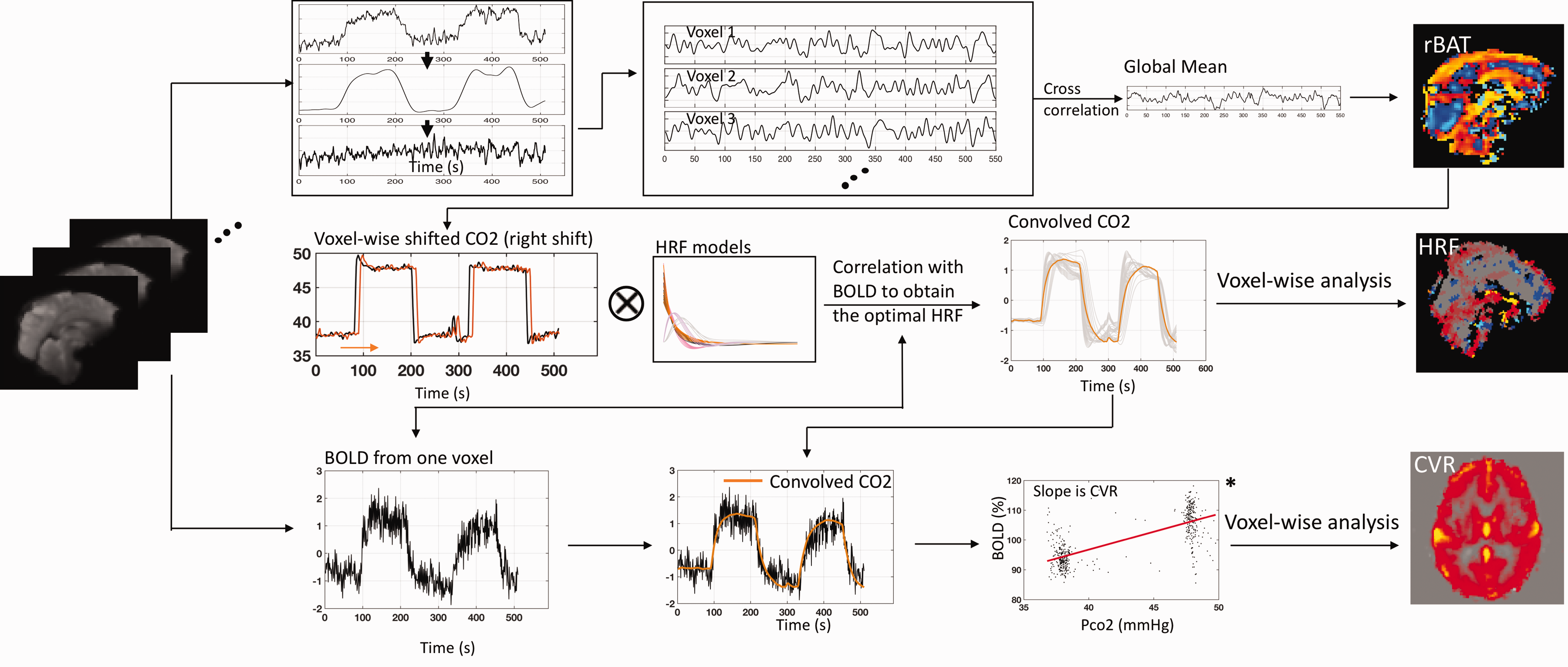
Methodology for quantitatively characterizing the brain’s reactions to the CO2 challenge. A relative arrival map (rAT) was obtained using systemic low frequency oscillation from BOLD (Top panel). After shifting the P_ETCO2 waveform (obtained from RespirAct™) based on the rAT map and convolving it with a set of candidate hemodynamic response functions (HRFs: see Figure 2), the voxel-wise optimal HRF was identified by the maximal correlation between observed BOLD signal and the convolved P_ETCO2 waveform (Middle panel). An improved cerebrovascular reactivity (CVR) map was then obtained by performing a linear fit between the BOLD percentage change and the convolved P_ETCO2 change (in mmHg), with the slope of this fit line being the CVR value (unit: %/mmHg) (see *; Bottom panel).

Data processing

Acquired data were processed using the FMRIB Software Library (FSL, FMRIB Expert Analysis Tool, v6.01, http://www.fmrib.ox.ac.uk/fsl, Oxford University, UK),²⁰ and locally developed programs in MATLAB (version 2017a; The MathWorks Inc., Natick, MA). The fMRI data were preprocessed as recommended by Power et al., including motion correction (FSL mcflirt) and spatial smoothing with a three-dimensional isotropic Gaussian kernel (full‐width half‐maximum = 5 mm).²¹

Relative arrival time (rAT) map

For each subject, first, the very low frequency oscillations (vLFO: 0.001∼0.02 Hz) were removed from the BOLD signals in both RS and CO2 challenge data (see details below). Secondly, a zero-delay bandpass filter (0.01–0.1 Hz, 4th order) was used to extract the sLFO from the BOLD of global mean and each voxel. Thirdly, a voxel-wise cross-correlation was conducted between the sLFO from global mean and each voxel. The delay time corresponding to the maximum cross-correlation coefficient (MCCC) is believed to represent the rAT for the corresponding voxel.²² To obtain the delay values of high temporal resolution (sub-second), all the time series were oversampled from 1 s (i.e., TR) to 0.1 s. A paired-t test was performed to compare the RS and the hypercapnia rAT maps. Note, due to the facts that the propagation of sLFO is not fully understood and it is an indirect measurement of perfusion, the resulting map is named as the arrival time map (AT, the arrival of the sLFO), instead of the BAT map.

Since the BOLD signal has been heavily modulated at a vLFO (1/240 Hz) by the CO2 challenge (i.e. P_ETCO2-related-vLFO), an additional step was performed to demodulate and recover the sLFO (i.e., sLFO (CO2-demodulated)) in each voxel (see Figure 1). In detail, we extracted the P_ETCO2-related-vLFO signal (0.001-0.02 Hz) using a bandpass filter and regress it from the original BOLD signal by subtraction. The implemented method is focused on removal of the effects of the primary modulation frequency (1/240 Hz) and its 1st harmonic. To be consistent with the procedures from hypercapnia data, we applied the same steps in RS data.

Alignment of P_ETCO2 measurement

Since the rAT only represents the relative delay time with reference to a global mean, the absolute CO2 arrival time for each individual voxel needs to be computed by adding an offset related to the P_ETCO2 measurement (obtained from RespirAct™) to the voxel-specific rAT value. Specifically, we define the absolute CO2 arrival time ( $T_{abs}$ ) as the sum of the P_ETCO₂-to-reference delay and the reference-to-voxel delay, described hereafter.

To calculate the P_ETCO₂-to-reference delay, reference voxels were selected by cross-correlating each voxel’s unfiltered BOLD and the corresponding P_ETCO2 measurement. A set of “reference voxels” was defined by brain voxels having the shortest extra-cerebral delays—i.e., those in the range of 1–3.5% of the entire brain, noting that the top 1% were excluded as they typically correspond to unrealistically short delays arising from spurious correlation error. The average delay over these reference voxels was taken as the P_ETCO₂-to-reference delay ( $T_{P_{E T} C O_{2} t o ref}$ ), an absolute time measure accounting for the “lung-to-brain” time^8,23,24 (the travel time between the mouthpiece to the analyzer has been calibrated). Note that most of the reference voxels reside in artery-rich regions (i.e., internal carotid arteries) given that these are the first vessels/regions where the blood enters the brain. The BOLD effects in those regions are relatively weak due to the lack of deoxyhemoglobin. The non-BOLD contrast is from partial volume effects or the flow effects.^22,25,26 Given that the P_ETCO2-related-vLFOs are much stronger in CO2 challenge due to the vasodilation and increase in blood flow (non-BOLD contrast) than the sLFOs (CO2-demodulated), we used the P_ETCO2-related-vLFOs to identify the voxels of early AT, instead of using sLFO (CO2-demodulated) signals.

The voxel-specific CO2 AT was then computed in conjunction with analysis of the rAT map. First, the average rAT value over the same reference voxels (T_{rAT_ref}) was computed, providing a reference offset associated with the arrival of CO2 within the brain. The voxel-specific delay was then calculated as the difference between the rAT value for any given voxel $(T_{rAT voxel})$ and this reference. Given that both of these measures are “relative” with respect to a common quantity (the global mean), the difference ( $T_{ref t o voxel}$ ) represents an absolute delay for the given voxel relative to the reference CO2 arrival time. Finally, the absolute CO2 AT at each voxel ( $T_{abs}$ ) was computed by adding the absolute voxel delay to the overall minimum CO2 arrival delay:

T_{ref t o voxel} = T_{rAT voxel} - T_{{rAT}_{-} r e f}

(1)

T_{abs} = T_{P_{E T} C O_{2} t o ref} + T_{ref t o voxel}

(2)

$T_{abs}$ : Absolute CO2 AT at each voxel;

$T_{P_{E T} C O_{2} t o ref}$ : Extra-cerebral delay before reaching the reference voxels (using CO2 waveform);

$T_{ref t o voxel}$ : Cerebral delays from reference voxels to each voxel (using sLFOs (CO2-demodulated));

$T_{rAT voxel}$ : rAT of the given voxel;

$T_{rAT ref}$ : Averaged rAT values of the reference voxels.

Hemodynamic Response Function (HRF) map

After calculating the exact AT of the CO2 waveform at each voxel, the corresponding HRF that reflects the local reaction (waveform) can be modeled. Based on Shan et al.,²⁷ we employed the double gamma model, which exhibited the best performance in parameter accuracy and identifiability among five evaluated HRF models. To achieve physiologically-realistic solutions, a fixed number of HRFs were used to represent a wide range of reactions based on Poublanc et al.⁵ In our model, provided below, we limited the number of parameters to three that affect different aspects of the HRF (see Figure 2)— $α_{1}$ : predominantly controlling the response delay (time to peak); $β_{1}$ : predominantly controlling the shape variant (maximum and slope) of the HRF; and $β_{2}$ : predominantly controlling the undershoot. We developed two sets of constrained ranges for each parameter based on the ranges used by Shan et al.²⁷: (A) $α_{1} = 1, β_{1} = (10, 12, 14, 16, 18, 20), β_{2} = 10, 20, 40$ ; (B) $α_{1} = (2, {3), β}_{1} = (14, 16, 18, 20), β_{2} = 10$ . These parameter sets resulted in 26 possible candidate HRFs. We roughly numbered the candidate HRFs according to the slope (i.e., response speed) of the first increasing stage of the convolved elevated CO2, such that a higher number HRF indicates a longer/slower response to the elevated CO2. $h (t) = \frac{t^{α_{1} - 1} {β_{1}}^{- α_{1}} e^{{- β}_{1}^{- 1} t}}{Γ (α_{1})} - \frac{t^{α_{2} - 1} {β_{2}}^{{- α}_{2}} e^{{- β}_{2}^{- 1} t}}{2 Γ (α_{2})}; α_{2} = α_{1} + 4$ $where 0 < t < 200 seconds, with increment o f 1 second$

Figure 2.

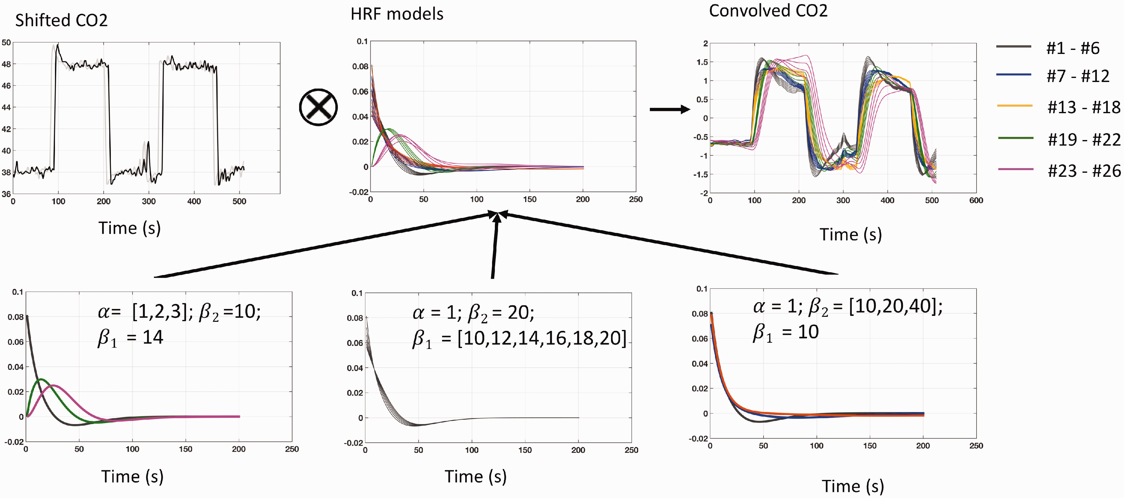
Generation of the candidate hemodynamic response function (HRF) models. (Top) In the proposed method, the shifted P_ETCO2 waveform was convolved with different HRFs to identify the best approximation of the observed BOLD signal. (Bottom) Three parameters ( $α_{1}$ , $β_{1}$ , and $β_{2}$ ) were varied in the proposed model, producing 26 candidate HRFs. The response delay (time to peak) is predominantly charged by $α$ (bottom left); The shape variant of the HRF is predominantly charged by $β_{1}$ (the maximum; bottom middle) and $β_{2}$ (the undershoot; bottom right).

Note that all candidate HRFs were normalized (divided by the area under the curve via MATLAB trapz).

To find the voxel-specific optimal HRF, the 26 candidate HRFs were convolved with the shifted P_ETCO2 waveform (based on the exact CO2 arrival time) to obtain the convolved P_ETCO2 waveforms. The HRF corresponding to the convolved P_ETCO2 waveform having the maximal correlation with the BOLD signal for a particular voxel was taken as its optimal HRF. Three characteristic metrics of the HRFs were also derived based on Lindquist et al.,²⁸ which are the height (the magnitude of the peak), the width (full width at half maximum (FWHM) in second), and the time to peak (TTP; in second).

Cerebrovascular reactivity (CVR) map

The CVR value was calculated as suggested by Poublanc et al.,⁵ being the slope of a linear regression between the percentage change of the BOLD signal and the convolved P_ETCO2 in mmHg (see the plot denoted by * in Figure 1). In this case, the corresponding R² (calculated by performing the linear regression) was taken to indicate the variance in the BOLD signal explained by the convolved P_ETCO2, reflecting the goodness of fit and the accuracy of the CVR value.^14,29 Note that, to maintain the same scale as the actual P_ETCO2, the convolved P_ETCO2 was multiplied by a factor, which was determined by minimizing the mean square error between the convolved P_ETCO2 and the actual P_ETCO2. CVR maps using the traditional approaches were also obtained for comparison. One traditional approach used shifted P_ETCO2 (based on the global mean BOLD signal). The other traditional approach used convolved P_ETCO2 (with a general HRF) after shifting.^14,29,30 The mean GM and WM CVR were calculated. Paired t-tests were performed between the CVR maps from the proposed method and two traditional methods. The voxel-specific R²-difference values between the proposed method and two traditional approaches were calculated at an individual level. Positive and negative R²-difference values were derived (positive indicates increase of R² from the proposed method) and represented by a violin plot.³¹ The means and standard deviations of these positive and negative R²-difference values were computed separately for the overall population. Since the distributions of the positive and the negative R² value changes are not normal (as the result of Shapiro-Wilk test), two-sided Mann-Whitney U-test with 5% confidence level was used to evaluate the R²-difference between those at the individual level.

Simulation to assess delay accuracy

To quantify the errors of the time delay calculation, we conducted a simulation, in which, the cross-correlations (with temporal window of ±10 s as used in the study) were calculated between a real BOLD signal of CO2 challenge and itself with added white noise at various levels (a band pass filter 0.01–0.1 Hz was applied after removing the P_ETCO2-related-vLFO). The added white noise had magnitudes ranging from 0.1–7 times that of the BOLD signal (the range was selected based on the SNR of the real fMRI data) with an increment of 0.0001. The MCCCs and the corresponding delay times were calculated for each combination (BOLD v.s. BOLD + noise). The expected delay value is 0 s. Lastly, a similar simulation was carried out for the same BOLD signal in very low frequencies. Accordingly, the low pass filter 0.1 Hz was applied to remove unrealistic high frequency white noise and the temporal window was set to be ±30 s, as used in the study. (The corresponding MATLAB code and sample data can be found in the supplemental material.)

Results

Relative arrival time (rAT) maps

rAT data derived on a single subject and group (averaged over eight subjects) basis from the RS-fMRI and the hypercapnia data are presented in Figure 3(a) and (b), respectively, with the corresponding rAT scatter plots and rAT distributions plots. Observe from Figure 3, columns (i) and (ii), that the delay maps derived from the RS-fMRI data and the CO2 challenge data are similar in spatial structure, indicating that a similar sequence of the AT measurements were derived from both conditions. This perception is supported by the scatter plots in column (iii), in which the dominant axis (red fitted line) in each plot has a slope close to unity (which would be observed for identical rAT values across the scans). The difference (between the red fitted line and unity) indicates that blood flow was faster during the CO2 challenge experiment. This observation is consistent with the distributions plots of the averaged rAT maps in column (iv), wherein the spread of averaged rAT values obtained from RS-fMRI is always “wider” than that derived from the CO2 challenge data (i.e., about 0.5 s difference at full width at half maximum). Significant reduced rAT of the precentral gyrus (see arrows in Figure 3) in the prefrontal lobe was found in the hypercapnia (p = 0.001 uncorrected); the difference map on the rAT can be found in the supplemental material Figure S3).

Figure 3.

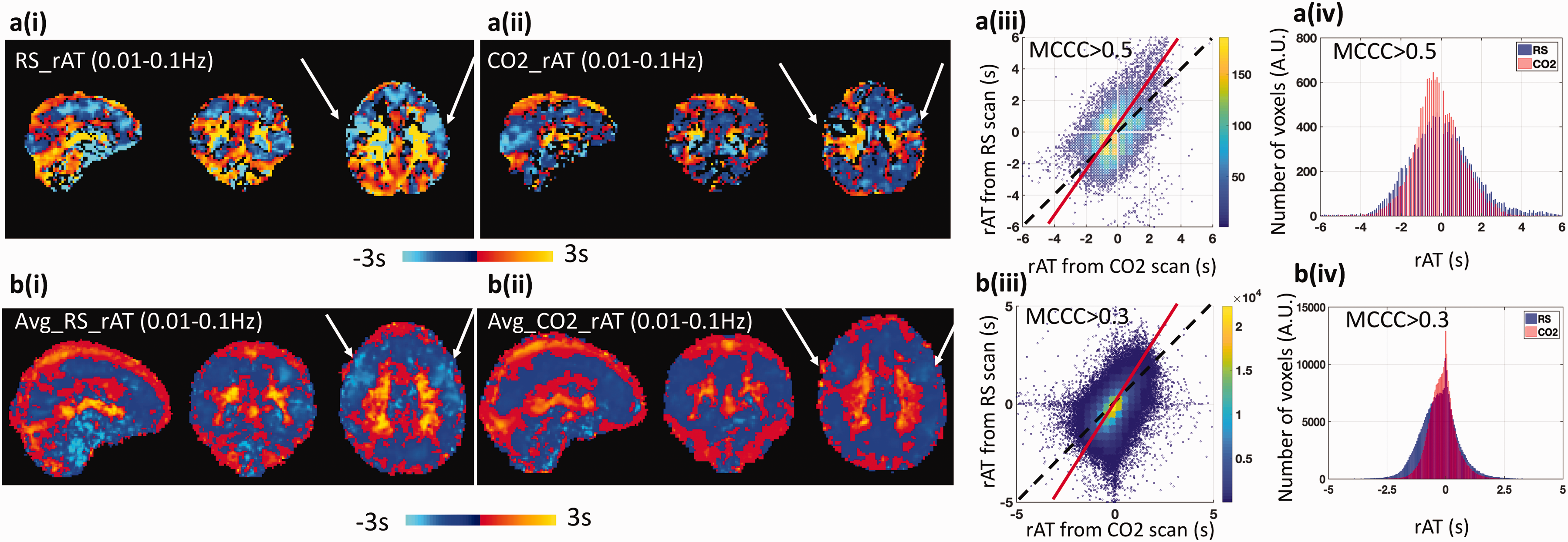
Comparison of the relative arrival time (rAT) map obtained from resting state fMRI (RS-fMRI) data and the CO2 challenge fMRI data. Top panel (a) present the results obtained from a single subject, while bottom panel (b) are the results averaged over 8 subjects. (i) rAT maps derived from RS-fMRI. (ii) rAT maps derived from the CO2 challenge data. (iii) Scatter plots comparing rAT values obtained from RS-fMRI and the CO2 challenge data. The dashed lines represent a slope of 1 (i.e., the same rAT values in each voxel obtained from RS-fMRI and the CO2 challenge data), while the solid red lines represent the fitted dominant axis of the correlation. The steeper red lines indicate that the blood generally travels faster under CO2 challenge than in RS. (iv) Comparison of the distribution of rAT values obtained from RS-fMRI and the CO2 challenge data. Note that the width (measured by the full-width at half maximum) in the CO2 challenge data is smaller than that observed for the RS-fMRI data. The threshold of the maximum cross-correlation coefficient (MCCC) for graphs a(iii) and a(iv) was 0.5, while the threshold for graphs b(iii) and b(iv) was 0.3.

Hemodynamic response function (HRF) maps

Optimized HRF maps for all subjects are shown in Figure 4(a). The color associated with each voxel represents the number (1–26) corresponding to the best-fitting HRF. The corresponding characteristic metrics of the HRFs are shown in Figure 4(b) (the height), (c) (the FWHM), and (d) (TTP). In most subjects, the HRF and the metric maps were largely symmetric between the hemispheres (based on the spatial correlation between two hemispheres using fslcc in FSL software. The results can be found in the supplemental materials Figure S4). Clear spatial-specific patterns are shown in eight subjects who were ranked based on the similarity of distributions of optimized HRFs. Note that subjects 7 and 8 had a higher number of candidate HRFs that exceeded HRF #20—i.e., slower responses to CO2. Brain tissues/structures, such as GM, WM and ventricles, can be differentiable in the HRF’s number, height, and the FWHM maps. However, the TTP maps were more homogeneous across the whole brain, due to the fact that 18 out of 26 HRFs display monoexponentially decay (with various rates). Note that black voxels were those that did not pass the thresholding in the AT maps.

Figure 4.

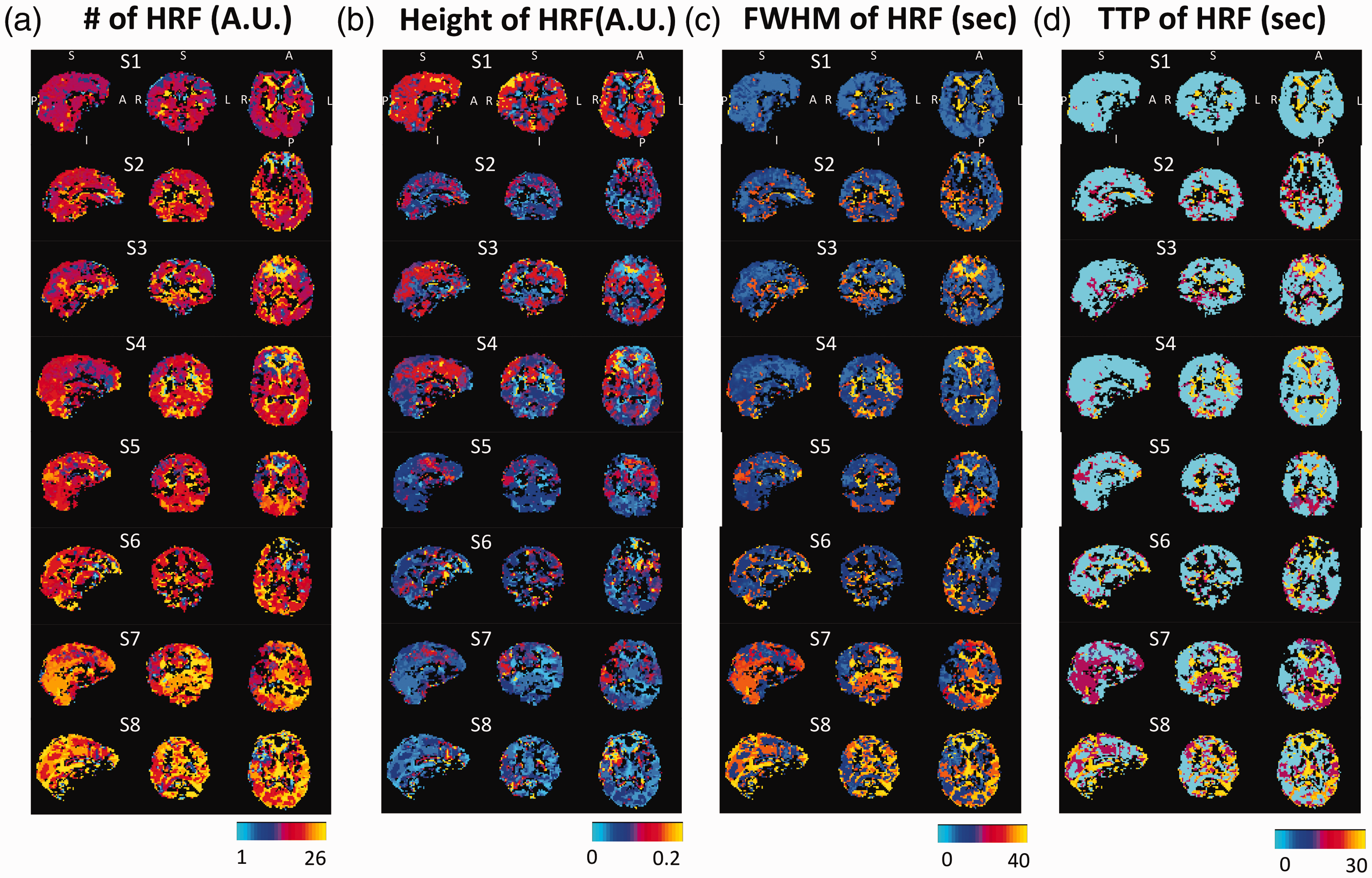
Optimized hemodynamic response function (HRF) maps (a) and the maps of characteristic metrics in height (b), FWHM (c), and TTP (d) for eight subjects. Those black voxels are those voxels do not pass the thresholding in the AT maps (MCCC < 0.3). To note that all subjects were displayed at the same coordinate with the same order.

Cerebrovascular reactivity (CVR) maps

Figure 5 presents averaged CVR maps using the two traditional methods (a-b) and the proposed method (c). The mean GM CVR and mean WM CVR values of our proposed method were 0.31 ± 0.05%ΔBOLD/mmHg and 0.16 ± 0.05%ΔBOLD/mmHg, respectively. There was no significant difference between our proposed method and two traditional methods under the false discovery rate (FDR) correction at 0.05. However, CVR differences can be found in big veins (e.g., superior sagittal sinus) and white matter (The maps of the CVR differences can be found in the supplemental material Figure S5). Negative CVR values were also observed, which were attributed to the vascular “steal effect”, the inflow effect or the partial volume effects at the brain-CSF interface.^{10,15,16,32,33}

Figure 5.

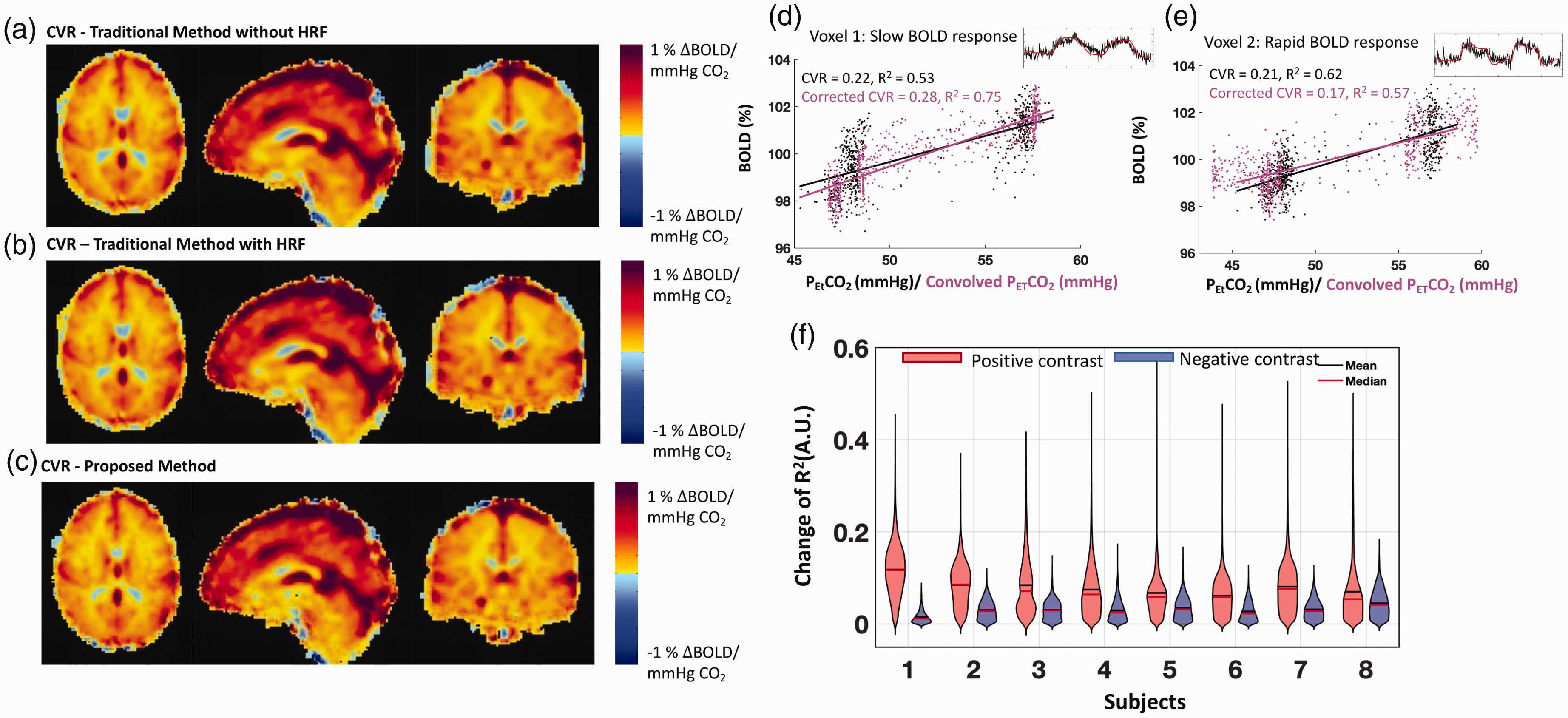
Cerebrovascular reactivity (CVR) maps obtained using the traditional methods ((a) & (b)), and the proposed method (c) are shown on the left. The mean GM CVR and mean WM CVR values of our proposed method are 0.31 ± 0.05%ΔBOLD/mmHg and 0.16 ± 0.05%ΔBOLD/mmHg, respectively. Comparison of the performance of the traditional method and the proposed method in CVR calculation is shown on the right ((d), (e) & (f)). Demonstrations of obtaining a CVR value for a voxel is shown in (d) and (e). Black dots and the corresponding fitted line represent the traditional method. Magenta dots and their corresponding linear fitted lines represent the proposed method. Original BOLD signals (with different vascular response) were shown on the right upper corner of each plot. The R²-difference values are shown in the violin plot (f), which is presented for each subject after separating positive and negative changes. On average, about 80% of the voxels for each subject show increases in R² values (mean ± S.D.: 78.9% ± 11.8%). The means and standard deviations of the eight subjects in R²-differece values are (positive) +0.08 ± 0.02 and (negative) −0.03 ± 0.008. The results of the two-sided Mann-Whitney U-test show that there is a significant difference between the positive and the negative R² value changes for each subject (P < 0.05).

Voxel-specific comparisons of the CVR calculation methodologies are highlighted in Figure 5(d) and (e) for two voxels. Note that the corresponding best-fit lines, CVR values and R² values are also presented in each plot. These two voxels exhibited two scenarios. The new method overall improved the fitting (magenta dots) with higher R² values (5d), while, sometimes, it can also produce the result with a lower R² 5(e). Note that the positive R² changes did not always result in higher CVR values (An example BOLD signal and a simulation can be found in the supplemental material Figure S6).Quantitative assessment of the changes in R² values between our proposed method and the traditional method without HRF is presented in Figure 5(f). Separating the positive (red) and negative (blue) changes in R² led to the given violin plots for each subject. On average, positive R² changes were found in 80% voxels in the brain, and 4% ± 1% voxels had the increased R² values that were greater than the two standard deviations above the mean values. Compared to the traditional method without HRF, only 56% voxels had R² value increased when using the other traditional method (with a fixed HRF) (see supplemental material Figure S5). These results indicate that the proposed method outperforms the traditional methods in fitting the BOLD signals.

Errors in the delay calculations

For the result of LFO (0.01–0.1 Hz), the scatter plot of MCCCs and corresponding delays is shown in Figure 6(a). It is obvious that higher MCCC values led to more accurate delays (closer to 0 s). The delays were less informative and distributed equally over a wide temporal range (−10 ∼10 s), when the MCCC was below 0.3. From the corresponding histogram of all the delays with MCCC > 0.3 (Figure 6(b)), 53.1% of the delays were within ±0.5 s of 0 s (i.e., the true value), and 75.4% of the delays were within ±1.0 s.

Figure 6.

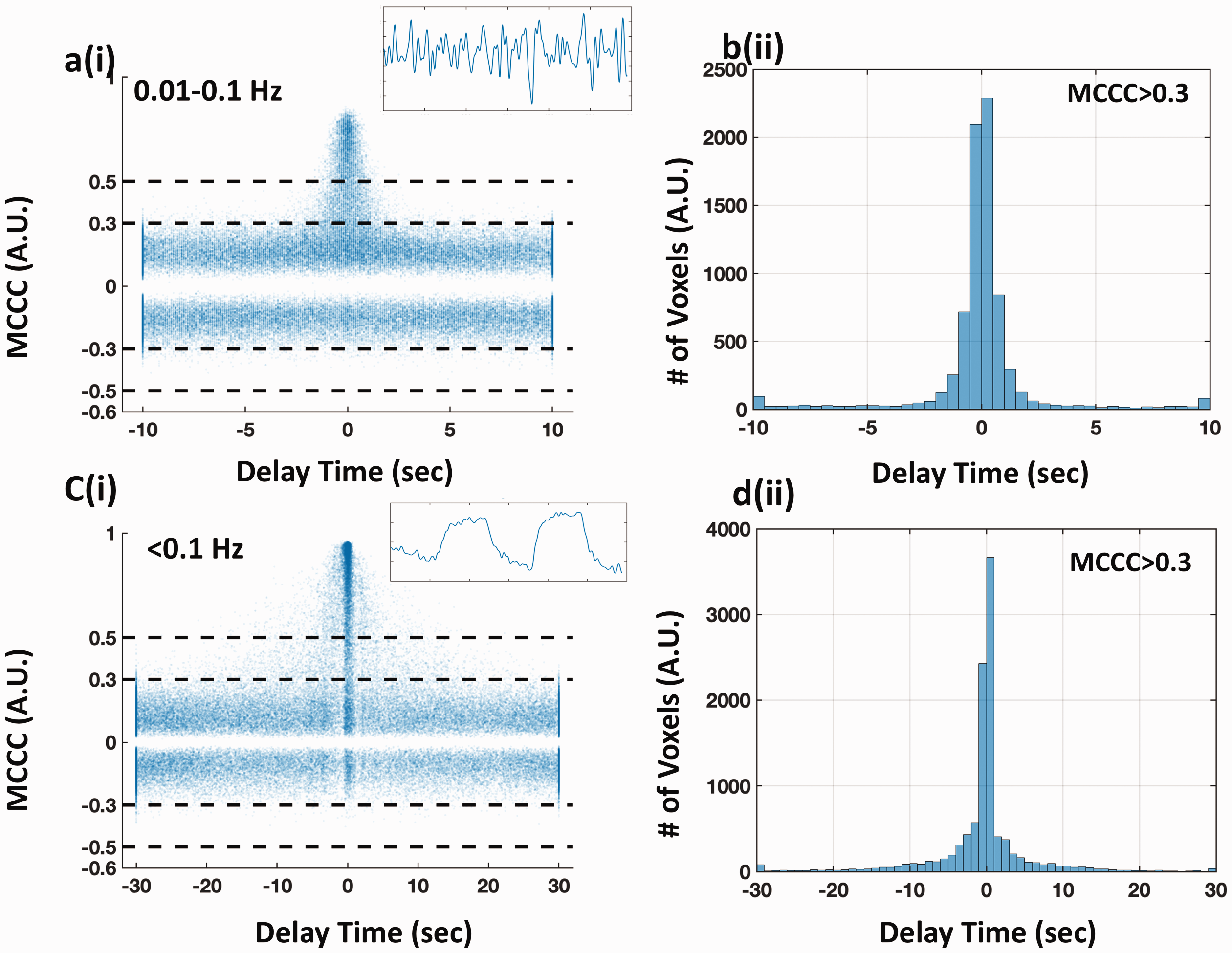
Simulation of evaluating the effect of noise on the robustness of the cross-correlation. The scatter plots of MCCCs and the corresponding delay times from cross-correlation between the original BOLD signal (with dominant frequency 0.01-0.1 Hz in (a-b) and ∼0.004 Hz in (c-d)) and itself with add-on various levels of white noise are shown in column (i). The corresponding histogram of the delay times (MCCC > 0.3) are shown in column (ii). The original BOLD signals are shown as inset figures on the upper right corners in (a) and (c).

For the result of P_ETCO2-related-vLFO, the scatter plot is shown in Figure 6(c). Compared to the result of LFO, the errors of the delay calculations increased with a broadened delay distribution. 43.2% of the delays were within ±0.5 s of the true value, and 55.5% of the delays were within ±1.0 s, when using the same threshold (MCCC > 0.3). This observation is consistent with a previous publication,³⁴ which stated that the impact of signal noise to cross-correlation accuracy is larger with lower signal frequency.

Discussions

CO2 arrival time

Many previous studies have used the sLFO in RS-fMRI data to track blood flow;^22,35–37 however, it remains unknown whether sLFOs exist in CO2 challenge fMRI data, and, if so, how they would behave. One major finding of this study is that sLFOs (CO2-demodulated) were successfully identified in CO2 challenge fMRI data. We also showed that the dynamic pattern of the sLFOs remains indicative of blood flow during the CO2 challenge, as with RS-fMRI. As previously demonstrated, the similar spatial patterns in delay maps calculated using sLFOs in both conditions indicate similar sequence of the blood arrival. Further, the time it took for the blood to travel through the brain (i.e., range of delay times) was shorter in the CO2 challenge experiment than that in the RS-fMRI, indicating that the elevated CO2 acted as a vasodilator and reduced the transit time. This is in line with a study by Ito et al.,³⁸ which demonstrated the decreased mean transit time (i.e., 0.6 s in the cerebral cortex) during hypercapnia using positron emission topography. Several ASL studies have also reported that the bolus AT to brain tissue is shortened in hypercapnia.^39–41 However, it is worth noting that the transit time (or the AT) was obtained from the CO2 challenge data with alternate periods of normocapnia and hypercapnia. Thus, the transit time was the averaged result from all the periods. We predict that the transit time could be even shorter during the period of hypercapnia. However, the duration of hypercapnia (2 min) was too short to extract reliable sLFO signals (0.01∼0.1 Hz) and conduct cross-correlation.

This new method provides insight into how sLFOs behave, from which we gain new knowledge regarding blood flow in hypercapnia. The precentral gyrus showed the largest blood velocity increase. However, a similar trend could not be observed in the areas of veins and WM. This observation is consistent with the fact that vasodilation has a strong and immediate effect on the arteries and arterioles,¹ not on veins.

Even though the physiological origin of sLFOs remains unclear, many studies have demonstrated that there exists a close link between the oscillations and vasomotion.^14,29,42,43 In this case, we demonstrate the co-existence of sLFOs (CO2-demodulated) (possibly due to vasomotion) and CO2-induced vasodilation, which implies that the dilation/constriction of the vessel wall may be modulated independently by multiple physiological processes, as long as none of the processes “saturates” the wall (i.e., dilating the vessel to its maximal size). This is an intriguing finding from which more targeted studies might help explain the origin and function of the sLFOs.

Possible errors in assessing CO2 arrival time

Arrival time of CO2 in the hypercapnia studies have been assessed by a variety of methods previously. Some of these include frequency-based methods which manipulated the stimulus waveforms to derive the voxel-specific phase delays.^3,15 Recently, data-driven approaches, using temporally shifted regressors¹⁶ or cross-correlation, were adopted to calculate the temporal delays of P_ETCO2 waveforms in the brain. Donahue et al. have used a method called “RapidTiDe” (https://github.com/bbfrederick/rapidtide) to identify the prolonged delay time in the affected brain regions of moyamoya patients.¹⁷ While, Champagne et al. have used the same method on the data from non-vasoactive hypoxia gas challenge to calibrate the dynamic redistribution of the blood flow in hypercapnia.⁴⁴ However, some of these methods are prone to the errors caused by the dominant P_ETCO2/P_ETO2-related-vLFOs (<0.01 Hz) in the targeted signals (e.g., BOLD, P_ETCO2/P_ETO2).

Here we demonstrated the errors of delays calculated by cross-correlation method, which obtained the voxel-specific AT of the elevated CO2 by cross-correlating the temporally shifted P_ETCO2 waveform (i.e., that waveform best matching the global mean of the BOLD) with the unfiltered BOLD signal. The delay time derived from the maximal correlation was taken as the AT of elevated CO2 (see Figure 7(a)). The advantage of this approach is that the CO2-induced change in a BOLD signal is substantial, resulting in a significant correlation coefficient; however, the range of delay times calculated by this method is always much broader than that derived from our proposed method. An example delay map with a delay distribution ranging from −15 s to 15 s is shown in Figure 7(b), indicating much longer transit times in the CO2 challenge experiment, which is contradictory to the previous findings.

Figure 7.

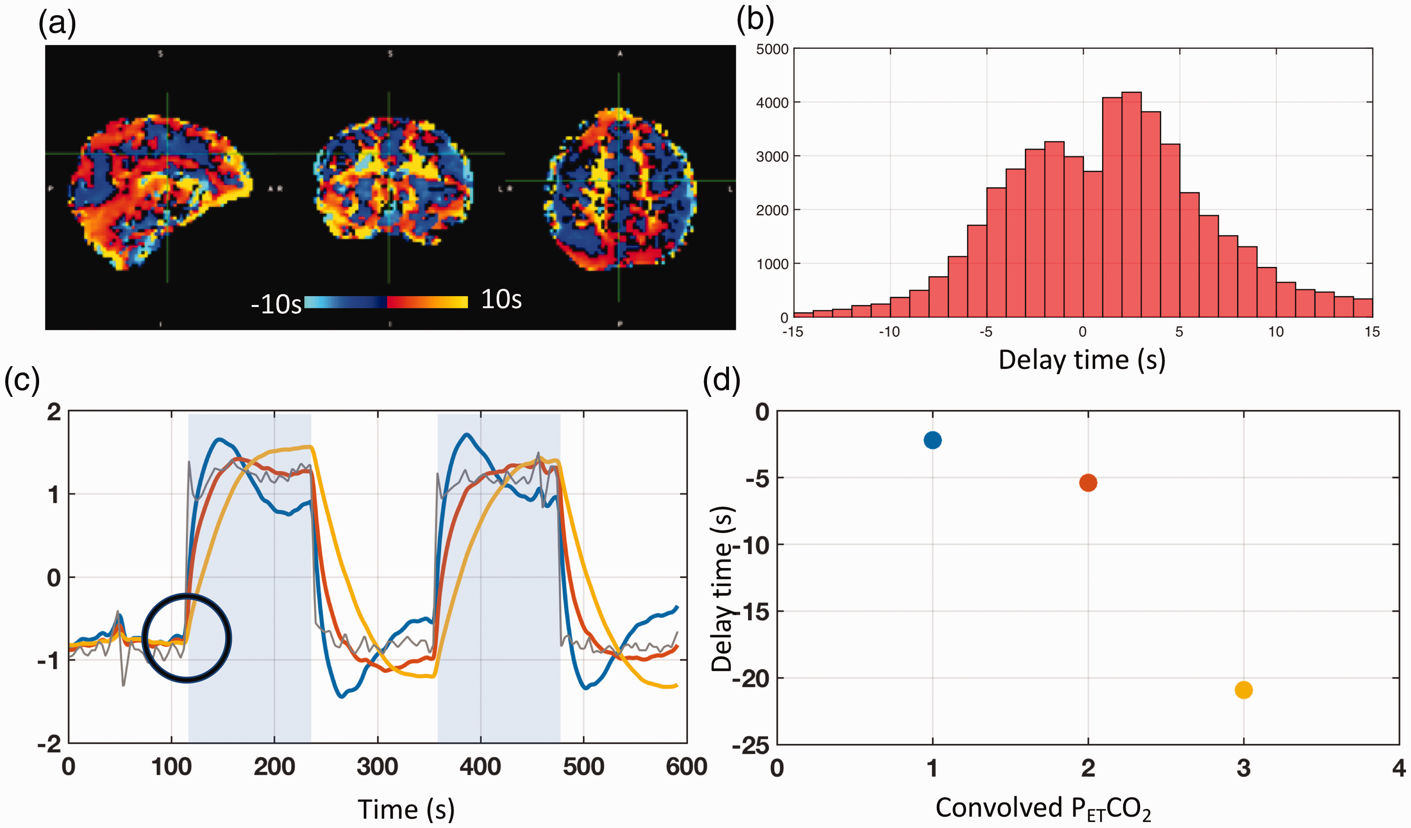
Real and simulated results of delay calculations using P_ETCO2-related-vLFO signal (∼0.004 Hz) from CO2 challenge data. (a) The delay map from a healthy subject undergoing a CO2 challenge. (b) The corresponding distribution of delay times for this subject, ranging from −15 s to 15 s. (c) The actual P_ETCO2 (in grey color) and three convolved P_ETCO2 signals (colors: blue, red, and yellow) are shown with a shared “break” point from baseline (black circle) in response to the elevated CO2. The delay times between the actual P_ETCO2 and the three convolved P_ETCO2 signals, ranging from −2 s to –21 s with significant maximum cross-correlation coefficient values (>0.9), are shown in (d) with their respective colors.

One possible explanation lies in a systematic error of cross-correlation method on P_ETCO2-related-vLFO signals (∼0.004 Hz). A simulation was conducted to illustrate this phenomenon. Three convolved P_ETCO2 time courses were generated (parameters of the three HRFs are: ( $α_{1}, β_{1}, β_{2}) = (1, 10, 10; 1, 10, 40; 1, 40, 40)$ ) to simulate a range of BOLD signal waveforms sharing the same “break” point from baseline (indicated by the black circle in Figure 7(c)). The three convolved P_ETCO2 time courses were cross-correlated with the actual P_ETCO2 to obtain time delays as done elsewhere.^23,24 Ideally, the delays should be close to zero given all the (synthesized) BOLD signals “reacted” to the elevated CO2 immediately; however, while highly significant MCCCs (>0.9) were obtained, the associated delays ranged from −2 s to −21 s (i.e., the P_ETCO2 was leading; see Figure 7(d))—distinctly not consistent with the constructed “immediate” response. This conflict indicates that the shape of the BOLD waveform can dramatically influence the outcome of a cross-correlation, leading to potentially-inaccurate delays. Therefore, we advocate that the sLFOs (CO2-demodulated) (which has much higher frequency)—rather than the P_ETCO2-related-vLFO—should be used to calculate the AT of the elevated CO2.

In addition, spurious correlation is always a big concern in the cross-correlation method.⁴⁵ Choosing a proper MCCC threshold is the most efficient way to obtain an accurate delay. From previous simulations using Monte Carlo or real fMRI signals (0.01∼0.1 Hz),^34,46 it was found that in order for LFO (0.01∼0.1 Hz) to have P < 0.01, the threshold of MCCC has to be adjusted to 0.3. We have also demonstrated quantitatively that the threshold (MCCC > 0.3) is sufficient in assessing the delay values in LFO, and P_ETCO2-related-vLFO signals (with less accuracy). However, the waveform effect (not random noise) is the dominant effect causing the extended delays in the CO2 studies. Lastly, other factors can also affect the delay calculation, such as high frequency components of the CO2 boxcar stimulus or motion artifacts left in the sLFO (CO2-demodulated) data. We conducted several simulations (supplemental materials Figure S7 and Figure S8) and found the limited impacts of these factors in this study.

Hemodynamic response function (HRF)

The second assumption of the traditional approach to calculate CVR values is that the entire brain responds to the CO2 challenge in a uniform manner. However, several studies show that the cerebral hemodynamic responses to hypercapnia are spatially-specific.^3,5,10,14 Given that the HRF in the CO2 challenge data reflecting the reaction of the blood vessel to the elevated CO2 may include its own delays, not excluding the arrival time of the CO2 from it could affect the accuracy of these HRFs.

In this study, we are able to separate the delay of the CO2 transport and the delay of the vasculature response. The former was addressed by obtaining the exact CO2 arrival time using the sLFO method. The latter was achieved by fitting a wide range of HRFs, after convolution with the shifted P_ETCO2, to BOLD signals. There are two advantages of using a limited number of HRF forms instead of performing multi-parameter voxel-specific fitting. First, it significantly shortens computing time (it would be easier to be adopted by other labs). Secondly, it avoids underdetermined fitting problems, making it easier to compare across subjects.

Consistent patterns were found in the HRF maps of the majority of the subjects, which demonstrate the spatial-specificity of the HRFs. Consistent with previous studies, this result supports the argument that different types of tissues and vessels will respond differently to elevated CO2. It is well known that arterial reaction to CO2 is immediate and fast,¹ while veins have no reaction to CO2. Moreover, different types of arteries⁴⁷ and even the same types of vessels with different diameters⁴⁸ were found to have different reactions to the CO2 challenge. Sato et al. found different CBF responses to elevated CO2 present in the internal carotid artery, external carotid artery, and vertebral artery due to a regional difference in CO2 regulation of blood flow among different cerebral circulatory areas.⁴⁷ Raper et al. found that the magnitude of the response to the elevated CO2 in the pial precapillary vessels has a higher increase in smaller vessels and lower increase in larger vessels.⁴⁸ These reactions, as partially reflected in the HRF maps, can be independent parameters to assess different brain conditions/diseases.

It is worth noting that some of the HRFs derived in this study as well as other similar studies⁵ are different from the typical HRF used in neurovascular coupling.^28,49 There are several possible explanations. First, underlying mechanisms of vascular response to CO2 and neurovascular response to neuronal firings are different in time, scale, and process. Secondly, the CO2 level increased sharply in the hypercapnia stage in this study, which is not the case in the neurovascular response or other processes (e.g., general respiration, breath-holding). Lastly, fast arterial reaction to the sharply increased CO2 might not be fully captured by the fMRI due to the low temporal resolution (i.e., TR), which limits the accuracy of HRFs. It would be of great interest to further explore these different mechanisms.

Cerebrovascular reactivity (CVR)

Our mean GM CVR and mean WM CVR values are in-line with previous studies.^12,50 The convolution of an accurate HRF and a shifted P_ETCO2 waveform allows us to better model the corresponding BOLD. In our proposed method, the R² values increased in the majority of the voxels across subjects, and some dramatically increased (4% ± 1% voxels have the increased R² values that are greater than the two standard deviations above the mean values). Consistent with prior literature,⁵ we have shown that having a spatial-specific HRF that models the BOLD signal accurately will improve the accuracy of CVR values. It is worth noting that an accurate AT alone does not improve a CVR value but help to derive an accurate local HRF. Both accurate parameters together can better model the BOLD for CO2 challenge.

Limitations and future studies

The primary limitations of this study are as follows. First, the HRF maps from subject 7 and 8 were different from those of subjects 1–6. One possible reason would be an error in estimation of the extra-cerebral delay (plausibly too short: 2–3 s), forcing (via equations 1–2) interpretation of longer within-brain delays. Such longer delays would result in best fits being achieved with our higher numbered HRFs, skewing the distribution relative to the other subjects. One possible solution could be the inclusion in the imaging volume of the internal carotid arteries. These would be ideal, as they represent the entry of the blood into the brain, and can be easily visually identified.^22,46 These two subjects also presented asymmetrical patterns in the HRF maps which were largely caused by the asymmetry of the original BOLD signals and the tilt of subjects’ heads during the scan (details can be found in the supplemental material Figure S9). Secondly, although 26 candidate HRFs were used to represent a wide range of cerebral hemodynamic responses, this set of HRFs is not likely to cover all situations, especially in aged or diseased populations. Additional ranges of parameters (which would, in turn, dictate additional reference HRFs) will be considered for future work. Thirdly, this study represents an evaluation of novel neurovascular measures only in healthy individuals. Future studies will apply this novel methodology to data from patients (e.g., victims of stroke or traumatic brain injury), as the mappings associated with AT, HRF and CVR can be expected to reflect different aspects of compromised vascular integrity. Note that among these parameters, AT (from RS-fMRI) and CVR have been examined individually in patients,^4–6,32,51 with abnormalities in diseased regions successfully detected. That said, the simultaneous application to patients of all three parameters remains to be addressed.

In conclusion, we successfully demonstrated a novel method that assesses multiple characteristics of the brain’s reaction to a CO2 challenge. In addition to CVR maps, the proposed method extracts two voxel-specific maps, reflecting further perfusion information. These maps represent rAT: the estimated CO2 arrival time at each brain region; and HRF: the hemodynamic response of how each brain region reacts to the elevated CO2. Lastly, we demonstrated the errors of rAT when using the P_ETCO2-related-vLFO signals (∼0.004 Hz) associated with the CO2 modulation.

Supplemental Material

sj-pdf-1-jcb-10.1177_0271678X20978582 - Supplemental material for A novel method of quantifying hemodynamic delays to improve hemodynamic response, and CVR estimates in CO2 challenge fMRI

Supplemental material, sj-pdf-1-jcb-10.1177_0271678X20978582 for A novel method of quantifying hemodynamic delays to improve hemodynamic response, and CVR estimates in CO2 challenge fMRI by Jinxia (Fiona) Yao, Ho-Ching (Shawn) Yang, James H Wang, Zhenhu Liang, Thomas M Talavage, Gregory G Tamer Jr Ikbeom Jang and Yunjie Tong in Journal of Cerebral Blood Flow & Metabolism

Footnotes

Acknowledgements

We thank two anonymous referees for their thoughtful suggestions that helped improve and clarify this manuscript significantly.

Funding

The author(s) disclosed receipt of the following financial support for the research, authorship, and/or publication of this article: This work was supported by the National Institutes of Health, Grants K25 DA031769 (YT); in part, with support from the Indiana Clinical and Translational Sciences Institute (the Pilot Funding for Research Use of Core Facilities).

Declaration of conflicting interests

The author (s) declared no potential conflicts of interest with respect to the research, authorship, and/or publication of this article.

Author’s contributions

The study was devised by YT. Experiments were performed by JFY, HSY, JHW, ZL and GGT. Data were analyzed by YT, JFY, HSY and IJ. Results were discussed, reviewed, interpreted, and compiled into final manuscript by YT, TMT, JFY, HSY, IJ, and GGT.

Supplemental material

Supplemental material for this paper can be found at

References

Reivich

Arterial pco2 and cerebral hemodynamics. Am J Physiol 1964; 206: 25–35.

Fierstra

Sobczyk

Battisti ‐ Charbonney

, et al. Measuring cerebrovascular reactivity: what stimulus to use? J Physiol 2013; 591: 5809–5821.

Duffin

Sobczyk

Crawley

, et al. The dynamics of cerebrovascular reactivity shown with transfer function analysis. Neuroimage 2015; 114: 207–216.

Geranmayeh

Wise

RJS

Leech

, et al. Measuring vascular reactivity with breath‐holds after stroke: a method to aid interpretation of group‐level BOLD signal changes in longitudinal fMRI studies. Hum Brain Mapp 2015; 36: 1755–1771.

Poublanc

Crawley

Sobczyk

, et al. Measuring cerebrovascular reactivity: the dynamic response to a step hypercapnic stimulus. J Cereb Blood Flow Metab 2015; 35: 1746–1756.

Chan

S-T

Evans

Rosen

, et al. A case study of magnetic resonance imaging of cerebrovascular reactivity: a powerful imaging marker for mild traumatic brain injury. Brain Inj 2015; 29: 403–407.

Svaldi

Joshi

Robinson

, et al. Cerebrovascular reactivity alterations in asymptomatic high school football players. Dev Neuropsychol 2015; 40: 80–84.

Liu

De Vis

Cerebrovascular reactivity (CVR) MRI with CO2 challenge: a technical review. NeuroImage 2019; 187: 104–115.

Ito

Mardimae

Han

, et al. Non‐invasive prospective targeting of arterial P CO 2 in subjects at rest. J Physiol 2008; 586: 3675–3682.

10.

Prokopiou

Pattinson

KTS

Wise

, et al. Modeling of dynamic cerebrovascular reactivity to spontaneous and externally induced CO2 fluctuations in the human brain using BOLD-fMRI. Neuroimage 2019; 186: 533–548.

11.

Bhogal

Siero

Fisher

, et al. Investigating the non-linearity of the BOLD cerebrovascular reactivity response to targeted hypo/hypercapnia at 7T. Neuroimage 2014; 98: 296–305.

12.

Bhogal

Philippens

Siero

, et al. Examining the regional and cerebral depth-dependent BOLD cerebrovascular reactivity response at 7T. Neuroimage 2015; 114: 239–248.

13.

Sobczyk

Battisti-Charbonney

Fierstra

, et al. A conceptual model for CO(2)-induced redistribution of cerebral blood flow with experimental confirmation using BOLD MRI. Neuroimage 2014; 92: 56–68.

14.

Golestani

Chang

Kwinta

, et al. Mapping the end-tidal CO2 response function in the resting-state BOLD fMRI signal: spatial specificity, test–retest reliability and effect of fMRI sampling rate. NeuroImage 2015; 104: 266–277.

15.

Blockley

Driver

Francis

, et al. An improved method for acquiring cerebrovascular reactivity maps. Magn Reson Med 2011; 65: 1278–1286.

16.

Thomas

Liu

Aslan

, et al. Physiologic underpinnings of negative BOLD cerebrovascular reactivity in brain ventricles. NeuroImage 2013; 83: 505–512.

17.

Donahue

Strother

Lindsey

, et al. Time delay processing of hypercapnic fMRI allows quantitative parameterization of cerebrovascular reactivity and blood flow delays. J Cereb Blood Flow Metab 2016; 36: 1767–1779.

18.

Tong

Lindsey

Hocke

, et al. Perfusion information extracted from resting state functional magnetic resonance imaging. J Cereb Blood Flow Metab 2017; 37: 564–576.

19.

Fisher

JA.

The CO2 stimulus for cerebrovascular reactivity: fixing inspired concentrations vs. targeting end-tidal partial pressures. J Cereb Blood Flow Metab 2016; 36: 1004–1011.

20.

Jenkinson

Beckmann

Behrens

, et al. Fsl. Neuroimage 2012; 62: 782–790.

21.

Power

Mitra

Laumann

, et al. Methods to detect, characterize, and remove motion artifact in resting state fMRI. Neuroimage 2014; 84: 320–341.

22.

Tong

Yao

Chen

, et al. The resting-state fMRI arterial signal predicts differential blood transit time through the brain. J Cereb Blood Flow Metab 2019; 39: 1148–1160.

23.

Thomas

Liu

Park

, et al. Cerebrovascular reactivity in the brain white matter: magnitude, temporal characteristics, and age effects. J Cereb Blood Flow Metab 2014; 34: 242–247.

24.

Yezhuvath

Lewis ‐ Amezcua

Varghese

, et al. On the assessment of cerebrovascular reactivity using hypercapnia BOLD MRI. NMR Biomed 2009; 22: 779–786.

25.

Gao

Liu

HL.

Inflow effects on functional MRI. Neuroimage 2012; 62: 1035–1039.

26.

Bradley

Jr Waluch

Lai

, et al. The appearance of rapidly flowing blood on magnetic resonance images. AJR Am J Roentgenol 1984; 143: 1167–1174.

27.

Shan

Wright

Thompson

, et al. Modeling of the hemodynamic responses in block design fMRI studies. J Cereb Blood Flow Metab 2014; 34: 316–324.

28.

Lindquist

Meng Loh

Atlas

, et al. Modeling the hemodynamic response function in fMRI: efficiency, bias and mis-modeling. Neuroimage 2009; 45: S187–S198.

29.

Wise

Ide

Poulin

, et al. Resting fluctuations in arterial carbon dioxide induce significant low frequency variations in BOLD signal. Neuroimage 2004; 21: 1652–1664.

30.

Birn

Smith

Jones

, et al. The respiration response function: the temporal dynamics of fMRI signal fluctuations related to changes in respiration. Neuroimage 2008; 40: 644–654.

31.

Hoffmann

2015. violin.m – Simple violin plot using Matlab default kernel density estimation. INRES (University of Bonn), Germany.

32.

Mandell

Han

Poublanc

, et al. Selective reduction of blood flow to white matter during hypercapnia corresponds with leukoaraiosis. Stroke 2008; 39: 1993–1998.

33.

Zhu

Xenos

Linninger

, et al. Dynamics of lateral ventricle and cerebrospinal fluid in normal and hydrocephalic brains. J Magn Reson Imaging 2006; 24: 756–770.

34.

Hocke

Tong

Lindsey

, et al. Comparison of peripheral near-infrared spectroscopy low-frequency oscillations to other denoising methods in resting state functional MRI with ultrahigh temporal resolution. Magn Reson Med 2016; 76: 1697–1707.

35.

Amemiya

Kunimatsu

Saito

, et al. Cerebral hemodynamic impairment: assessment with resting-state functional MR imaging. Radiology 2014; 270: 548–555.

36.

Christen

Jahanian

, et al. Noncontrast mapping of arterial delay and functional connectivity using resting-state functional MRI: a study in moyamoya patients. J Magn Reson Imaging 2015; 41: 424–430.

37.

Margulies

Cameron Craddock

, et al. Identifying the perfusion deficit in acute stroke with resting-state functional magnetic resonance imaging. Ann Neurol 2013; 73: 136–140.

38.

Ito

Kanno

Ibaraki

, et al. Changes in human cerebral blood flow and cerebral blood volume during hypercapnia and hypocapnia measured by positron emission tomography. J Cereb Blood Flow Metab 2003; 23: 665–670.

39.

Donahue

Faraco

Strother

, et al. Bolus arrival time and cerebral blood flow responses to hypercarbia. J Cereb Blood Flow Metab 2014; 34: 1243–1252.

40.

Y-CL

Petersen

Zimine

, et al. Similarities and differences in arterial responses to hypercapnia and visual stimulation. J Cereb Blood Flow Metab 2011; 31: 560–571.

41.

Mao

Liu

, et al. Multiparametric estimation of brain hemodynamics with MR fingerprinting ASL. Magn Reson Med 2017; 78: 1812–1823.

42.

Bumstead

Bauer

Wright

, et al. Cerebral functional connectivity and Mayer waves in mice: phenomena and separability. J Cereb Blood Flow Metab 2017; 37: 471–484.

43.

Rayshubskiy

Wojtasiewicz

Mikell

, et al. Direct, intraoperative observation of ∼ 0.1 Hz hemodynamic oscillations in awake human cortex: implications for fMRI. NeuroImage 2014; 87: 323–331.

44.

Champagne

Bhogal

Coverdale

, et al. A novel perspective to calibrate temporal delays in cerebrovascular reactivity using hypercapnic and hyperoxic respiratory challenges. Neuroimage 2019; 187: 154–165.

45.

Bright

Tench

Murphy

Potential pitfalls when denoising resting state fMRI data using nuisance regression. Neuroimage 2017; 154: 159–168.

46.

Yao

Wang

Yang

H-CS

, et al. Cerebral circulation time derived from fMRI signals in large blood vessels. J Magn Reson Imaging 2019; 50: 1504–1513.

47.

Sato

Sadamoto

Hirasawa

, et al. Differential blood flow responses to CO2 in human internal and external carotid and vertebral arteries. J Physiol 2012; 590: 3277–3290.

48.

Raper

Kontos

Patterson

LJ.

Response of pial precapillary vessels to changes in arterial carbon dioxide tension. Circ Res 1971; 28: 518–523.

49.

Aguirre

Zarahn

D'esposito

, et al. The variability of human, BOLD hemodynamic responses. NeuroImage 1998; 8: 360–369.

50.

McKetton

Sobczyk

Duffin

, et al. The aging brain and cerebrovascular reactivity. NeuroImage 2018; 181: 132–141.

51.

Donahue

Ayad

Moore

, et al. Relationships between hypercarbic reactivity, cerebral blood flow, and arterial circulation times in patients with moyamoya disease. J Magn Reson Imaging 2013; 38: 1129–1139.

Supplementary Material

Please find the following supplemental material available below.

For Open Access articles published under a Creative Commons License, all supplemental material carries the same license as the article it is associated with.

For non-Open Access articles published, all supplemental material carries a non-exclusive license, and permission requests for re-use of supplemental material or any part of supplemental material shall be sent directly to the copyright owner as specified in the copyright notice associated with the article.

0.00 MB

1.32 MB

A novel method of quantifying hemodynamic delays to improve hemodynamic response,and CVR estimates in CO2 challenge fMRI

Abstract

Keywords

Introduction

Materials and methods

Data acquisition

Data processing

Relative arrival time (rAT) map

Alignment of PETCO2 measurement

Hemodynamic Response Function (HRF) map

Cerebrovascular reactivity (CVR) map

Simulation to assess delay accuracy

Results

Relative arrival time (rAT) maps

Hemodynamic response function (HRF) maps

Cerebrovascular reactivity (CVR) maps

Errors in the delay calculations

Discussions

CO2 arrival time

Possible errors in assessing CO2 arrival time

Hemodynamic response function (HRF)

Cerebrovascular reactivity (CVR)

Limitations and future studies

Supplemental Material

sj-pdf-1-jcb-10.1177_0271678X20978582 - Supplemental material for A novel method of quantifying hemodynamic delays to improve hemodynamic response, and CVR estimates in CO2 challenge fMRI

Footnotes

Acknowledgements

Funding

Declaration of conflicting interests

Author’s contributions

Supplemental material

References

Supplementary Material

Alignment of P_ETCO2 measurement